Article

A Basic Asymptotic Test for Value-at-Risk Subadditivity

Department of Statistics and Actuarial Science, School of Computing and Data Science, The University of Hong Kong, Hong Kong SAR, China
Risks 2024, 12(12), 199; https://doi.org/10.3390/risks12120199
Submission received: 15 October 2024 / Revised: 2 December 2024 / Accepted: 9 December 2024 / Published: 10 December 2024
(This article belongs to the Special Issue Applied Financial and Actuarial Risk Analytics)

Abstract

:
An asymptotic hypothesis test for value-at-risk subadditivity is introduced and studied. The test is derived based on an equivalent formulation of the value-at-risk subadditivity inequality in terms of the distribution of the underlying risks’ sum. Its size is considered mathematically, and its power and p-value are studied empirically for different dependence structures, strength of dependence, marginal distributions, sample sizes, number of risks and value-at-risk confidence levels.

1. Introduction

Among other risk measures, value at risk (VaR) is widely used for computing regulatory capital, managing financial risks or assessing environmental risks. At confidence level α ( 0 , 1 ) , the value at risk (VaR) of a random loss X F X is the α -quantile of F X , which is
VaR α ( X ) : = F X 1 ( α ) = inf { x R : F X ( x ) α } ;
see Embrechts and Hofert (2013) for details about quantile functions. On the one hand, VaR always exists, is easy to interpret, is law invariant, monotone, translation invariant, positive-homogeneous and elicitable. On the other hand, VaR is in general not subadditive, so it does not necessarily respect the economic notion of diversification and is thus not a coherent risk measure (see Artzner et al. (1999)). However, it is still a popular ingredient of a risk manager’s toolbox that is applied, for example, if coherent alternatives such expected shortfall do not exist. In this paper, we present a basic asymptotic hypothesis test to assess whether, for a given joint loss distribution, possibly specified only through a sample, VaR is subadditive and thus a coherent risk measure. In the context of VaR estimation, a simple test of VaR α violations can be found in (McNeil et al. 2015, sct. 9.3.1).
To this end, let X = ( X 1 , , X d ) F X denote a random vector of d losses, for example, losses of a portfolio of size d or losses in d business lines of a financial firm; negative values represent gains. We are thus interested in computing VaR α ( S ) = F S 1 ( α ) for the aggregate loss
S = j = 1 d X j F S
at a given high confidence level α ( 0 , 1 ) ; for example, in the context of the Basel II guidelines, α = 0.99 for market risk and α = 0.999 for credit and operational risk. VaR is subadditive if  
F S 1 ( α ) j = 1 d F X j 1 ( α ) .
A mathematical verification of this inequality is only available in specific cases. One example is if X is jointly elliptical (see (McNeil et al. 2015, Theorem 8.28)). However, if two margins are not of the same type, it is already typically unclear whether VaR is subadditive. Another example concerns comonotone risks, in which case (McNeil et al. 2015, Proposition 7.20) guarantees equality in (1), so VaR is additive. However, this is usually a too strong of an assumption to be useful in practice.
There are four scenarios known under which VaR is known to often be superadditive, where F S 1 ( α ) > j = 1 d F X j 1 ( α ) . By (McNeil et al. 2015, sct. 2.3.5), these scenarios are
For a given joint loss distribution F X , or realizations from it, it is therefore important for risk managers to determine whether VaR α is superadditive. Note that the largest VaR α for given margins has been considered in various publications, including Embrechts et al. (2013), Boudt et al. (2015), Hofert et al. (2017), or Hofert (2020).
To assess VaR α superadditivity, we present a basic asymptotic one-sided t-test in Section 2, and we investigate its power and p-value empirically in Section 3. Section 4 contains concluding remarks; Appendix A briefly addresses the construction of Wilson score confidence intervals for the underlying F S ( s ) .

2. Asymptotic Hypothesis Test

By (Embrechts and Hofert 2013, Proposition 1 (5)), the subadditivity condition (1) is equivalent to
F S j = 1 d F X j 1 ( α ) α ,
which forms the basis of our hypothesis test. Although the equivalence of (1) and (2) also holds in case at least one of the margins F X 1 , , F X d is discrete, we typically have strictly increasing and continuous margins F X 1 , , F X d in mind, which is also standard when modeling financial risks.
A common problem in practice is information asymmetry, which is the fact that comparably much is known about the individual loss distributions F X j , j = 1 , , d , but rather little about F S due to the unknown dependence between X 1 , , X d . In such situations, one often models the dependence structure with a copula (see Nelsen (2006), (McNeil et al. 2015, chp. 7) or Hofert et al. (2018)). Information asymmetry may be due to the fact that joint losses may not happen in a synchronized way or that, after aggregation (for example, to monthly joint losses), there are too few joint losses for a meaningful estimation of F S in its right tail. We therefore treat F X j , j = 1 , , d , and corresponding values F X j 1 ( α ) as known, so we also assume to know
s = j = 1 d F X j 1 ( α ) .
F S is then typically specified in terms of an assumed copula C and the known margins F X j , j = 1 , , d , via Sklar’s theorem (see Sklar (1959)).
Even if we knew C, F S is typically still unknown to us; if it was known, we could try to verify (2) directly. We are thus interested in statistically assessing whether the true underlying F S satisfies (2), that is, we are interested in testing
H 0 : F S ( s ) α ( VaR α subadditive ) vs H 1 : F S ( s ) < α ( VaR α superadditive ) .
To this end, we estimate F S nonparametrically by its empirical distribution function
F ^ S , n ( x ) = 1 n i = 1 n 1 { S i x } , x R ,
based on n independent observations X 1 , , X n F X of joint losses with known margins F X 1 , , F X d and thus known s in (3), as well as S i = j = 1 d X i , j , i = 1 , , n . The following result provides the details of the test of (4).
Proposition 1
(Size α ˜ test). For significance level α ˜ ( 0 , 1 ) and sufficiently large n N , the test with test statistic
T n , d = n F ^ S , n ( s ) α F ^ S , n ( s ) ( 1 F ^ S , n ( s ) )
and critical region { T n , d < z α ˜ } for z α ˜ = Φ 1 ( α ˜ ) is a size α ˜ test of (4).
Proof. 
The test’s power is
P ( T n , d < z α ˜ ) = P n F ^ S , n ( s ) α F ^ S , n ( s ) ( 1 F ^ S , n ( s ) ) < z α ˜ = P n F ^ S , n ( s ) F S ( s ) F ^ S , n ( s ) ( 1 F ^ S , n ( s ) ) < z α ˜ + n α F S ( s ) F ^ S , n ( s ) ( 1 F ^ S , n ( s ) ) P n F ^ S , n ( s ) F S ( s ) F ^ S , n ( s ) ( 1 F ^ S , n ( s ) ) < z α ˜ n Φ ( z α ˜ ) = Φ ( Φ 1 ( α ˜ ) ) = α ˜ ,
where the inequality holds under H 0 (with equality if F S ( s ) = α , i.e., under additivity) and where the convergence holds by Slutsky’s theorem (Resnick 2014, Theorem 8.6.1) and the central limit theorem. □

3. Simulation Studies

In this section, we analyze the power and p-values computed for the test of (4) described in Proposition 1 via a simulation. Under different dependence structures (homogeneous normal copulas, t 4 copulas, Clayton copulas and Gumbel copulas), strength of dependence (such that Kendall’s tau τ is in { 0.2 , 0.5 , 0.8 } ), homogeneous marginal distribution functions ( N ( 0 , 1 ) , t 4 , Par ( 2 ) with distribution function F ( x ) = 1 ( 1 + x ) 2 , x 0 ), sample sizes n (in { 1000 , 10,000 } ) and number of risks (dimensions d in { 4 , 20 , 100 } ), we first consider estimates of the power function at significance level α ˜ = 0.05 as functions of the VaR confidence level α , and then we consider estimated p-values as functions of α . Finally, we investigate to what extent numerical issues may appear. The contributed R packages copula (Hofert et al. 2020), simsalapar (Hofert and Maechler 2018) and crop (Hofert 2016) were used to implement all simulations.

3.1. Estimated Power Function

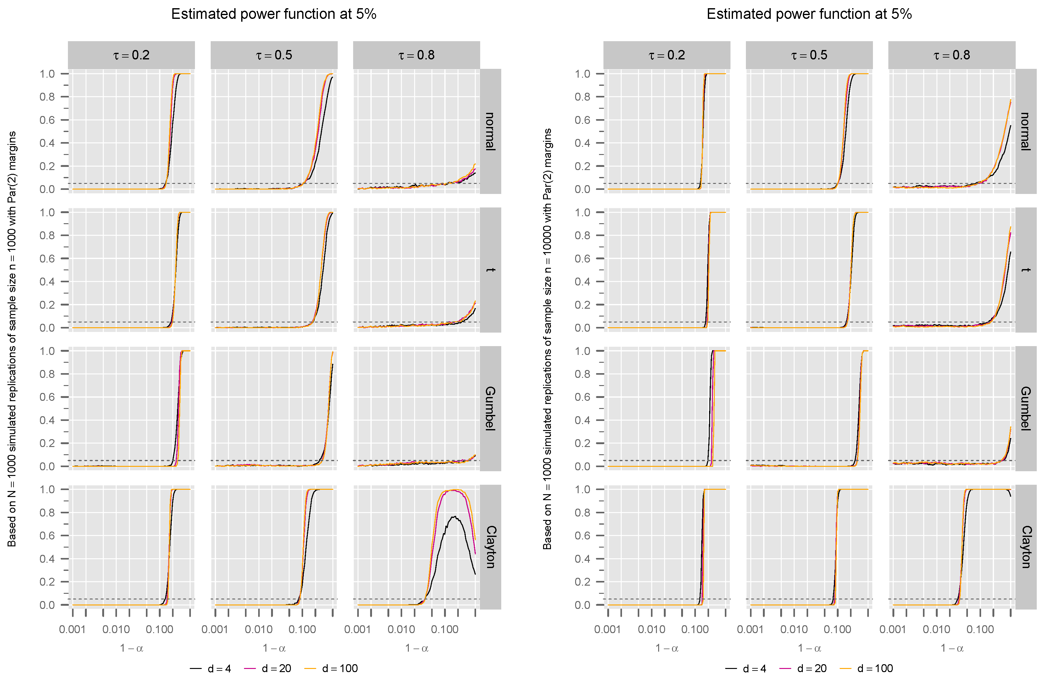
Figure 1 (for N ( 0 , 1 ) margins), Figure 2 (for t 4 margins) and Figure 3 (for Par ( 2 ) margins) show empirical estimates π ^ 0.05 of the power function π 0.05 at 5% (based on N = 1000 simulated replications of sample size n = 1000 each (left-hand side figure) and of sample size n = 10,000 each (right-hand side figure)) as a function of 1 α for the VaR confidence level α , for each of the considered copulas (in different rows) and strength of dependence in terms of Kendall’s tau (in different columns), and this occurs for d = 4 (black lines), d = 20 (red lines) and d = 100 (yellow lines) losses.
In the first row of Figure 1, the parameter choices are such that we have an underlying joint normal distribution; thus, we know, by (McNeil et al. 2015, Theorem 8.28 (2)), that VaR α is subadditive if and only if 1 α 1 / 2 , which is in line with our test’s estimated power function. Similarly, for the second row of Figure 2, where the parameter choices are such that we have an underlying joint t 4 distribution for which, also by (McNeil et al. 2015, Theorem 8.28 (2)), we know that VaR α is subadditive if and only if 1 α 1 / 2 . Under the setups of all other rows of plots in Figure 1, Figure 2 and Figure 3, it is unknown whether VaR α is subadditive.
Overall, we see that the estimated power π ^ 0.05 of the test is barely affected by the considered sample sizes n { 1000 , 10,000 } , strengths of dependence τ { 0.2 , 0.5 , 0.8 } and dimensions d { 4 , 20 , 100 } . It is mostly influenced by the type of dependence and margins.

3.2. Estimated p-Values by Simulation

Figure 4 (for N ( 0 , 1 ) margins), Figure 5 (for t 4 margins) and Figure 6 (for Par ( 2 ) margins) show empirical estimates of the p-values (based on N = 1000 simulated replications of sample size n = 1000 each (left-hand side figure) and of sample size n = 10,000 each (right-hand side figure)) as a function of 1 α for the VaR confidence level α for each of the considered copulas (in different rows) and strength of dependence in terms of Kendall’s tau (in different columns), and this occurs for d = 4 (black lines), d = 20 (red lines) and d = 100 (yellow lines) losses.
As in Section 3.1, we have an underlying joint normal distribution in the first row of Figure 4 and an underlying joint t 4 distribution in the second row of Figure 5. Moreover, we know that VaR α is subadditive if and only if 1 α 1 / 2 in each of these two cases, which is in line with our test’s estimated p-values. Comparing the last rows of Figure 4, Figure 5 and Figure 6, we observe that heavier-tailed margins paired with more strongly concordant Clayton copulas lead to smaller p-values for those α not too close to 1.
Overall, we again see that the estimated p-values of the test are affected rather little by the considered sample sizes n { 1000 , 10,000 } , strengths of dependence τ { 0.2 , 0.5 , 0.8 } and dimensions d { 4 , 20 , 100 } , and that they are mostly rather depend on the type of dependence and margins.

3.3. A Numerical Issue

Although not visible from the estimated power functions and p-values, but anticipated from the form of the test statistic T n , d in Proposition 1, the test may be unreliable if F ^ S , n ( s ) is close to 0 or 1. In these cases, T n , d can explode to under H 0 , leading to no rejection of H 0 , and T n , d can explode to under H 1 , leading to rejection of H 0 . Although these two decisions are correct in these two scenarios, the test may become unreliable; therefore, one should check how severe this problem is.
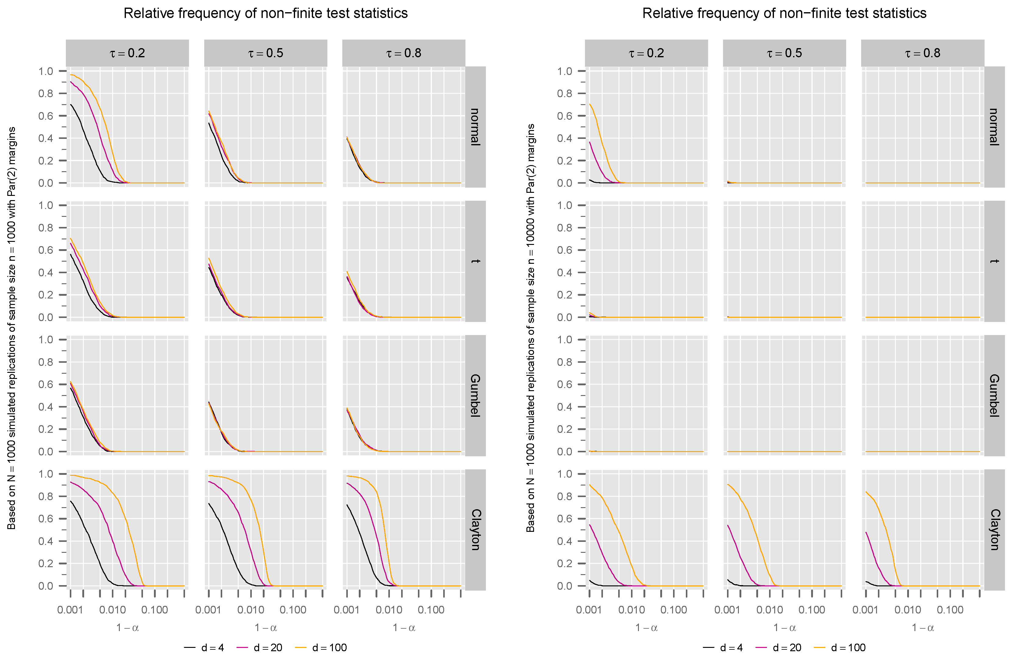
Under the same setups as considered in Section 3.1 and Section 3.2, Figure 7 (for N ( 0 , 1 ) margins), Figure 8 (for t 4 margins) and Figure 9 (for Par ( 2 ) margins) show the relative frequency of non-finite test statistics T n , d (based on N = 1000 simulated replications of sample size n = 1000 each (left-hand side figure) and of sample size n = 10,000 each (right-hand side figure)) as a function of 1 α for the VaR confidence level α , for each of the considered copulas (in different rows) and strength of dependence in terms of Kendall’s tau (in different columns), and this occurs for d = 4 (black lines), d = 20 (red lines) and d = 100 (yellow lines) losses.
Unsurprisingly, the problem is more present for a large α (a known statistical challenge when estimating VaR α and other tail-based risk measures) and less present for a larger sample size n (compare, for example, the two third rows in Figure 7). More interestingly, weaker dependencies ( τ = 0.2 ) tend to lead to more non-finite test statistics than stronger dependencies (see, for example, the left-hand side plots in Figure 7). Although one would typically rather consider radially symmetric dependence models or models with upper tail dependence rather than just lower tail dependence, the Clayton case is worth mentioning as being particularly challenging when it comes to the problem of non-finite realized test statistics. The problem does not seem to vanish much for a larger n and becomes more severe for a larger dimension d (unlike the other cases considered), and this occurs across all considered margins.

4. Conclusions

When working with VaR α as a risk measure in quantitative risk management practice, a central question is whether VaR α is subadditive for the particular joint distribution under consideration. To this end, we presented a basic and straightforward method to compute an asymptotic hypothesis test, showing that it is a size α ˜ test (for α ˜ being the significance level) and studied it numerically (as a function of 1 α ) for various dependence models, strength of dependence, marginal distributions, dimensions and sample sizes. The test performed well overall, but requires a sufficiently large sample size n and not too large of a confidence level α to lead to reliable results when based on actual (rather than simulated) data. Due to its dependence on the empirical distribution of the sum, one particular challenge when applied to actual data is that of an exploding test statistic, which we identified as especially challenging in the case of Clayton dependence structures. Clearly, when based on actual data, hypothesis tests should only be viewed as providing one additional tool for assessing VaR α sub- vs. superadditivity, rather than basing such a decision solely on the result of a single statistical test. Nevertheless, if tests can raise suspicion about the model used, they can ultimately lead to improved models and thus contribute to the stability of the financial system as a whole.
Three of the four known scenarios mentioned in Section 1, under which VaR α is known to often be superadditive, assume the dependence structure to be the independence copula. Under dependence, besides the rather extreme special case of a countermonotone joint tail, not much is known. As our test results hint at, under more realistic dependencies, VaR α does not typically seem to be superadditive. Future work could specifically investigate this for more joint models.
Another avenue for future research is to treat the margins as unknown and thus to estimate them. The test’s p-value could then be bootstrapped, and the correctness of the whole procedure would need to be studied via a simulation.

Funding

This research received no external funding.

Data Availability Statement

No new data were created or analyzed in this study. Data sharing is not applicable to this article.

Conflicts of Interest

The author declares no conflicts of interest.

Appendix A. Asymptotic Confidence Interval for FS(s)

This appendix addresses how asymptotic confidence intervals (CIs) can be constructed for F S ( s ) . We already utilized asymptotic normality of F ^ S , n ( s ) in the proof of Proposition 1. By Slutsky’s theorem,
n F ^ S , n ( s ) F S ( s ) F ^ S , n ( s ) ( 1 F ^ S , n ( s ) ) n N ( 0 , 1 ) ,
from which the straightforward Wald ( 1 α ˜ ) -CI
F ^ S , n ( s ) F ^ S , n ( s ) ( 1 F ^ S , n ( s ) ) n z 1 α ˜ / 2 , F ^ S , n ( s ) + F ^ S , n ( s ) ( 1 F ^ S , n ( s ) ) n z 1 α ˜ / 2
for F S ( s ) results. To avoid the zero-width and overshooting problems of Wald CIs, we construct a Wilson score interval (see Newcombe (1998) and Wilson (1927), respectively).
To obtain the endpoints of a Wilson score interval, one starts from the asymptotic normality of n F ^ S , n ( s ) F S ( s ) F S ( s ) ( 1 F S ( s ) ) and solves n F ^ S , n ( s ) F S ( s ) F S ( s ) ( 1 F S ( s ) ) = ± z 1 α ˜ / 2 . This is equivalent to solving n | F ^ S , n ( s ) F S ( s ) | F S ( s ) ( 1 F S ( s ) ) = z 1 α ˜ / 2 , so ( F ^ S , n ( s ) F S ( s ) ) 2 = z 1 α ˜ / 2 2 n F S ( s ) ( 1 F S ( s ) ) ; thus, 1 + z 1 α ˜ / 2 2 n F S ( s ) 2 2 F ^ S , n ( s ) + z 1 α ˜ / 2 2 n F S ( s ) + F ^ S , n ( s ) 2 = 0 . Solving this quadratic equation in F S ( s ) leads to the endpoints
2 F ^ S , n ( s ) + z 1 α ˜ / 2 2 n ± 2 F ^ S , n ( s ) + z 1 α ˜ / 2 2 n 2 4 1 + z 1 α ˜ / 2 2 n F ^ S , n ( s ) 2 2 1 + z 1 α ˜ / 2 2 n
of the ( 1 α ˜ ) -CI (Wilson score interval), which simplifies to
I n , α ˜ / 2 , ± : = F ^ S , n ( s ) + z 1 α ˜ / 2 2 2 n ± z 1 α ˜ / 2 F ^ S , n ( s ) ( 1 F ^ S , n ( s ) ) n + z 1 α ˜ / 2 2 4 n 2 1 + z 1 α ˜ / 2 2 n .
Due to the nature of our problem of determining VaR sub- or superadditivity, we can utilize a respective one-sided ( 1 α ˜ ) -CI for F S ( s ) : If α [ I n , α ˜ , , 1 ] (that is, α < I n , α ˜ , ) then VaR α is subadditive (that is, F S ( s ) α ) with confidence at least 1 α ˜ .
Finally, note that a one-sided simultaneous ( 1 α ˜ ) -CIs for F S can be constructed with the one-sided Dvoretzky–Kiefer–Wolfowitz inequality (see, for example, Massart (1990)), according to which, for all ε log ( 2 ) / ( 2 n ) ,
P ( F S ( s ) [ F ^ S , n ( s ) ε , 1 ] s ) = P ( F ^ S , n ( s ) F S ( s ) ε s ) = P ( sup s R ( F ^ S , n ( s ) F ( s ) ) ε ) = 1 P ( sup s R ( F ^ S , n ( s ) F ( s ) ) > ε ) 1 e 2 n ε 2 ,
which equals 1 α ˜ if and only if ε = log ( α ˜ ) / ( 2 n ) and which is valid for all α ˜ [ 0 , 1 / 2 ] . The corresponding simultaneous one-sided ( 1 α ˜ ) -CI for F S is therefore
I n , α ˜ ( s ) = F ^ S , n ( s ) log ( α ˜ ) 2 n , 1 , s R .
We can now argue similarly as for the pointwise asymptotic Wilson score interval before: if α I n , α ˜ ( s ) (that is, α < F ^ S , n ( s ) log ( α ˜ ) / ( 2 n ) ), then VaR α is subadditive with confidence at least 1 α ˜ .

References

  1. Artzner, Philippe, Freddy Delbaen, Jean-Marc Eber, and David Heath. 1999. Coherent measures of risk. Mathematical Finance 9: 203–28. [Google Scholar] [CrossRef]
  2. Boudt, Kris, Edgars Jakobsons, and Steven Vanduffel. 2015. Block rearranging elements within matrix columns to minimize the variability of the row sums. 4OR-A Quarterly Journal of Operations Research 16: 31–50. [Google Scholar] [CrossRef]
  3. Embrechts, Paul, Alexander J. McNeil, and Daniel Straumann. 2002. Correlation and dependency in risk management: Properties and pitfalls. In Risk Management: Value at Risk and Beyond. Edited by Michael Dempster. Cambridge, MA: Cambridge University Press, pp. 176–223. [Google Scholar]
  4. Embrechts, Paul, and Marius Hofert. 2013. A note on generalized inverses. Mathematical Methods of Operations Research 77: 423–32. [Google Scholar] [CrossRef]
  5. Embrechts, Paul, Andrea Höing, and Giovanni Puccetti. 2005. Worst var scenarios. Insurance: Mathematics and Economics 37: 115–34. [Google Scholar] [CrossRef]
  6. Embrechts, Paul, Giovanni Puccetti, and Ludger Rüschendorf. 2013. Model uncertainty and var aggregation. Journal of Banking & Finance 37: 2750–64. [Google Scholar]
  7. Hofert, Marius. 2016. Crop: Graphics Cropping Tool. R Package Version 0.0-3. Madison: R Package Vignette. [Google Scholar] [CrossRef]
  8. Hofert, Marius. 2020. Implementing the Rearrangement Algorithm: An Example from Computational Risk Management. Risks 8: 47. [Google Scholar] [CrossRef]
  9. Hofert, Marius, Amir Memartoluie, David Saunders, and Tony Wirjanto. 2017. Improved algorithms for computing worst Value-at-Risk. Statistics & Risk Modeling 34: 13–31. [Google Scholar] [CrossRef]
  10. Hofert, Marius, and Alexander J. McNeil. 2015. Subadditivity of value-at-risk for bernoulli random variables. Statistics & Probability Letters 98: 79–88. [Google Scholar] [CrossRef]
  11. Hofert, Marius, and Martin Maechler. 2018. simsalapar: Tools for Simulation Studies in Parallel with R. R Package Version 1.0-10. Madison: R Package Vignette. [Google Scholar] [CrossRef]
  12. Hofert, Marius, Ivan Kojadinovic, Martin Maechler, Jun Yan, Johanna G. Nešlehová, and Rebecca Morger. 2020. copula: Multivariate Dependence with Copulas. R Package Version 1.0.0. Madison: R Package Vignette. [Google Scholar] [CrossRef]
  13. Hofert, Marius, Ivan Kojadinovic, Martin Mächler, and Jun Yan. 2018. Elements of Copula Modeling with R. Springer Use R! Series; Cham: Springer. [Google Scholar] [CrossRef]
  14. Massart, Pascal. 1990. The tight constant in the Dvoretzky–Kiefer–Wolfowitz inequality. The Annals of Probability 18: 1269–83. [Google Scholar] [CrossRef]
  15. McNeil, Alexander J., Rüdiger Frey, and Paul Embrechts. 2015. Quantitative Risk Management: Concepts, Techniques and Tools, 2nd ed. Princeton: Princeton University Press. [Google Scholar]
  16. Nelsen, Roger B. 2006. An Introduction to Copulas. New York: Springer. [Google Scholar]
  17. Newcombe, Robert G. 1998. Two-sided confidence intervals for the single proportion: Comparison of seven methods. Statistics in Medicine 17: 857–72. [Google Scholar] [CrossRef]
  18. Resnick, Sidney I. 2014. A Probability Path. Basel: Birkhäuser. [Google Scholar]
  19. Sklar, Abe. 1959. Fonctions de répartition à n dimensions et leurs marges. Publications de L’Institut de Statistique de L’Université de Paris 8: 229–31. [Google Scholar]
  20. Wilson, Edwin B. 1927. Probable inference, the law of succession, and statistical inference. Journal of the American Statistical Association 22: 209–12. [Google Scholar] [CrossRef]
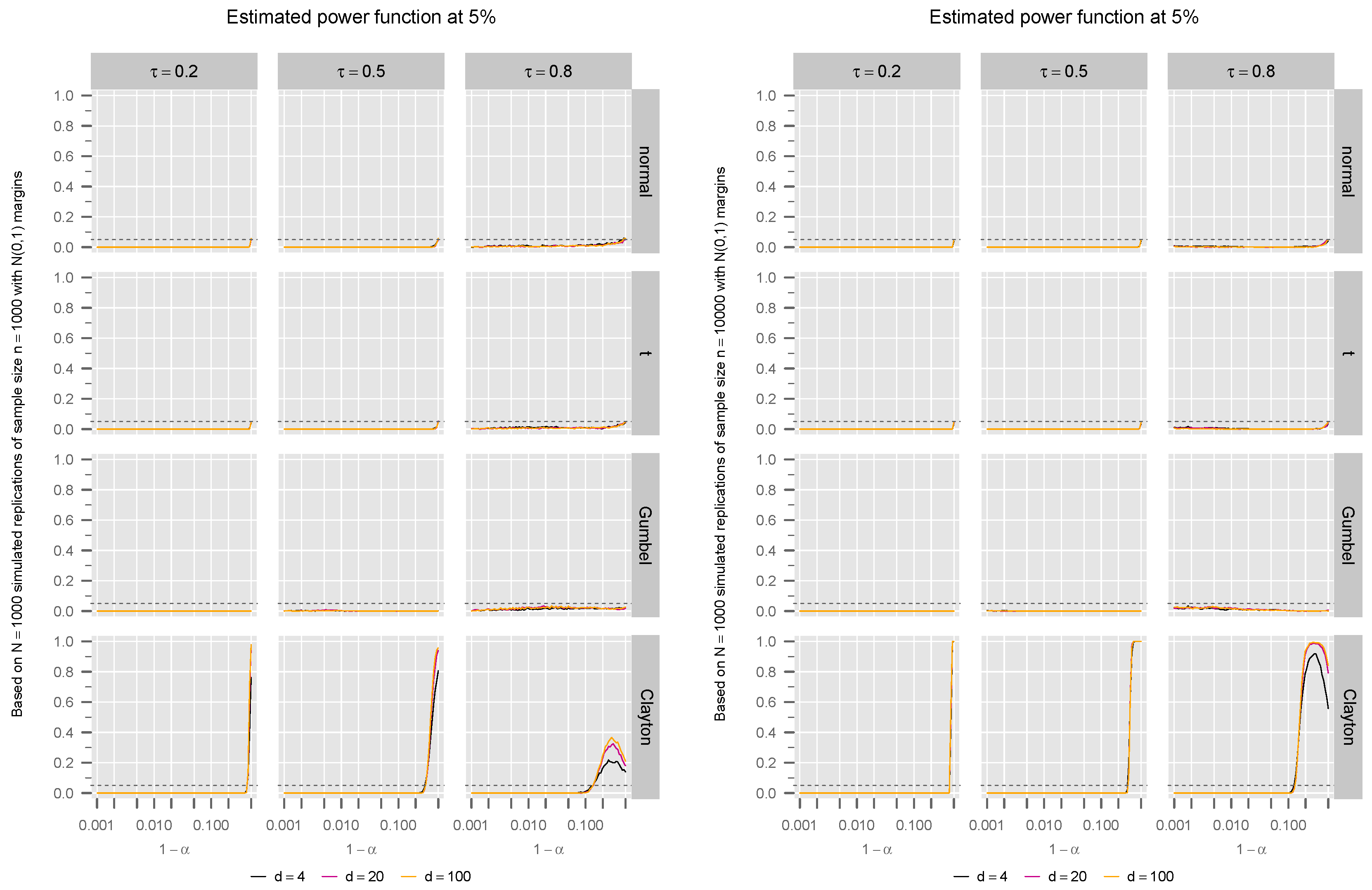
Figure 1. Estimated power π ^ 0.05 (5% indicated by a dashed line) as a function of 1 α for VaR confidence level α [ 0.5 , 0.999 ] in dimensions d { 4 , 20 , 100 } (solid lines) under normal, t 4 , Clayton and Gumbel copulas with (homogeneous) parameters such that τ { 0.2 , 0.5 , 0.8 } and with N ( 0 , 1 ) margins, where each curve is an average over N = 1000 simulated replications of samples of size n = 1000 (left) or n = 10,000 (right). For the cases in the first row (joint normal distribution), we know analytically that VaR is subadditive for all displayed 1 α .
Risks 12 00199 g001
Figure 2. Estimated power π ^ 0.05 (5% indicated by a dashed line) as a function of 1 α for VaR confidence level α [ 0.5 , 0.999 ] in dimensions d { 4 , 20 , 100 } (solid lines) under normal, t 4 , Clayton and Gumbel copulas with (homogeneous) parameters such that τ { 0.2 , 0.5 , 0.8 } and with t 4 margins, where each curve is an average over N = 1000 simulated replications of samples of size n = 1000 (left) or n = 10,000 (right). For the cases in the second row (joint t 4 distribution), we know analytically that VaR is subadditive for all displayed 1 α .
Risks 12 00199 g002
Figure 3. Estimated power π ^ 0.05 (5% indicated by a dashed line) as a function of 1 α for VaR confidence level α [ 0.5 , 0.999 ] in dimensions d { 4 , 20 , 100 } (solid lines) under normal, t 4 , Clayton and Gumbel copulas with (homogeneous) parameters such that τ { 0.2 , 0.5 , 0.8 } and with Par ( 2 ) margins, where each curve is an average over N = 1000 simulated replications of samples of size n = 1000 (left) or n = 10,000 (right). For none of the displayed cases do we know analytically whether VaR is subadditive for all displayed 1 α .
Risks 12 00199 g003
Figure 4. Estimated p-values (identity and thus significance level) indicated by a dashed line) as a function of 1 α for VaR confidence level α [ 0.5 , 0.999 ] in dimensions d { 4 , 20 , 100 } (solid lines) under normal, t 4 , Clayton and Gumbel copulas with (homogeneous) parameters such that τ { 0.2 , 0.5 , 0.8 } and with N ( 0 , 1 ) margins, where each curve is an average over N = 1000 simulated replications of samples of size n = 1000 (left) or n = 10,000 (right). For the cases in the first row (joint normal distribution), we know analytically that VaR is subadditive for such α .
Risks 12 00199 g004
Figure 5. Estimated p-values (identity and thus significance level) as a function of 1 α for VaR confidence level α [ 0.5 , 0.999 ] in dimensions d { 4 , 20 , 100 } (solid lines) under normal, t 4 , Clayton and Gumbel copulas with (homogeneous) parameters such that τ { 0.2 , 0.5 , 0.8 } and with t 4 margins, where each curve is an average over N = 1000 simulated replications of samples of size n = 1000 (left) or n = 10,000 (right). For the cases in the second row (joint t 4 distribution), we know analytically that VaR is subadditive for such α .
Risks 12 00199 g005
Figure 6. Estimated p-values (identity and thus significance level) as a function of 1 α for VaR confidence level α [ 0.5 , 0.999 ] in dimensions d { 4 , 20 , 100 } (solid lines) under normal, t 4 , Clayton and Gumbel copulas with (homogeneous) parameters such that τ { 0.2 , 0.5 , 0.8 } and with Par ( 2 ) margins, where each curve is an average over N = 1000 simulated replications of samples of size n = 1000 (left) or n = 10,000 (right). For none of the displayed cases do we know analytically whether VaR is subadditive for such α .
Risks 12 00199 g006
Figure 7. Relative frequency of non-finite test statistics as a function of 1 α for VaR confidence level α [ 0.5 , 0.999 ] in dimensions d { 4 , 20 , 100 } (solid lines) under normal, t 4 , Clayton and Gumbel copulas with (homogeneous) parameters such that τ { 0.2 , 0.5 , 0.8 } and with N ( 0 , 1 ) margins, where each curve is an average over N = 1000 simulated replications of samples of size n = 1000 (left) or n = 10,000 (right).
Risks 12 00199 g007
Figure 8. Relative frequency of non-finite test statistics as a function of 1 α for VaR confidence level α [ 0.5 , 0.999 ] in dimensions d { 4 , 20 , 100 } (solid lines) under normal, t 4 , Clayton and Gumbel copulas with (homogeneous) parameters such that τ { 0.2 , 0.5 , 0.8 } and with t 4 margins, where each curve is an average over N = 1000 simulated replications of samples of size n = 1000 (left) or n = 10,000 (right).
Risks 12 00199 g008
Figure 9. Relative frequency of non-finite test statistics as a function of 1 α for VaR confidence level α [ 0.5 , 0.999 ] in dimensions d { 4 , 20 , 100 } (solid lines) under normal, t 4 , Clayton and Gumbel copulas with (homogeneous) parameters such that τ { 0.2 , 0.5 , 0.8 } and with Par ( 2 ) margins, where each curve is an average over N = 1000 simulated replications of samples of size n = 1000 (left) or n = 10,000 (right).
Risks 12 00199 g009
Disclaimer/Publisher’s Note: The statements, opinions and data contained in all publications are solely those of the individual author(s) and contributor(s) and not of MDPI and/or the editor(s). MDPI and/or the editor(s) disclaim responsibility for any injury to people or property resulting from any ideas, methods, instructions or products referred to in the content.