Enhancing Portfolio Decarbonization Through SensitivityVaR and Distorted Stochastic Dominance

Abstract

Recent trends in portfolio management emphasize the importance of reducing carbon footprints and aligning investments with sustainable practices. This paper introduces Sensitivity Value-at-Risk (SensitivityVaR), an advanced distortion risk measure that combines Value-at-Risk (VaR) and Expected Shortfall (ES) with the Cornish–Fisher expansion. SensitivityVaR provides a more robust framework for managing risk, particularly under extreme market conditions. By incorporating first- and second-order distorted stochastic dominance criteria, we enhance portfolio decarbonization strategies, aligning financial objectives with environmental targets such as the Paris Agreement’s goal of a 7% annual reduction in carbon intensity from 2019 to 2050. Our empirical analysis evaluates the impact of integrating carbon intensity data—including Scope 1, Scope 2, and Scope 3 emissions—on portfolio optimization, focusing on key sectors like technology, energy, and consumer goods. The results demonstrate the effectiveness of SensitivityVaR in managing both risk and environmental impact. The methodology led to significant reductions in carbon intensity across different portfolio configurations, while preserving competitive risk-adjusted returns. By optimizing tail risks and limiting exposure to carbon-intensive assets, this approach produced more balanced and efficient portfolios that aligned with both financial and sustainability goals. These findings offer valuable insights for institutional investors and asset managers aiming to integrate climate considerations into their investment strategies without compromising financial performance.

1. Introduction

In the domain of decision-making under conditions of uncertainty, individuals assign different levels of significance to uncertain outcomes based on their personal preferences. These differences often lead to subjective biases or misjudgments. The process of prioritizing these uncertainties involves the transformation of values associated with random variables or their distribution functions. Techniques such as integrated distribution functions, utility theory, and probability distortions become vital. Exploring the theory of stochastic dominance reveals a set of tools designed to express preferences and risk attitudes, influenced by these transformations. Commonly used in economics, finance, and insurance, stochastic dominance is essential for understanding and managing decision-making under uncertainty.

In portfolio management, two predominant approaches guide the selection process: the mean-risk criterion and the stochastic dominance criterion. The mean-risk criterion involves maximizing expected returns while minimizing risk, with the risk level being determined by the investor’s risk tolerance. However, this approach does not account for all types of investor risk behavior (Ogryczak and Ruszczyński 2001). In some cases, it may lead to optimal solutions that do not meet the stochastic dominance criterion. The stochastic dominance criterion ranks random variables by using their distribution functions and is consistent with utility theory. Two prevalent types of stochastic dominance relations—first-order stochastic dominance (FSD) and second-order stochastic dominance (SSD)—are commonly utilized. FSD is favored by decision-makers who prefer “more” to “less”, whereas SSD appeals to those who are risk-averse, offering a nuanced reflection of a decision-maker’s attitude towards risk and preferences. However, it is generally quite challenging to determine whether one uncertain prospect is better than another. As a result, the discriminative power of FSD is often poor. On the other hand, SSD may be limiting for decision-makers who are mainly risk-averse but may have some degree of flexibility in their preferences and exhibit a weak risk attitude. This has been discussed in detail by Leshno and Levy (2002) and more recently by Müller et al. (2017).

The primary goal of portfolio management is to optimize the balance between risk and return, and risk measures has essential role in this process. conventional risk measures such as Value-at-Risk (VaR) and Expected Shortfall (ES) are widely used in financial risk management but have well-documented limitations. VaR does not provide information about the severity of losses beyond its threshold and is not sub-additive, potentially underestimating risk (Artzner et al. 1999b). ES, while addressing some of VaR’s shortcomings by considering the tail-end of the loss distribution, can be computationally intensive and sensitive to extreme values (Acerbi and Tasche 2002). These limitations necessitate more flexible approaches that account for extreme market conditions and tail risks, including the use of distortion risk measures (DRMs) and quantile-based techniques.

Several advanced risk measures have been proposed to address these limitations. For example, the use of quantile-based and expectile-based measures has gained traction in risk management (Bellini et al. 2014). These approaches better capture tail risk and provide more robust risk assessment under extreme market conditions. Additionally, the linear combination of VaR and ES has been explored to optimize risk management under specific constraints, as demonstrated by Xiong et al. (2023). In this context, DRMs, such as GlueVaR introduced by Belles-Sampera et al. (2014), provide flexibility in modeling risk attitudes and tail behavior. Recent studies have further emphasized the integration of distortion risk measures into portfolio management strategies. For instance, Trabelsi and Tiwari (2019) explore market risk optimization using CVaR measures and copulas, which align closely with the need for distortion risk measures in multi-risk settings. Zhu and Li (2012) contribute to this discussion by analyzing tail distortion risk measures, emphasizing their ability to manage downside risk more effectively than conventional methods.

Several studies have explored advanced risk measures and their applications in portfolio management, emphasizing the importance of integrating robust risk measures to address market complexities. For instance, Syuhada et al. (2023) introduces expected-based VaR and ES using quantile and expectile, which align with the concept of distorted stochastic dominance. Additionally, Kabaila and Syuhada (2010) discuss the asymptotic efficiency of improved prediction intervals, providing foundational insights relevant to our use of the Cornish–Fisher expansion. Furthermore, recent studies such as the one conducted by Minasyan (2021) develop new classes of distortion risk measures, showcasing their flexibility and robustness in various financial applications. These works, along with other studies on advanced risk measures Belles-Sampera et al. (2014); Rockafellar et al. (2000), provide a solid base of literature and context for the current study, underscoring the relevance and novelty of our approach.

SensitivityVaR leverages distorted stochastic dominance principles, providing better alignment between financial risk management and sustainability objectives. This paper introduces SensitivityVaR, a risk measure that combines VaR and ES using the Cornish–Fisher expansion, which accounts for skewness and kurtosis in return distributions (Cornish and Fisher 1938; Fisher and Cornish 1960). This approach enhances the accuracy of risk measures in asset return distributions (Amédée-Manesme et al. 2019), and has been applied to distortion risk measures like GlueVaR (Belles-Sampera et al. 2016). Although SensitivityVaR focuses on financial risk, it is employed within a portfolio optimization framework that integrates carbon intensity constraints. By incorporating first- and second-order distorted stochastic dominance, this approach allows for the alignment of risk management with sustainability goals, ensuring that portfolios meet both financial performance and environmental impact targets.

The integration of SensitivityVaR in portfolio decarbonization aligns with existing research emphasizing sustainable investment practices.This study builds upon the work of Salo et al. (2023) and Steuer and Utz (2023) by offering a concrete methodology for portfolio decarbonization that not only optimizes financial performance but also directly integrates carbon intensity metrics into the risk framework. The primary contribution of this paper is the development of SensitivityVaR that merges conventional risk measures with carbon intensity considerations, offering investors a more comprehensive framework for sustainable portfolio management. This paper contributes to the literature by integrating financial risk with environmental sustainability, with implications for both theoretical development and practical portfolio strategies.

This paper is structured as follows. Section 2 discusses innovating risk measures: SensitivityVaR formulation and validation, detailing the Cornish–Fisher expansion and presenting theoretical insights and preliminary simulations. Section 3 elaborates on strategies for portfolio decarbonization, integrating financial and environmental objectives, and applying stochastic dominance in the decarbonization context. Section 4 presents the empirical analysis and results, providing detailed simulations and statistical analysis. Section 5 discusses key findings and future research directions. Section 6 concludes the article.

2. Innovating Risk Measures: Sensitivityvar Formulation and Validation

In recent years, the need to align financial portfolios with environmental goals has led to the development of more nuanced approaches to risk management. Distortion risk measures (DRMs) modify probability distributions to focus on tail risks, which are often underestimated by conventional risk measures like Value-at-Risk (VaR). The Sensitivity Value-at-Risk (SensitivityVaR), while fundamentally a distortion risk measure (DRM), can be applied within portfolio models that integrate environmental factors such as carbon emission. By applying a distortion function to the distribution function, a DRM provides an enhanced view of risk, sensitive to extreme outcomes. The theoretical background on DRMs, including detailed discussions on VaR, can be found in Appendix A.

2.1. Sensitivityvar Measures

Given tolerance levels $p_1$ and $p_2$ so that $p_1<p_2$, any linear combination of distortion risk measures (DRM) can be described by means of its distortion function. Further details on the formulation and properties of DRMs are provided in Appendix A.

Lemma 1.

Let X be a random variable representing the return of a financial asset. A SensitivityVaR defined as a linear combination of Value-at-Risk (VaR) at level $p_1$ and Expected Shortfall (ES) at level $p_2$, where $0<p_1<p_2$:

$$\begin{array}{c}\hfill {\mathit{SensitivityVaR}}_{p_1,p_2}^{h_1,h_2}(X)=h_1{\mathit{VaR}}_{p_1}(X)+h_2{\mathit{ES}}_{p_2}(X),\end{array}$$

(1)

with weights $h_1+h_2=1$ and $0\le h_1\le h_2\le 1$.

SensitivityVaR extends the conventional VaR by considering the sensitivity of the portfolio to tail risks. While SensitivityVaR manages the financial risk of company stocks, the carbon emissions reported by these companies are incorporated as constraints within the portfolio model to ensure that the overall carbon footprint aligns with sustainability goals. This approach allows investors to balance conventional risk management with environmental considerations.

Lemma 2.

The distortion function associated to a SensitivityVaR, Lemma 1, is

$$g_{p_1,p_2}^{h_1,h_2}(u)=\left\{\begin{array}{c}\begin{array}{cc}{\displaystyle \frac{h_1}{p_1}}u,\hfill & \mathit{if}0\le u<p_1\hfill \\ h_1+{\displaystyle \frac{h_2-h_1}{p_2-p_1}}(u-p_1),\hfill & \mathit{if}{p}_1\le u<p_2\hfill \\ h_2+{\displaystyle \frac{1-h_2}{1-p_2}}(u-p_2),\hfill & \mathit{if}{p}_2\le u\le 1\hfill \end{array}\hfill \end{array}\right.$$

(2)

Furthermore, the shape of the distortion function is determined by the distorted survival probabilities $h_1$ and $h_2$, the heights of the distortion function, at levels $p_1$ and $p_2$. It is an interesting approach to capturing both moderate and extreme risks. Typically

(i)

$h_1$ scales the contribution of VaR at level $p_1$. It decreases as $p_2$ increases, reflecting less emphasis on moderate risks and more on extreme risks as $p_2$ approaches 1.

(ii)

$h_2$ scales the contribution of ES at level $p_2$. It increases as $p_2$ approaches 1, emphasizing the tail risk more strongly.

(iii)

$h_1$ and $h_2$ can be interpreted as a way to control the sensitivity of the risk measure to loss distribution. Higher values of $h_1$ and $h_2$ indicate higher sensitivity.

The heights of $h_1$ and $h_2$ are designed such that $h_1+h_2=1$, ensuring the measure remains coherent, to maintain these properties, especially subadditivity and positive homogeneity Acerbi and Tasche (2002). This ensures that SensitivityVaR is a convex combination of VaR and ES, providing a balanced measure of risk.

A wide range of risk measures may be defined under this framework. Note that ${\mathrm{VaR}}_{p_1}(X)$ and ${\mathrm{ES}}_{p_2}(X)$ correspond to distortion functions $g_{p_1,p_1}^{0,1}(u)$ and $g_{p_2,1}^{0,1}(u)$, respectively. By establishing suitable conditions on the heights, $h_1$ and $h_2$, this DRM is a flexible risk measure. For example, risk managers might like to select $p_1,p_2$, $h_1$ and $h_2$ so that ${\mathrm{VaR}}_{p_1}(X)\le {\mathrm{SensitivityVaR}}_{p_1,p_2}^{h_1,h_2}\le {\mathrm{ES}}_{p_2}(X)$. This combination also allows us to define a highly conservative risk measure, so that ${\mathrm{ES}}_{p_1}(X)\le {\mathrm{SensitivityVaR}}_{p_1,p_2}^{h_1,h_2}\le {\mathrm{ES}}_{p_2}(X)$ for any X and so that associated concave distortion function is $[0,1]$.

In many situations, however, decision-makers do not know the distribution function of the random variable X. Approximations to the risk measure values are an interesting alternative when the true distribution function is unknown. In actuarial and financial applications, the random variable of interest is frequently highly skewed. The Cornish–Fisher expansion is widely used by practitioners to approximate the ${\mathrm{VaR}}_p(X)$ and ${\mathrm{ES}}_p(X)$ values when the random variable follows a skewed unknown distribution (see Cornish and Fisher (1938); Fisher and Cornish (1960)). The VaR and ES measure values can be approximated as modified quantiles of the standard normal distribution that take into account the skewness and kurtosis of the distribution of X. Let us consider $\gamma =\mathbb{E}\left[{(X-\mu )}^3\right]/{\sigma }^3$ and $\delta =\mathbb{E}\left[{(X-\mu )}^4\right]/{\sigma }^4$ as measures of the skewness and kurtosis of the distribution, respectively; then ${\mathrm{VaR}}_p(X)$ and ${\mathrm{ES}}_p(X)$ can be written as

$$\begin{array}{cc}\hfill {\mathrm{VaR}}_{p;\mathit{\theta }}^{{\mathrm{CF}}_{\mathcal{N}}}& =\mu +\sigma \left(q_{p;\mathit{\theta }}+{\displaystyle \frac{1}{6}}(q_{p;\mathit{\theta }}^2-1)·\gamma +{\displaystyle \frac{1}{24}}(q_{p;\mathit{\theta }}^3-3q_{p;\mathit{\theta }})·\delta -{\displaystyle \frac{1}{36}}(2q_{p;\mathit{\theta }}^3-5q_{p;\mathit{\theta }})·{\gamma }^2\right),\hfill \\ \hfill {\mathrm{ES}}_{p;\mathit{\theta }}^{{\mathrm{CF}}_{\mathcal{T}}}& =\mu +\sigma \left(q_{p,\nu ;\mathit{\theta }}+{\displaystyle \frac{1}{6}}(q_{p,\nu ;\mathit{\theta }}^2-1)·\gamma +{\displaystyle \frac{1}{24}}(q_{p,\nu ;\mathit{\theta }}^3-3t_{p,\nu })·\delta -{\displaystyle \frac{1}{36}}(2q_{p,\nu ;\mathit{\theta }}^3-5q_{p,\nu ;\mathit{\theta }})·{\gamma }^2\right),\hfill \end{array}$$

(3)

where $\mathit{\theta }=(\mu ,\sigma )$, $q_{p;\mathit{\theta }}$ and $q_{p,\nu ;\mathit{\theta }}$ are the p quantile of the standard normal distribution and the Student’s t distribution with degrees of freedom $\nu$, respectively.

According to the interpretation of DRM, shown in Lemma 1, as a linear combination of ${\mathrm{VaR}}_{p_1}(X)$ and ${\mathrm{ES}}_{p_2}(X)$, the approximation for the SensitivityVaR of X random variable following the Cornish–Fisher expansion can be written as

$$\begin{array}{c}\hfill {}^{\mathrm{CF}}\mathrm{SensitivityVaR}_{p_1,p_2}^{h_1,h_2}(X)=h_1·{\mathrm{VaR}}_{p_1}^{{\mathrm{CF}}_{\mathcal{N}}}(X)+h_2·{\mathrm{ES}}_{p_2}^{{\mathrm{CF}}_{\mathcal{T}}}(X),\end{array}$$

(4)

if the modified quantile defined in Equation (3) is considered and notation is changed as $h_1={\displaystyle \frac{1-p_2}{1-p_1}}$ and $h_2={\displaystyle \frac{p_2-p_1}{1-p_1}}$, then the Cornish–Fisher expansion can be obtained as

$$\begin{array}{cc}\hfill & {}^{\mathrm{CF}}\mathrm{SensitivityVaR}_{p_1,p_2}^{h_1,h_2}(X)\approx {\displaystyle \frac{1}{1-p_1}}\left(\mu (1-p_1)+\left((1-p_2)\sigma \left(q_{p_1;\mathit{\theta }}+{\displaystyle \frac{1}{6}}(q_{p_1;\mathit{\theta }}^2-1)·\gamma \right.\right.\right.\hfill \\ \hfill & \left.+{\displaystyle \frac{1}{24}}({q_{p_1;\mathit{\theta }}}^3-3q_{p_1;\mathit{\theta }})·\delta -{\displaystyle \frac{1}{36}}(2q_{p_1;\mathit{\theta }}^3-5q_{p_1;\mathit{\theta }})·{\gamma }^2\right)+(p_2-p_1)\sigma \left(q_{p_2,\nu ;\mathit{\theta }}+{\displaystyle \frac{1}{6}}(q_{p_2,\nu ;\mathit{\theta }}^2-1)·\gamma \right.\hfill \\ \hfill & \left.\left.\left.+{\displaystyle \frac{1}{24}}(q_{p_2,\nu ;\mathit{\theta }}^3-3t_{p_2,\nu })·\delta -{\displaystyle \frac{1}{36}}(2q_{p_2,\nu ;\mathit{\theta }}^3-5q_{p_2,\nu ;\mathit{\theta }})·{\gamma }^2\right)\right)\right).\hfill \end{array}$$

The error of the approximation is upper bounded by the maximum error incurred when approximating ${\mathrm{VaR}}_{p_1}(X)$ and ${\mathrm{ES}}_{p_2}(X)$ using the equivalent Cornish–Fisher expansion for skewed distributions. This result is straightforwardly derived from the linear relationship shown in Lemma 1 and Equation (4).

2.2. Illustration of Measurement Using SensitivityVaR

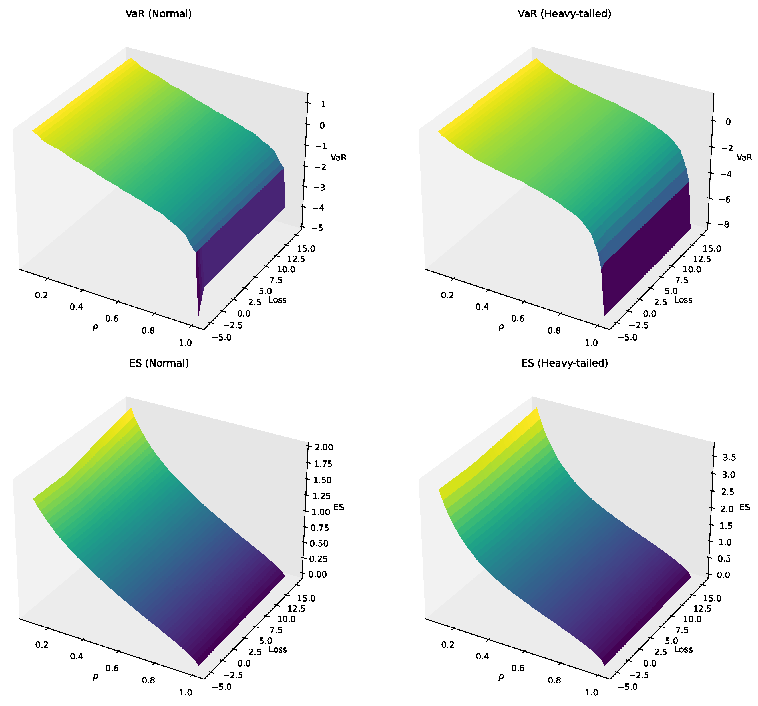
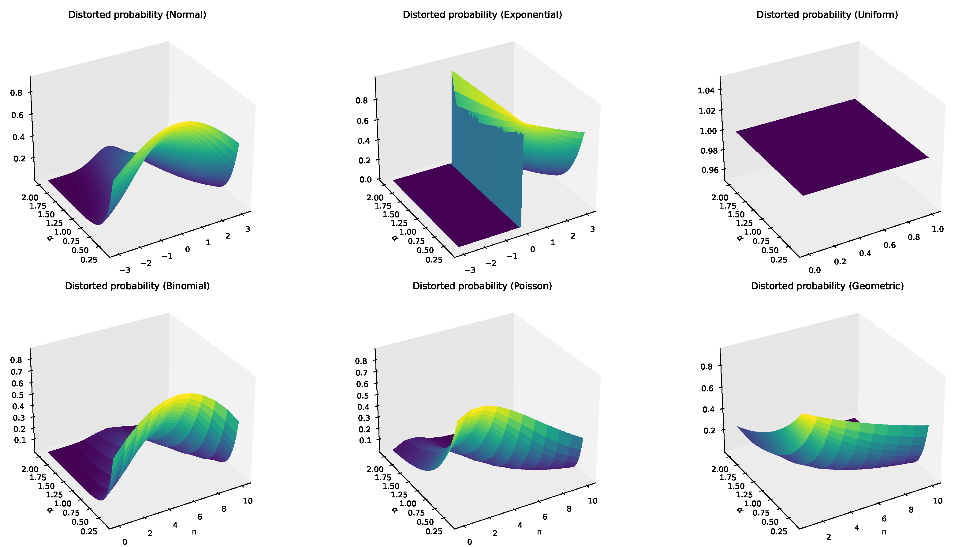
We have three scenarios to set the parameters of distortion functions in Lemma 2. Scenario 1 ($p_1=0.90,p_2=0.95,h_1=0.5$) places relatively moderate weight on losses up to the 90th percentile and higher weight beyond that, with a very high weight on losses beyond the 95th percentile. Scenario 2 ($p_1=0.95,p_2=0.99,h_1=0.3$) places less weight on losses up to the 95th percentile and significantly higher weight beyond the 95th percentile, with the highest weight on losses beyond the 99th percentile. Scenario 3 ($p_1=0.85$, $p_2=0.90,h_1=0.4$) places moderate weight on losses up to the 85th percentile and higher weight beyond that, with the highest weight on losses beyond the 90th percentile.

As shown in Figure 1, by applying the distortion functions to Lemma A1, the SensitivityVaR provides a smoother transition between moderate and extreme risks, reflecting a more nuanced view of potential losses. In comparison, VaR only accounts for risks beyond a certain threshold, ignoring the magnitude of extreme losses. This step-function approach is less effective in capturing the full scope of tail risks. On the other hand, ES provides a continuous weighting of all extreme losses but lacks the flexibility to prioritize specific risk thresholds. By combining the strengths of both VaR and ES, SensitivityVaR offers superior tail risk management. This is particularly advantageous in portfolios with carbon-intensive assets, where the likelihood of extreme events (such as regulatory shocks or market disruptions) is higher. The inclusion of distortion functions enables SensitivityVaR to adjust dynamically to these risks, ensuring a more robust risk management strategy.

Let $X=(X_1,X_2,\dots ,X_n)$ represent the returns of assets, where the asset is associated with carbon intensity, and let Z be a scalar sample to be predicted. We are interested in the coverage probability of Z using SensitivityVaR, targeting a coverage probability level $p\in (0,1)$. For simplicity, assume X and Z are distributed independently and identically from a probability function $f_Z(x;\mathit{\theta })$, parameterized by $\mathit{\theta }$. The cumulative distribution function of the loss variable X is denoted by $F_X(x;\mathit{\theta })$. The p-quantile for the distribution is given by $z_p(\mathit{\theta })=F^{-1}(p;\mathit{\theta })$. Since $\mathit{\theta }$ is generally unknown, we use an estimator $\widehat{\mathit{\theta }}=\widehat{\mathit{\theta }}(X)$ based on the sample X. The p-quantile based on $\widehat{\mathit{\theta }}$ is denoted as $z_p(\widehat{\mathit{\theta }})$. For SensitivityVaR, we combine the Cornish–Fisher adjusted VaR and ES. The estimative limits for VaR and ES are denoted by ${\mathrm{VaR}}_{p_1,\widehat{\mathit{\theta }}}^{{\mathrm{CF}}_{\mathcal{N}}}(X)$ and ${\mathrm{ES}}_{p_2,\widehat{\mathit{\theta }}}^{{\mathrm{CF}}_{\mathcal{T}}}(X)$. Given $\widehat{\mathit{\theta }}$, the coverage probability can be expressed as

$$\begin{array}{c}\hfill \mathbb{P}\left(Z{\le }^{\mathrm{CF}}{\mathrm{SensitivityVaR}}_{p_1,p_2,\widehat{\mathit{\theta }}}^{h_1,h_2}(X)\right)={\mathbb{E}}_{X;\omega }\left[F_Z\left({}^{\mathrm{CF}}\mathrm{SensitivityVaR}_{p_1,p_2,\widehat{\mathit{\theta }}}^{h_1,h_2}(X)\right)\right],\end{array}$$

where

$${}^{\mathrm{CF}}\mathrm{SensitivityVaR}_{p_1,p_2,\widehat{\mathit{\theta }}}^{h_1,h_2}(X)=h_1·{\mathrm{VaR}}_{p_1,\widehat{\mathit{\theta }}}^{{\mathrm{CF}}_{\mathcal{N}}}(X)+h_2·{\mathrm{ES}}_{p_2,\widehat{\mathit{\theta }}}^{{\mathrm{CF}}_{\mathcal{T}}}(X),$$

and

$$h_1={\displaystyle \frac{1-p_2}{1-p_1}},h_2={\displaystyle \frac{p_2-p_1}{1-p_1}}.$$

Assuming $\sqrt{n}$-consistency of the estimator $\widehat{\mathit{\theta }}$, the coverage probability of Equation (4) can be approximated by

$$\mathbb{P}\left(Z{\le }^{\mathrm{CF}}{\mathrm{SensitivityVaR}}_{p_1,p_2,\widehat{\mathit{\theta }}}^{h_1,h_2}(X)\right)=p_2+O(n^{-1}).$$

This formulation highlights the robustness of SensitivityVaR in terms of coverage probability. A robust measure in this context ensures that the coverage probability closely aligns with the target level $p_2$, even under varying sample conditions and potential model misspecifications.

2.3. Simulation Results and Statistical Analysis

We design Algorithm 1 to simulate the coverage probabilities of SensitivityVaR under different return distributions, including both normal and fat-tailed distributions. The Cornish–Fisher expansion allows SensitivityVaR to adapt to skewed and kurtotic return distributions, which are common in real-world financial markets. By simulating the coverage probabilities for both normal and Student’s t-distributions, the algorithm demonstrates that SensitivityVaR consistently provides accurate estimates of tail risks. This consistency is critical for hedging, as it ensures that risk predictions align closely with actual outcomes, particularly in periods of market stress.

Algorithm 1 Coverage Probability for SensitivityVaR

1: Input: Number of simulations N, sample size n, confidence levels $p_1$ and $p_2$, parameter distribution $\mathit{\theta }$ 2: Output: Coverage probability for SensitivityVaR 3: function CornishFisherVaR($X,p_1$) 4: $q_{p_1,\mathit{\theta }}\leftarrow {\Phi }_{\mathit{\theta }}^{-1}(p_1)$ {Standard normal quantile} 5: $\gamma \leftarrow \mathrm{skewness}(X_C)$ 6: $\delta \leftarrow \mathrm{kurtosis}(X_C)$ 7: $q_{p_1;\mathit{\theta }}^{{\mathrm{CF}}_{\mathcal{N}}}\leftarrow q_{p_1;\mathit{\theta }}+{\displaystyle \frac{1}{6}}(q_{p_1;\mathit{\theta }}^2-1)·\gamma +{\displaystyle \frac{1}{24}}(q_{p_1;\mathit{\theta }}^3-3q_{p_1;\mathit{\theta }})·\delta -{\displaystyle \frac{1}{36}}(2q_{p_1;\mathit{\theta }}^3-5q_{p_1;\mathit{\theta }})·{\gamma }^2$ 8: return ${\mu }_{X_C}+{\sigma }_{X_C}·{\mathrm{q}}_{p_1;\mathit{\theta }}^{{\mathrm{CF}}_{\mathcal{N}}}$ 9: end function 10: function CornishFisherES($X_C,p_2$) 11: $q_{p_2,\nu ,\mathit{\theta }}\leftarrow t_{\mathit{\theta }}^{-1}(p_2,\nu =3)$ {t-distribution quantile} 12: $\gamma \leftarrow \mathrm{skewness}(X)$ 13: $\delta \leftarrow \mathrm{kurtosis}(X)$ 14: $q_{p_2,\nu ,\mathit{\theta }}^{{\mathrm{CF}}_{\mathcal{T}}}\leftarrow q_{p_2,\nu ;\mathit{\theta }}+{\displaystyle \frac{1}{6}}(q_{p_2,\nu ;\mathit{\theta }}^2-1)·\gamma +{\displaystyle \frac{1}{24}}(q_{p_2,\nu ;\mathit{\theta }}^3-3t_{p_2,\nu })·\delta -{\displaystyle \frac{1}{36}}(2q_{p_2,\nu ;\mathit{\theta }}^3-5q_{p_2,\nu ;\mathit{\theta }})·{\gamma }^2$ 15: return ${\mu }_X+{\sigma }_X·q_{p_2,\nu ,\mathit{\theta }}^{{\mathrm{CF}}_{\mathcal{T}}}$ 16: end function 17: function SensitivityVaR($X,p_1,p_2$) 18: ${\mathrm{VaR}}_{p_1}\leftarrow \mathrm{percentile}(X,p_1·100)$ 19: ${\mathrm{ES}}_{p_2}\leftarrow {\displaystyle \frac{1}{1-p_2}}{\sum }_{X_i\ge {\mathrm{VaR}}_{p2}}{X}_i$ 20: $h_1\leftarrow {\displaystyle \frac{1-p_2}{1-p_1}}$ 21: $h_2\leftarrow {\displaystyle \frac{p_2-p_1}{1-p_1}}$ 22: return $h_1·{\mathrm{VaR}}_{p_1}+h_2·{\mathrm{ES}}_{p_2}$ 23: end function 24: $coverage\_count\leftarrow 0$ 25: for$i\leftarrow 1$ to N 26: $X\leftarrow \mathrm{GenerateSample}(n,\mathrm{distribution}\mathrm{type})$ 27: ${\mathrm{VaR}}_{p_1}^{{\mathrm{CF}}_{\mathcal{N}}}\leftarrow \mathrm{CornishFisherVaR}(X,p_1)$ 28: ${\mathrm{ES}}_{p_2}^{{\mathrm{CF}}_{\mathcal{T}}}\leftarrow \mathrm{CornishFisherES}(X,p_2)$ 29: ${\mathrm{SensitivityVaR}}_{p_1,p_2}^{h_1,h_2}\leftarrow h_1·{\mathrm{VaR}}_{p_1}^{{\mathrm{CF}}_{\mathcal{N}}}+h_2·{\mathrm{ES}}_{p_2}^{{\mathrm{CF}}_{\mathcal{T}}}$ 30:      if ${\displaystyle \frac{1}{n}}{\sum }_{j=1}^n{\mathbb{1}}_{\{X_j\le {\mathrm{SensitivityVaR}}_{p_1,p_2}^{h_1,h_2}\}}\ge p_2$ then 31:            $coverage\_count\leftarrow coverage\_count+1$ 32:      end if 33: end for 34: return ${\displaystyle \frac{coverage\_count}{N}}=0$

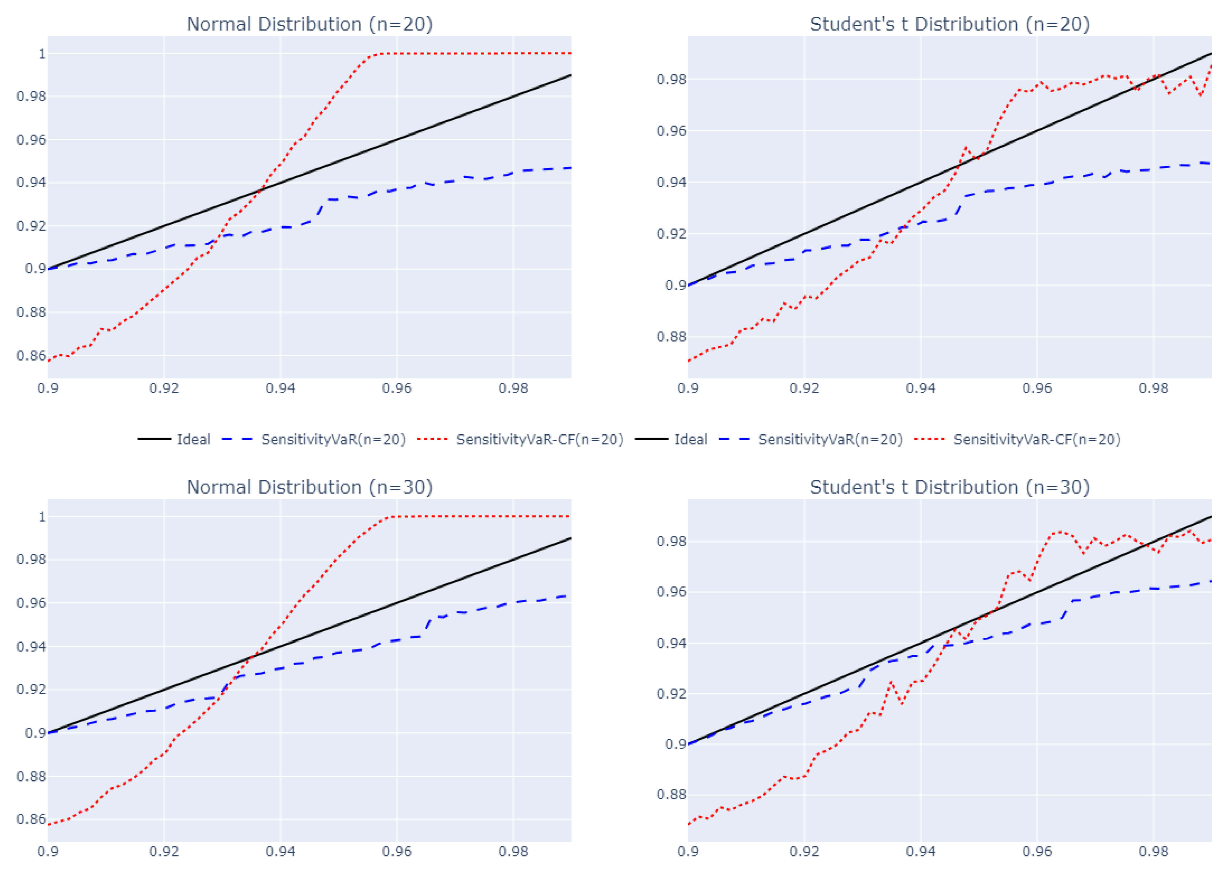
According to Figure 2, for the normal distribution, the ^CF$\mathrm{SensitivityVaR}$ generally shows higher coverage probabilities than the SensitivityVaR. This indicates that the Cornish–Fisher adjustments improve the prediction accuracy for the normal distribution, especially for larger sample sizes. For the Student’s t distribution, the ^CF$\mathrm{SensitivityVaR}$ still tends to perform better than the SensitivityVaR. The advantage of using Cornish–Fisher adjustments is more evident in larger sample sizes, where the red dotted line is closer to the ideal line than the blue dashed line. In some cases, the ^CF$\mathrm{SensitivityVaR}$ performs slightly better or on par with the SensitivityVaR. ^CF$\mathrm{SensitivityVaR}$ tends to provide better or comparable coverage probabilities, indicating more accurate risk predictions in most scenarios, especially with normal and Student’s t distributions.

We simulated SensitivityVaR values using two different return distributions, the normal and Student’s t distribution with three degrees of freedom, to assess the robustness of the risk measure. The simulation results demonstrate that SensitivityVaR behaves differently under light-tailed (normal) and heavy-tailed (Student’s t) distributions. For the normal distribution, the mean SensitivityVaR was approximately 0.0466 with a standard deviation of 2.35. This indicates that the risk measure fluctuates more when dealing with returns that follow a normal distribution, as the thinner tails of the normal distribution do not heavily emphasize extreme losses. The variability in SensitivityVaR reflects the distribution’s tendency to capture moderate risks without being overly sensitive to tail risks. In contrast, the mean SensitivityVaR for the Student’s t distribution was 0.0028, with a much smaller standard deviation of 0.332. The heavy tails of the Student’s t distribution, which place more weight on extreme losses, result in a more conservative and stable risk estimate. The Cornish–Fisher expansion, applied in this context, adjusts the SensitivityVaR to account for the distribution’s skewness and kurtosis, ensuring that the measure remains stable even in the presence of extreme market events. The smaller standard deviation indicates that SensitivityVaR provides a consistent and reliable risk measure under heavy-tailed conditions, where extreme risks are more pronounced. These findings underscore the flexibility of SensitivityVaR to adapt to varying market conditions, demonstrating that it can handle both moderate risks (normal distribution) and extreme risks (Student’s t distribution) effectively. The next section applies SensitivityVaR to portfolio decarbonization strategies, demonstrating its effectiveness in aligning financial returns with carbon reduction goals.

3. Strategies for Portfolio Decarbonization

Carbon intensity refers to the amount of carbon dioxide (CO₂) emissions produced per unit of energy or economic output. It is commonly used as a metric to measure the environmental impact of energy production and consumption. The lower the carbon intensity, the less CO₂ is emitted for each unit of energy produced or economic activity, indicating a cleaner or more efficient process. Carbon intensity in economic activity measures the amount of CO₂ emissions per unit of GDP, often expressed as metric tons of CO₂ per million dollars of GDP (Mt CO₂/USD million GDP). Scopes in carbon emissions refer to the categorization of greenhouse gas (GHG) emissions as defined by the Greenhouse Gas Protocol (ghgprotocol.org). These scopes are used to identify and measure the sources of emissions within an organization or project. There are three scopes:

(i)

Scope 1 (direct emissions): These are direct emissions from sources that are owned or controlled by the company. Examples include emissions from combustion in owned or controlled boilers, furnaces, vehicles, and emissions from chemical production in owned or controlled process equipment.

(ii)

Scope 2 (indirect emissions from energy consumption): These are indirect emissions from the generation of purchased electricity, steam, heating, and cooling consumed by the reporting company. While the emissions occur at the facility where the electricity is generated, they are accounted for in the reporting company’s GHG inventory because they are a result of the company’s energy use.

(iii)

Scope 3 (other indirect emissions): These are all other indirect emissions that occur in the value chain of the reporting company, including both upstream and downstream emissions. Examples include emissions from business travel, procurement, waste, and water, emissions from the production of purchased goods and services, transportation and distribution, and the use of sold products and services.

The carbon intensity of company i with respect to scope j is a normalization of the carbon emission, ${\mathcal{I}}_{i,j}={\displaystyle \frac{{\mathcal{E}}_{i,j}}{Y_i}},$ where $Y_i$ is an output indicator measuring its activity and ${\mathcal{E}}_{i,j}$ is the company’s absolute scope j emissions. Let us consider a portfolio x investing in n assets. Its carbon emissions are equal to ${\mathcal{I}}_j(x)={\sum }_{i=1}^n{w}_i{\mathcal{I}}_{i,j}.$ Typically, revenues (in dollars) are utilized to calculate carbon intensities. It is illogical to compare the carbon emissions of an entity like a football club with a petroleum company due to their vastly different economic scales. This disparity underscores the preference for carbon intensity measures over carbon emission measures in portfolio management. 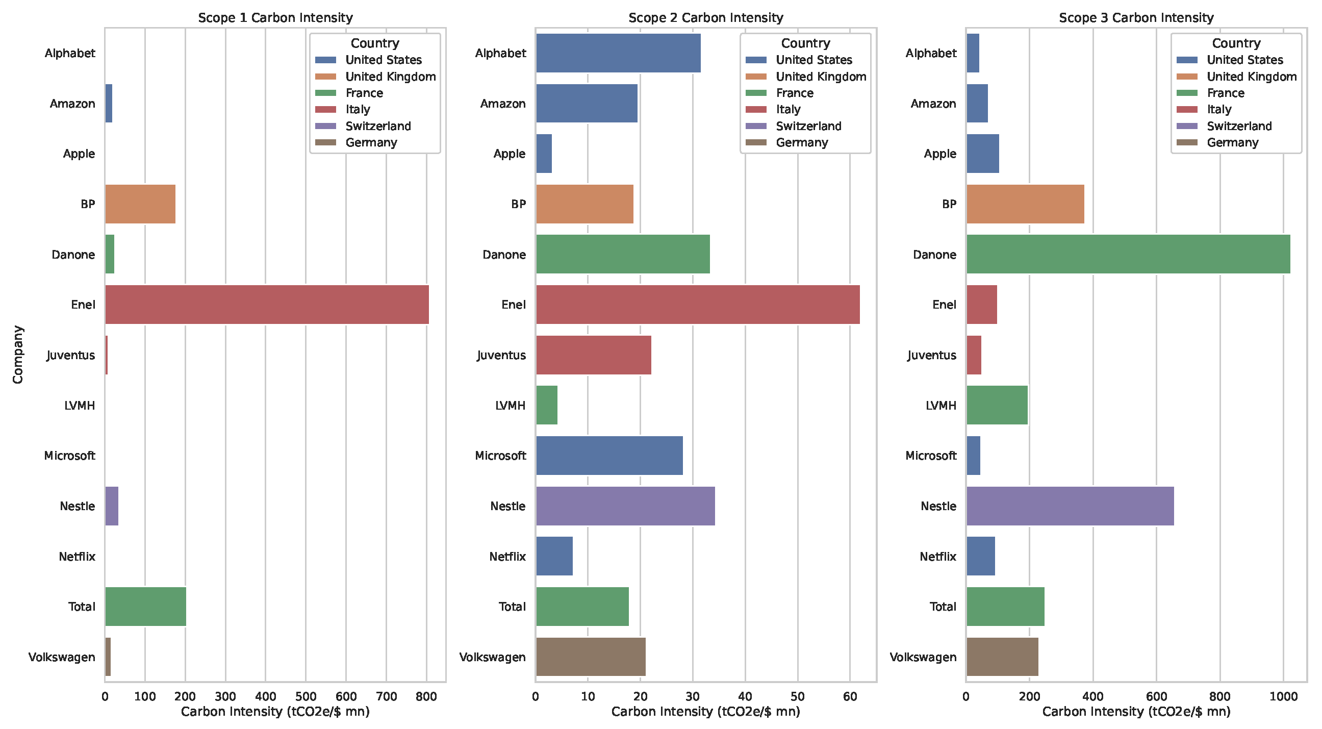Figure 3 represents the carbon intensity of different companies categorized by their respective industries.

In the modern investment landscape, portfolio decarbonization has emerged as a critical strategy for aligning financial goals with environmental sustainability. This approach seeks to reduce the carbon footprint of investment portfolios, thereby contributing to global efforts to mitigate climate change. The integration of carbon intensity metrics into portfolio optimization models enables investors to balance conventional financial objectives with the imperative of reducing carbon emissions. By incorporating carbon data, such as Scope 1, Scope 2, and Scope 3 emissions, investors can make informed decisions that promote sustainability without compromising on returns. The portfolio model we consider involves a comprehensive set of 13 prominent global stocks, Figure 3. These stocks include major technology firms like Apple Inc. (AAPL), Amazon.com Inc. (AMZN), Alphabet Inc. (GOOGL), and Microsoft Corp. (MSFT), along with significant players in other sectors, such as BP p.l.c. (BP) in energy, Danone S.A. (DANOY) in consumer goods, and Volkswagen AG (VWAGY) in the automotive industry. These sectors were deliberately chosen for their relevance to both carbon emissions and financial performance, providing a representative view of how portfolio decarbonization can be achieved across industries. While the majority of companies are based in the US and Europe, they represent global market leaders whose operations and emissions have far-reaching impacts. These companies are crucial players in global decarbonization efforts, which makes them suitable candidates for this analysis. Future research could expand the geographical scope to include more companies from emerging markets to broaden the global relevance.

The selected companies reflect a diverse range of market sectors chosen to highlight the balance between financial performance and decarbonization goals. The selection prioritizes companies with significant global impact and leadership in their respective industries, allowing for a focused analysis of decarbonization strategies in both high-emission and low-emission sectors. These companies were carefully chosen to represent major global players in critical sectors such as technology, energy, and consumer goods, with emissions data covering Scope 1 (direct emissions), Scope 2 (indirect emissions from energy use), and Scope 3 (value chain emissions). This comprehensive emissions coverage ensures that the analysis captures the full spectrum of carbon reduction challenges faced by different industries. The risk of sectoral bias, particularly the influence of high-emission stocks like BP and TTE, is mitigated by incorporating tech giants such as Apple, Microsoft, and Google, which have lower carbon intensities and represent growing sectors with significant investment potential. The inclusion of these diverse sectors ensures that the portfolio’s decarbonization strategy captures the dynamics between carbon-heavy and lower-emission industries, offering a more balanced perspective.

The mean return of each asset i, ${\mu }_i$, is calculated as the average of its historical returns, ${\mu }_i={\displaystyle \frac{1}{T}}{\sum }_{t=1}^T{R}_{i,t},$ where $R_{i,t}$ represents the return of asset i at time t, and T is the number of time periods. The portfolio’s overall expected return is then determined based on these individual asset returns, combined according to their respective weights in the portfolio. The objective of the optimization process is to maximize the portfolio’s adjusted risk–return using the SensitivityVaR, ensuring that the resulting portfolio is both financially efficient and aligned with specific constraints related to returns, carbon intensity, and the first- and second-order distorted stochastic dominance (DFSD and DSSD). The optimization can be mathematically expressed as

$$\underset{w}{max}\left({\displaystyle \frac{{\sum }_{i=1}^n{w}_i{\mu }_i}{{}^{\mathrm{CF}}\mathrm{SensitivityVaR}}}\right),$$

The choice of $p_1$ and $p_2$ significantly impacts the SensitivityVaR calculation. These parameters are optimized by performing a grid search over a range of values to find the combination that maximizes the adjusted risk–return for the portfolio. The portfolio optimization process includes several critical constraints. Firstly, the budget constraint ensures that the total allocation of weights across all assets sums to 100%, formally represented as ${\sum }_{i=1}^n{w}_i=1.$ Secondly, the return constraint ensures that the portfolio’s expected return meets or exceeds a target return, expressed as

$$\sum _{i=1}^n{w}_i·{\mu }_i\ge X_{\mathrm{target}}.$$

Thirdly, the carbon intensity constraint ensures that the portfolio’s carbon footprint does not exceed a specified threshold, formulated as

$$\sum _{i=1}^n{w}_i·{\mathcal{I}}_i^{\mathrm{total}}\le {\mathcal{I}}_{\mathrm{threshold}},$$

where ${\mathcal{I}}_i^{\mathrm{total}}$ is the total carbon intensity from various combination scopes (scope 1, 2, and 3). Finally, the DFSD constraint requires that the SensitivityVaR Equation (4) of our portfolio $P_A=P_{X_1,X_2}^w$ is less than or equal to that of a benchmark portfolio $P_B=P_{X_3,X_4}^w$, or $F_{P_A}{⪰}_1{G}_{P_B}$, ensuring that

$${}^{\mathrm{CF}}\mathrm{SensitivityVaR}(P_A){\le }^{\mathrm{CF}}\mathrm{SensitivityVaR}(P_B).$$

Incorporating the DSSD constraint alongside DFSD provides an additional layer of risk management (see Appendix A for details on stochastic dominance). To incorporate DSSD with SensitivityVaR, the portfolio must not only satisfy the first-order stochastic dominance but also adhere to second-order dominance criteria. The DSSD constraint requires that the area under the distorted distribution function of portfolio $P_A$, $F_{P_A}$, up to any point x, is less than or equal to that under the distorted distribution function of portfolio $P_B$, $F_{P_B}$. This condition ensures that portfolio $P_A$ does not dominate $P_B$ in terms of cumulative distributions, adding conservatism to the portfolio construction process.

Lemma 3.

According to Equation (A2), the second-order distorted stochastic dominance (DSSD) for portfolio decarbonization can be written as

$$\begin{array}{cc}\hfill P_A{⪯}_2{P}_B& \iff {\int }_0^d{g}_{p_1,p_2}^{h_1,h_2}(F_{P_A}(t))dt\le {\int }_0^d{g}_{p_1,p_2}^{h_1,h_2}(F_{P_B}(t))dt\hfill \\ \hfill & \iff \mathbb{E}\left({\left({\tilde{P}}_A-d\right)}_{-}\right)\ge \mathbb{E}\left({\left({\tilde{P}}_B-d\right)}_{-}\right),\hfill \end{array}$$

where $d\in {\mathbb{R}}^{+}$, $g(·)$ is a distortion function as defined in Equation (4), and

$$\begin{array}{c}\hfill \mathbb{E}\left({\left({\tilde{P}}_A-d\right)}_{-}\right)=d-{\int }_0^{d}g\left({\overline{F}}_{P_{X_{{\mathcal{I}}_1},X_{{\mathcal{I}}_2}}^w}(t)\right)dt.\end{array}$$

By integrating the DSSD constraint, the portfolio optimization process can effectively manage not only immediate risks but also the distribution of risks over time, ensuring a more balanced and sustainable portfolio. This dual approach of employing both DFSD and DSSD constraints within the SensitivityVaR framework offers a comprehensive risk management strategy that aligns with environmental, social, and governance (ESG) criteria.

In the following sections, we present the results of the empirical analysis, focusing on the risk–return trade-offs achieved by SensitivityVaR across various portfolio configurations. These findings underscore the measure’s effectiveness in managing tail risks and reducing carbon intensity, paving the way for more sustainable investment strategies.

4. Empirical Analysis and Results

This section presents the empirical analysis and results obtained from the portfolio optimization models applied to a diverse set of 13 stock tickers, as described earlier: ’AAPL’, ’AMZN’, ’GOOGL’, ’BP’, ’MSFT’, ’DANOY’, ’ENLAY’, ’JUVE.MI’, ’LVMUY’, ’NFLX’, ’NSRGY’, ’TTE’, and ’VWAGY’. Historical stock price data were retrieved from Yahoo Finance, covering the period from 1 January 2023 to 31 December 2023 (Yahoo Finance 2024). The optimization models explored are the sustainable enhanced strategy, incorporating Distorted First Stochastic Dominance (DFSD) and Distorted Second Stochastic Dominance (DSSD) constraints with a SensitivityVaR measure, and the conventional variance minimization strategy, which primarily focuses on minimizing portfolio variance without considering these sophisticated risk-adjustment techniques or specific carbon intensity thresholds mandated by global sustainability goals.

The carbon intensity data for each company, covering Scope 1, Scope 2, and Scope 3 emissions, were manually inputted based on Trucost reporting for the year 2019. The 2019 data serve as a strong baseline for this analysis, as many companies set their long-term carbon reduction targets in alignment with the Paris Agreement, which began in that year. Using these metrics provides a reliable reference point to assess progress and implement decarbonization strategies in line with global sustainability goals. To align with global sustainability targets, the portfolio models integrate these carbon intensities into their constraints by combining them into various categories: Scope 1 + Scope 2, Scope 1 + Scope 3, Scope 2 + Scope 3, and Scope 1 + Scope 2 + Scope 3. The target return ($X_{\mathrm{target}}$) is calculated as the mean of historical returns across all tickers, while the carbon intensity threshold is determined using the Paris Agreement’s guideline, reducing carbon intensity by 7% annually from 2019 to 2050. The base carbon intensity is adjusted as follows:

$${\mathcal{I}}_{\mathrm{threshold}(2023)}={\mathcal{I}}_{\mathrm{base}}\times {(0.93)}^4,$$

where ${\mathcal{I}}_{\mathrm{base}}$ represents the base carbon intensity from 2019.

The application of DFSD and DSSD constraints effectively mitigates tail risks by limiting the portfolio’s exposure to extreme market events, especially in high-carbon-intensive assets such as BP and TTE. This approach ensures that the portfolio not only adheres to sustainability goals but also remains resilient to potential market shocks, as highlighted in several studies on sustainable finance and portfolio risk management (e.g., Balbás et al. (2009); Sereda et al. (2010)). These constraints ensure that the portfolio is not overly exposed to tail risks, which are particularly relevant for these stocks given their substantial carbon emissions (see in Figure 3) and market volatility. Conversely, the conventional strategy exhibits a different risk–return profile, characterized by broader risk exposure across the portfolio. The absence of DFSD and DSSD constraints allows for a more varied distribution of risks, as seen in stocks such as AAPL and MSFT, where the risk–return trade-offs are less controlled. The risk, in this case, is simply the variance of returns, which does not capture the full spectrum of potential tail risks. This results in portfolios that may achieve lower overall risk (in terms of variance) but potentially at the cost of higher exposure to extreme market events. For example, AMZN and GOOGL in this strategy show higher expected returns with comparatively higher risks, indicating that without DFSD and DSSD, the portfolio is more susceptible to market fluctuations.

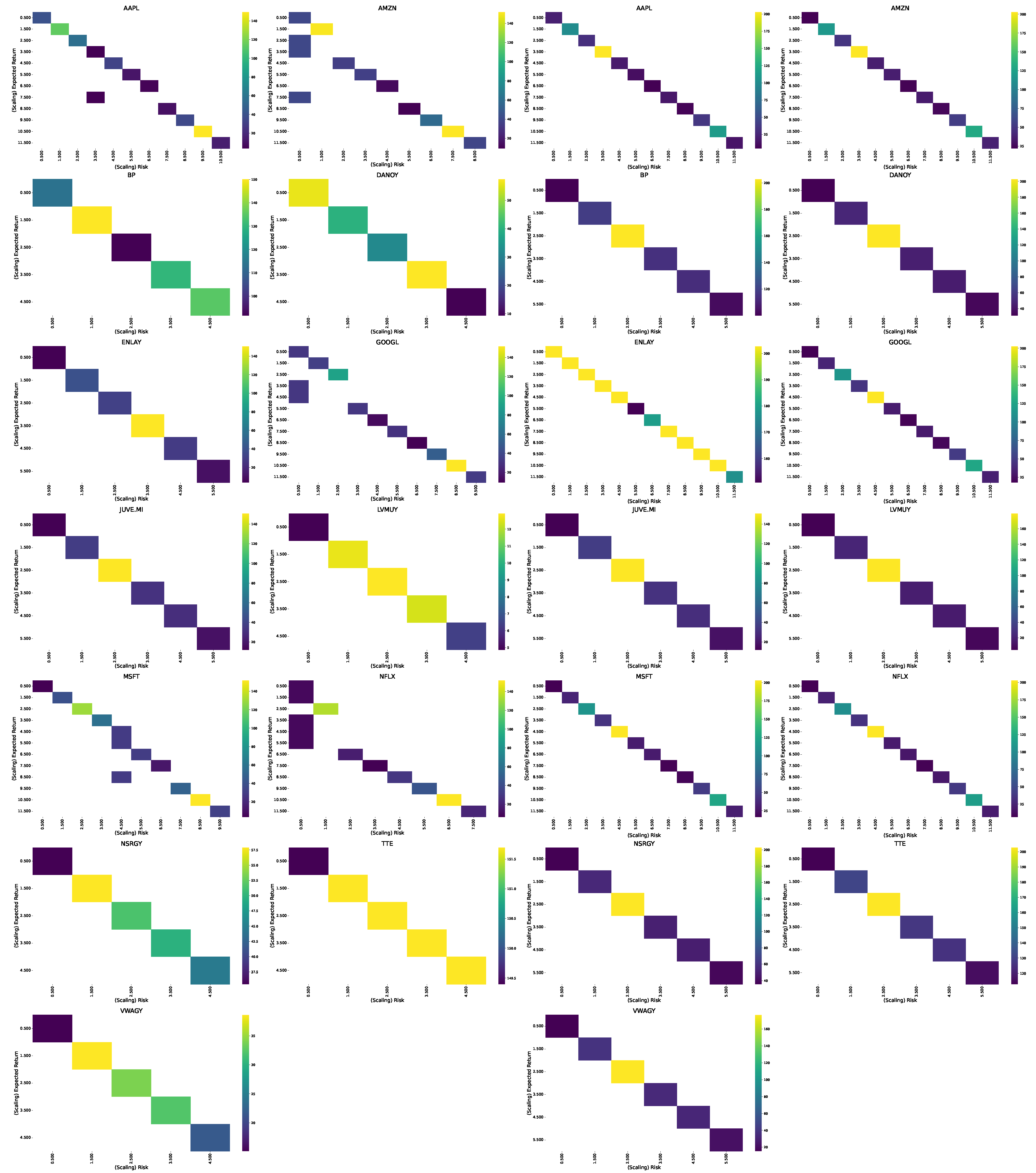
The scatterplot in Figure 4 highlights the differences between the conventional and sustainable portfolios, showcasing the superior risk–return balance achieved through sustainable investing strategies. This scatterplot illustrates the analysis of ^CF$\mathrm{SensitivityVaR}$ and expected return provides a clear understanding of the portfolios’ performance. The sustainable approach consistently achieves higher returns without substantially increasing risk, reflecting the enhanced risk management and sustainability-focused strategies employed. From Figure 5, it is evident that the sustainable strategy generally achieves a more favorable risk–return profile across the various asset combinations. For instance, combinations involving ’AAPL’ with ’GOOGL’ or ’AMZN’ under this strategy display higher expected returns with moderate risk compared to the conventional strategy. This suggests that incorporating DFSD and DSSD constraints effectively enhances portfolio performance by penalizing higher-risk and higher-carbon intensity assets, thereby encouraging a more sustainable investment approach.

The carbon intensity heatmaps, Figure 6, provide further insights into the efficacy of these two strategies. In the sustainable strategy, the carbon intensity across portfolios is managed with precision, reflecting a strict adherence to the thresholds derived from the Paris Agreement. Research on decarbonization strategies in portfolio optimization has demonstrated similar outcomes, where reducing carbon intensity can be achieved without sacrificing financial performance (e.g., Amundi Research Center (2022); Cheema-Fox et al. (2019)). This approach results in a gradual and controlled color gradient across the heatmaps, particularly in high-emission stocks like BP, ENLAY (Enel Americas S.A.), and DANOY (see Figure 3). The strategy’s ability to incorporate carbon intensity constraints effectively reduces the overall carbon footprint of the portfolio, ensuring that even high-return portfolios maintain environmental sustainability. In contrast, the conventional strategy exhibits a more erratic pattern in carbon intensity management. The heatmaps for this strategy show abrupt transitions in color, indicating less nuanced control over carbon emissions. For instance, stocks like NSRGY (Nestlé S.A.) and VWAGY display significant carbon intensity in certain combinations, reflecting the strategy’s limited capacity to balance carbon reduction goals with risk-adjusted returns maximization. This lack of stringent carbon management might lead to portfolios that, while optimized for variance, do not align with long-term sustainability targets.

By incorporating DFSD and DSSD, the sustainable strategy actively mitigates the risk of large drawdowns and extreme market events, which are more prevalent in carbon-intensive sectors. This risk mitigation approach reduces the likelihood of significant financial losses while maintaining a commitment to decarbonization. For example, combinations involving MSFT and GOOGL are prevalent, as these stocks offer relatively lower carbon footprints and stable returns. On the other hand, the conventional strategy allows for more flexibility, often leading to portfolios that include riskier, higher carbon-emitting stocks such as BP and TTE. However, these portfolios may achieve higher short-term returns at the expense of increased exposure to environmental and market risks.

Figure 5. This figure compares the risk–return profiles of sustainable (left) and conventional (right) strategies across various asset combinations, highlighting how the sustainable strategy, with DFSD and DSSD constraints, leads to improved risk management. The sustainable portfolios show more controlled risk exposure, particularly in carbon-intensive assets like BP and TTE, while conventional portfolios exhibit broader risk exposure.

Figure 5. This figure compares the risk–return profiles of sustainable (left) and conventional (right) strategies across various asset combinations, highlighting how the sustainable strategy, with DFSD and DSSD constraints, leads to improved risk management. The sustainable portfolios show more controlled risk exposure, particularly in carbon-intensive assets like BP and TTE, while conventional portfolios exhibit broader risk exposure.

Figure 6. Carbon intensity heatmaps for various asset combinations, comparing sustainable (left) and conventional (right) strategies. The sustainable strategy demonstrates controlled carbon intensity, with gradual color transitions reflecting adherence to decarbonization goals. In contrast, the conventional strategy exhibits more variability, indicating less effective carbon management, especially in high-emission stocks like BP, Enel, and Nestlé.

Figure 6. Carbon intensity heatmaps for various asset combinations, comparing sustainable (left) and conventional (right) strategies. The sustainable strategy demonstrates controlled carbon intensity, with gradual color transitions reflecting adherence to decarbonization goals. In contrast, the conventional strategy exhibits more variability, indicating less effective carbon management, especially in high-emission stocks like BP, Enel, and Nestlé.

5. Discussion

The portfolio decarbonization model presented in this study aims to achieve an optimal balance between financial performance, risk management, and sustainability. By integrating the SensitivityVaR measure with Distorted First Stochastic Dominance (DFSD) and Distorted Second Stochastic Dominance (DSSD) constraints, the model offers a comprehensive framework that not only targets superior risk-adjusted returns but also aligns with environmental sustainability goals. The addition of DFSD and DSSD constraints significantly impacts the distribution of carbon intensity, emphasizing the trade-offs involved in sustainable portfolio management. Incorporating sustainability constraints can help mitigate the typical trade-off between return and carbon intensity, offering a pathway to achieving higher returns with a lower environmental impact. In addition to the short-term performance discussed, it is crucial to consider the long-term impacts of climate risks on portfolio returns. Changes in regulations, evolving carbon taxes, and shifts in consumer preferences toward sustainability are expected to create significant financial risks and opportunities in the coming decades. Portfolios that are heavily invested in carbon-intensive sectors may face increasing costs and reduced profitability as stricter emissions regulations are imposed. Conversely, portfolios aligned with sustainable investment strategies, such as the ones developed in this study, may benefit from reduced exposure to these risks and improved resilience to future climate-related shocks. Future research could extend this work by incorporating long-term climate scenarios, including carbon pricing and evolving regulatory environments, into the portfolio decarbonization model. These findings align with broader research in sustainable finance and risk management, where distortion risk measures such as GlueVaR have been shown to enhance risk-adjusted performance (e.g., Belles-Sampera et al. (2014)). Furthermore, tail risk measures, such as those discussed by Zhu and Li (2012), are valuable for managing extreme risks, which is crucial when incorporating sustainability constraints. AMZN’s results further illustrate this difference, where the sustainable strategy manages to maintain higher expected returns with relatively moderate carbon intensities compared to the conventional strategy, which shows a steeper increase in carbon intensity with rising returns. This indicates that the DFSD and DSSD constraints help in balancing financial performance with carbon intensity reduction, offering a more sustainable investment approach. BP, a conventionally high-carbon asset, exhibits a complex pattern in both strategies.

The sustainable strategy, while maintaining lower carbon intensities, manages to achieve moderate returns, indicating a more nuanced trade-off between risk, return, and sustainability. The conventional strategy, however, struggles to balance these factors, often resulting in higher carbon intensities for marginally higher returns. GOOGL’s results further highlight the benefits of the sustainable strategy, where the highest returns are achieved with moderate increases in carbon intensity. The conventional strategy, in contrast, often leads to higher carbon intensities for similar levels of return, reflecting its lesser emphasis on environmental impact. The sustainable strategy demonstrates that achieving desirable returns with controlled carbon intensities is possible, making it a promising option for responsible investing. As global climate regulations tighten, portfolios are increasingly exposed to regulatory and reputational risks. Investors and companies face growing pressure to reduce carbon footprints, with potential penalties, market access restrictions, and reputational harm for those not meeting regulatory standards. By incorporating carbon intensity constraints, the sustainable strategy mitigates these risks, aligning portfolios with global decarbonization efforts and enhancing resilience to regulatory shifts. In contrast, conventional strategies often involve a trade-off between higher returns and higher carbon intensities, reinforcing the importance of integrating sustainability measures in modern portfolio management. The sustainable strategy offers a clear advantage in balancing risk, return, and carbon intensity, making it a valuable tool for investors aiming to build resilient, sustainable portfolios. Another key consideration is the cost of trading and rebalancing, which can affect net returns. While the model optimizes for risk, return, and carbon intensity, it does not account for transaction costs. High-turnover strategies, in particular, may see performance erosion over time due to these costs. Future research should incorporate transaction costs to provide a more realistic evaluation of the strategy’s performance, offering deeper insights into the trade-offs between turnover, cost, and sustainability.

Table A1. Portfolio weights summary for two assets with DSSD constraint and various combinations of Scope 1, 2 and 3.

Scope	Combination	Carbon Intensity	Expected Return	Risk	${\mathit{w}}_1$	${\mathit{w}}_2$
Scope 1 + Scope 2	(’AAPL’, ’AMZN’)	40.1390	0.0024	0.0004	0.0000	1.0000
Scope 1 + Scope 2	(’AAPL’, ’GOOGL’)	32.0740	0.0019	0.0004	0.0000	1.0000
Scope 1 + Scope 2	(’AAPL’, ’BP’)	113.7485	0.0009	0.0001	0.4288	0.5712
Scope 1 + Scope 2	(’AAPL’, ’MSFT’)	3.5080	0.0018	0.0002	1.0000	0.0000
Scope 1 + Scope 2	(’AAPL’, ’DANOY’)	55.9442	0.0009	0.0001	0.0531	0.9469
Scope 1 + Scope 2	(’AAPL’, ’ENLAY’)	3.5080	0.0018	0.0002	1.0000	0.0000
Scope 1 + Scope 2	(’AAPL’, ’JUVE.MI’)	11.9595	0.0009	0.0001	0.6991	0.3009
Scope 1 + Scope 2	(’AAPL’, ’LVMUY’)	4.8651	0.0009	0.0002	0.3173	0.6827
Scope 1 + Scope 2	(’AAPL’, ’NFLX’)	9.3210	0.0022	0.0005	0.0000	1.0000
Scope 1 + Scope 2	(’AAPL’, ’NSRGY’)	35.5030	0.0009	0.0001	0.5039	0.4961
Scope 1 + Scope 2	(’AAPL’, ’TTE’)	149.3958	0.0009	0.0001	0.3328	0.6672
Scope 1 + Scope 2	(’AAPL’, ’VWAGY’)	15.0712	0.0009	0.0001	0.6549	0.3451
Scope 1 + Scope 2	(’AMZN’, ’GOOGL’)	35.5812	0.0022	0.0003	0.4349	0.5651
Scope 1 + Scope 2	(’AMZN’, ’BP’)	150.1755	0.0009	0.0002	0.2963	0.7037
Scope 1 + Scope 2	(’AMZN’, ’MSFT’)	40.1390	0.0024	0.0004	1.0000	0.0000
Scope 1 + Scope 2	(’AMZN’, ’DANOY’)	40.1390	0.0024	0.0004	1.0000	0.0000
Scope 1 + Scope 2	(’AMZN’, ’ENLAY’)	40.1390	0.0024	0.0004	1.0000	0.0000
Scope 1 + Scope 2	(’AMZN’, ’JUVE.MI’)	36.4312	0.0009	0.0002	0.5658	0.4342
Scope 1 + Scope 2	(’AMZN’, ’LVMUY’)	12.6601	0.0009	0.0002	0.2068	0.7932
Scope 1 + Scope 2	(’AMZN’, ’NFLX’)	9.3210	0.0022	0.0005	0.0000	1.0000
Scope 1 + Scope 2	(’AMZN’, ’NSRGY’)	57.8873	0.0009	0.0001	0.3629	0.6371
Scope 1 + Scope 2	(’AMZN’, ’TTE’)	151.6952	0.0012	0.0001	0.3872	0.6128
Scope 1 + Scope 2	(’AMZN’, ’VWAGY’)	38.6246	0.0009	0.0002	0.5156	0.4844
Scope 1 + Scope 2	(’GOOGL’, ’BP’)	91.6142	0.0013	0.0002	0.6379	0.3621
Scope 1 + Scope 2	(’GOOGL’, ’MSFT’)	29.3630	0.0019	0.0002	0.0000	1.0000
Scope 1 + Scope 2	(’GOOGL’, ’DANOY’)	32.0740	0.0019	0.0004	1.0000	0.0000
Scope 1 + Scope 2	(’GOOGL’, ’ENLAY’)	32.0740	0.0019	0.0004	1.0000	0.0000
Scope 1 + Scope 2	(’GOOGL’, ’JUVE.MI’)	31.9124	0.0009	0.0002	0.6597	0.3403
Scope 1 + Scope 2	(’GOOGL’, ’LVMUY’)	12.9236	0.0009	0.0002	0.2795	0.7205
Scope 1 + Scope 2	(’GOOGL’, ’NFLX’)	9.3210	0.0022	0.0005	0.0000	1.0000
Scope 1 + Scope 2	(’GOOGL’, ’NSRGY’)	51.5196	0.0009	0.0001	0.4587	0.5413
Scope 1 + Scope 2	(’GOOGL’, ’TTE’)	151.6952	0.0010	0.0001	0.3707	0.6293
Scope 1 + Scope 2	(’GOOGL’, ’VWAGY’)	33.9860	0.0009	0.0002	0.6129	0.3871
Scope 1 + Scope 2	(’BP’, ’MSFT’)	130.0953	0.0009	0.0001	0.6027	0.3973
Scope 1 + Scope 2	(’BP’, ’NFLX’)	134.9505	0.0009	0.0002	0.6712	0.3288
Scope 1 + Scope 2	(’MSFT’, ’DANOY’)	57.5003	0.0009	0.0001	0.0470	0.9530
Scope 1 + Scope 2	(’MSFT’, ’ENLAY’)	29.3630	0.0019	0.0002	1.0000	0.0000
Scope 1 + Scope 2	(’MSFT’, ’JUVE.MI’)	30.0984	0.0009	0.0002	0.6711	0.3289
Scope 1 + Scope 2	(’MSFT’, ’LVMUY’)	12.4150	0.0009	0.0002	0.2899	0.7101
Scope 1 + Scope 2	(’MSFT’, ’NFLX’)	29.3630	0.0019	0.0002	1.0000	0.0000
Scope 1 + Scope 2	(’MSFT’, ’NSRGY’)	49.7836	0.0009	0.0001	0.4714	0.5286
Scope 1 + Scope 2	(’MSFT’, ’TTE’)	151.6952	0.0010	0.0001	0.3655	0.6345
Scope 1 + Scope 2	(’MSFT’, ’VWAGY’)	32.2320	0.0009	0.0002	0.6250	0.3750
Scope 1 + Scope 2	(’DANOY’, ’NFLX’)	9.3210	0.0022	0.0005	0.0000	1.0000
Scope 1 + Scope 2	(’ENLAY’, ’NFLX’)	9.3210	0.0022	0.0005	0.0000	1.0000
Scope 1 + Scope 2	(’JUVE.MI’, ’NFLX’)	18.1732	0.0009	0.0003	0.3974	0.6026
Scope 1 + Scope 2	(’LVMUY’, ’NFLX’)	6.3864	0.0009	0.0002	0.7672	0.2328
Scope 1 + Scope 2	(’NFLX’, ’NSRGY’)	44.6073	0.0009	0.0001	0.3986	0.6014
Scope 1 + Scope 2	(’NFLX’, ’TTE’)	151.6952	0.0010	0.0002	0.3311	0.6689
Scope 1 + Scope 2	(’NFLX’, ’VWAGY’)	21.6919	0.0009	0.0003	0.5533	0.4467
Scope 1 + Scope 3	(’AAPL’, ’AMZN’)	92.0240	0.0024	0.0004	0.0000	1.0000
Scope 1 + Scope 3	(’AAPL’, ’GOOGL’)	44.7350	0.0019	0.0004	0.0000	1.0000
Scope 1 + Scope 3	(’AAPL’, ’BP’)	151.6952	0.0016	0.0001	0.8984	0.1016
Scope 1 + Scope 3	(’AAPL’, ’MSFT’)	106.3500	0.0018	0.0002	1.0000	0.0000
Scope 1 + Scope 3	(’AAPL’, ’DANOY’)	106.3500	0.0018	0.0002	1.0000	0.0000
Scope 1 + Scope 3	(’AAPL’, ’ENLAY’)	106.3500	0.0018	0.0002	1.0000	0.0000
Scope 1 + Scope 3	(’AAPL’, ’JUVE.MI’)	92.3911	0.0009	0.0001	0.6991	0.3009
Scope 1 + Scope 3	(’AAPL’, ’LVMUY’)	151.6952	0.0011	0.0001	0.5075	0.4925
Scope 1 + Scope 3	(’AAPL’, ’NFLX’)	96.1860	0.0022	0.0005	0.0000	1.0000
Scope 1 + Scope 3	(’AAPL’, ’NSRGY’)	106.3500	0.0018	0.0002	1.0000	0.0000
Scope 1 + Scope 3	(’AAPL’, ’TTE’)	151.6952	0.0018	0.0002	1.0000	0.0000
Scope 1 + Scope 3	(’AAPL’, ’VWAGY’)	151.6952	0.0010	0.0001	0.6774	0.3226
Scope 1 + Scope 3	(’AMZN’, ’GOOGL’)	65.2995	0.0022	0.0003	0.4349	0.5651
Scope 1 + Scope 3	(’AMZN’, ’BP’)	92.0240	0.0024	0.0004	1.0000	0.0000
Scope 1 + Scope 3	(’AMZN’, ’MSFT’)	92.0240	0.0024	0.0004	1.0000	0.0000
Scope 1 + Scope 3	(’AMZN’, ’DANOY’)	92.0240	0.0024	0.0004	1.0000	0.0000
Scope 1 + Scope 3	(’AMZN’, ’ENLAY’)	92.0240	0.0024	0.0004	1.0000	0.0000
Scope 1 + Scope 3	(’AMZN’, ’JUVE.MI’)	78.1001	0.0009	0.0002	0.5658	0.4342
Scope 1 + Scope 3	(’AMZN’, ’LVMUY’)	151.2862	0.0014	0.0002	0.4430	0.5570
Scope 1 + Scope 3	(’AMZN’, ’NFLX’)	96.1860	0.0022	0.0005	0.0000	1.0000
Scope 1 + Scope 3	(’AMZN’, ’NSRGY’)	151.6952	0.0022	0.0003	0.9004	0.0996
Scope 1 + Scope 3	(’AMZN’, ’TTE’)	151.6952	0.0021	0.0003	0.8347	0.1653
Scope 1 + Scope 3	(’AMZN’, ’TTE’)	151.6952	0.0021	0.0003	0.8347	0.1653
Scope 1 + Scope 3	(’AMZN’, ’VWAGY’)	151.6952	0.0012	0.0002	0.6147	0.3853
Scope 1 + Scope 3	(’GOOGL’, ’BP’)	151.6952	0.0016	0.0002	0.7895	0.2105
Scope 1 + Scope 3	(’GOOGL’, ’MSFT’)	48.4010	0.0019	0.0002	0.0000	1.0000
Scope 1 + Scope 3	(’GOOGL’, ’DANOY’)	44.7350	0.0019	0.0004	1.0000	0.0000
Scope 1 + Scope 3	(’GOOGL’, ’ENLAY’)	44.7350	0.0019	0.0004	1.0000	0.0000
Scope 1 + Scope 3	(’GOOGL’, ’JUVE.MI’)	49.9137	0.0009	0.0002	0.6597	0.3403
Scope 1 + Scope 3	(’GOOGL’, ’LVMUY’)	151.6952	0.0009	0.0002	0.3040	0.6960
Scope 1 + Scope 3	(’GOOGL’, ’NFLX’)	96.1860	0.0022	0.0005	0.0000	1.0000
Scope 1 + Scope 3	(’GOOGL’, ’NSRGY’)	151.6952	0.0016	0.0003	0.8345	0.1655
Scope 1 + Scope 3	(’GOOGL’, ’TTE’)	151.6952	0.0015	0.0002	0.7380	0.2620
Scope 1 + Scope 3	(’GOOGL’, ’VWAGY’)	123.0000	0.0009	0.0002	0.6129	0.3871
Scope 1 + Scope 3	(’BP’, ’MSFT’)	151.6952	0.0015	0.0002	0.2048	0.7952
Scope 1 + Scope 3	(’BP’, ’NFLX’)	151.6952	0.0020	0.0004	0.1216	0.8784
Scope 1 + Scope 3	(’MSFT’, ’DANOY’)	48.4010	0.0019	0.0002	1.0000	0.0000
Scope 1 + Scope 3	(’MSFT’, ’ENLAY’)	48.4010	0.0019	0.0002	1.0000	0.0000
Scope 1 + Scope 3	(’MSFT’, ’JUVE.MI’)	52.2004	0.0009	0.0002	0.6711	0.3289
Scope 1 + Scope 3	(’MSFT’, ’LVMUY’)	151.6952	0.0009	0.0002	0.3114	0.6886
Scope 1 + Scope 3	(’MSFT’, ’NFLX’)	48.4010	0.0019	0.0002	1.0000	0.0000
Scope 1 + Scope 3	(’MSFT’, ’NSRGY’)	151.6952	0.0016	0.0002	0.8393	0.1607
Scope 1 + Scope 3	(’MSFT’, ’TTE’)	151.6952	0.0015	0.0002	0.7447	0.2553
Scope 1 + Scope 3	(’MSFT’, ’VWAGY’)	122.8469	0.0009	0.0002	0.6250	0.3750
Scope 1 + Scope 2 + Scope 3	(’AAPL’, ’AMZN’)	111.6300	0.0024	0.0004	0.0000	1.0000
Scope 1 + Scope 2 + Scope 3	(’AAPL’, ’GOOGL’)	76.3490	0.0019	0.0004	0.0000	1.0000
Scope 1 + Scope 2 + Scope 3	(’AAPL’, ’BP’)	151.6952	0.0016	0.0001	0.9090	0.0910
Scope 1 + Scope 2 + Scope 3	(’AAPL’, ’MSFT’)	109.6640	0.0018	0.0002	1.0000	0.0000
Scope 1 + Scope 2 + Scope 3	(’AAPL’, ’DANOY’)	109.6640	0.0018	0.0002	1.0000	0.0000
Scope 1 + Scope 2 + Scope 3	(’AAPL’, ’ENLAY’)	109.6640	0.0018	0.0002	1.0000	0.0000
Scope 1 + Scope 2 + Scope 3	(’AAPL’, ’JUVE.MI’)	101.3866	0.0009	0.0001	0.6991	0.3009
Scope 1 + Scope 2 + Scope 3	(’AAPL’, ’LVMUY’)	151.6952	0.0012	0.0001	0.5486	0.4514
Scope 1 + Scope 2 + Scope 3	(’AAPL’, ’NFLX’)	103.5980	0.0022	0.0005	0.0000	1.0000
Scope 1 + Scope 2 + Scope 3	(’AAPL’, ’NSRGY’)	109.6640	0.0018	0.0002	1.0000	0.0000
Scope 1 + Scope 2 + Scope 3	(’AAPL’, ’TTE’)	109.6640	0.0018	0.0002	1.0000	0.0000
Scope 1 + Scope 2 + Scope 3	(’AAPL’, ’VWAGY’)	151.6952	0.0011	0.0001	0.7346	0.2654

(see Appendix B) highlights the range of portfolio combinations that balance carbon intensity, expected returns, and risk, aligning well with the analysis described. The preference for tech giants like Apple (AAPL), Amazon (AMZN), and Microsoft (MSFT) is evident across various scopes, as these companies consistently appear in different combinations. They often show lower carbon intensities while maintaining competitive risk-adjusted returns, supporting the claim that tech stocks play a crucial role in sustainable portfolios. The inclusion of energy companies like BP and TotalEnergies (TTE) in the tables further underscores the analysis. These combinations exhibit significantly higher carbon intensities, with values reaching up to 151.70. The associated trade-offs in risk-adjusted returns, as mentioned in the analysis, are clearly reflected in the data, illustrating the challenges of integrating carbon-intensive sectors into a sustainable investment strategy. Moreover, the tables feature combinations of tech stocks with companies from less carbon-intensive sectors, such as Nestlé (NSRGY) and LVMH (LVMUY). These portfolios strike a balance by maintaining moderate carbon intensities while offering reasonable returns. This aligns with the narrative in the analysis, which highlights the potential benefits of mixed portfolios that combine sustainability with financial performance.

While exclusion-based methods, such as removing high-emission companies from the portfolio, offer a straightforward decarbonization approach, the use of distorted stochastic dominance and SensitivityVaR provides a more sophisticated framework. This method not only accounts for emissions but also optimizes risk-adjusted returns by balancing sustainability constraints with financial performance, offering a more comprehensive solution compared to simple exclusion or ESG filtering.

6. Summary and Conclusions

In this paper, we developed a portfolio optimization model that integrates financial performance with sustainability considerations. The primary objective was to construct investment portfolios that deliver expected returns, manage risk, and adhere to carbon reduction targets in line with the Paris Agreement. This research provides actionable insights for investors aiming to balance financial performance with sustainability goals, specifically those aligned with international environmental standards. We considered various combinations of carbon intensity scopes to understand the impact of different environmental metrics on portfolio composition. The data collection and processing involved fetching historical stock data for selected companies and calculating returns. Carbon intensity data for each company, covering different scopes, were compiled to evaluate environmental impact. The portfolio optimization model was designed to maximize the portfolio’s adjusted risk–return while meeting constraints related to expected returns, carbon intensity thresholds, and the SensitivityVaR measure through DFSD and DSSD. The application of DFSD and DSSD constraints offers investors a structured method for managing tail risks.

Integrating carbon intensity as a constraint in the portfolio optimization model is crucial for investors aiming to meet environmental standards.This model demonstrates that carbon reduction targets can be met without sacrificing financial performance, contributing meaningfully to global sustainability efforts. However, SensitivityVaR, although primarily focused on financial risk, adapts well to this framework by balancing risk management with decarbonization strategies. For instance, investors may utilize publicly available carbon emission data from organizations such as the Carbon Disclosure Project (CDP) or Science-Based Targets initiative (SBTi) to identify firms committed to specific carbon reduction pathways. Despite its strengths, the approach has several limitations. The accuracy and availability of carbon intensity data significantly impact the model’s reliability, necessitating up-to-date and comprehensive data for precise portfolio construction. Future research should address these weaknesses by incorporating real-time data feeds for financial and carbon intensity metrics and expanding the model to include a broader set of environmental, social, and governance (ESG) criteria. Incorporating a more comprehensive set of ESG criteria not only aligns portfolios with broader sustainability goals but also contributes to enhanced long-term financial performance by mitigating risks associated with social and governance factors, as outlined in studies on sustainable investment practices.

In conclusion, this paper contributes to the literature by providing a novel framework that enhances portfolio risk management through SensitivityVaR, supported by empirical analysis and the Cornish–Fisher expansion. The approach demonstrates the feasibility of optimizing portfolio performance while adhering to carbon reduction constraints, aligning with global sustainability standards. Future enhancements, such as incorporating dynamic ESG criteria and real-time carbon intensity data, will further improve the practical applicability of this approach in real-world investment strategies.