Analyzing the Impact of Carbon Risk on Firms’ Creditworthiness in the Context of Rising Interest Rates

Abstract

Carbon risk, a type of climate risk, is expected to have a crucial impact, especially on high-carbon-emitting, “polluting” firms as opposed to less carbon-intensive, “clean” ones. With a rising number of actions and policies being continuously proposed to mitigate these concerns and an increasing number of investors demanding more climate adaptation initiatives, this transition risk will certainly need to be incorporated into a firm’s credit risk assessment. In this paper, we explore the impact of the carbon risk factor, constructed as the daily median difference in default protection between polluting and clean European firms, on firm creditworthiness using quantile regressions on the tail distribution of credit default swap spreads for different maturities between 2020 and 2023. In particular, the recent European interest rate hikes lead to unexpected conclusions about when the carbon risk factor affects firm creditworthiness and how rapidly the net-zero economy transition must occur. Contrary to the previous literature, we find that investors are expecting the transition to occur in the medium-to-long term.

1. Introduction

Environmental, social and corporate governance (ESG) issues have had a major impact on financial markets in recent years. In particular, the consequences of climate change are becoming increasingly more frequent, even posing risks to the economy’s long-term development. As a result, firms have been under increasing pressure, with current events reinforcing this, thus triggering a growing number of investors to incorporate these elements into their financial analysis. As climate change continues to be one of the world’s most pressing issues, this paper, inspired by the work of Blasberg et al. (2022), seeks to look into the implications of carbon risk in credit risk models.

Credit risk refers to the inability to collect repayments on ongoing investments within a certain time period as a result of following a credit-linked event by default. Credit risk models have been established to evaluate default probability. Reduced-form models, for instance, are concerned with the prediction of default risks while entirely disregarding asset and liability structures. Credit default swaps (CDSs), the most common type of credit derivatives, are an example of reduced-form models with advantageous features such as standardization (credit default swap trading happens routinely in standard maturities of 1, 3, 5, 7, and 10 years), coverage (due to the massive universe of firms on whom credit default swaps are published) and liquidity (since they are more liquid compared to corporate bonds). As such, they are useful for the computation of the default probability of the issuing firm.

Due to the urgent need for climate policies and the ongoing attempts to slow down climate change and build a more sustainable future, attention on climate risks is rising. Carbon risk is one of the transition risks classified as a climate risk associated with the shift to a low-carbon economy. This risk stems from the uncertainty associated with the shift to a more sustainable net-zero economy, which has been increasingly defined as a serious investment risk with crucial financial consequences across sectors and markets. Hence, high-carbon-emitting firms will surely be more exposed to unforeseen environmental events, forcing them to pay higher carbon-related expenses than cleaner firms, who are expected to be better at providing innovation and technology for a low-carbon transition.

Given recent major geopolitical and macroeconomic events, as well as the ever-increasing focus on climate change, the purpose of this paper is to investigate the influence of climate change on firm creditworthiness using quantile regressions on the tail distribution of credit default swap spreads. Consequently, this research paper adds to the body of knowledge concerning climate change and creditworthiness, with conclusions bearing on the present-day macroeconomic situation characterized by interest rate hikes. In particular, this paper presents an empirical analysis conducted using quantile regression (QR) to analyze the effects and implications of the carbon risk factor, as introduced by Blasberg et al. (2022). The carbon risk factor is constructed as the difference in default protection between polluting and clean firms in terms of credit spreads. In particular, principal component analysis (PCA) Bro and Smilde (2014) will be used in a preliminary study by considering the credit spreads of brown and green firms defined according to their carbon emission intensity profiles by Blasberg et al. (2022). The assumption here is that these two groups have the same number of factors that generate the observed variability. This paper will use extremes of the distribution to explore the influence of this climate-related component after an extreme improvement or deterioration in firm creditworthiness, as proxied by the changes in value of the credit spread. Essentially, the purpose of this paper is to confirm/reject some key assumptions in Blasberg et al. (2022)’s original work regarding the impact of the carbon risk factor through a different and simpler methodology. Indeed, we do not use panel regression but we consider as a response variable the weighted sum of credit default spreads of clean and polluting firms. Our main contribution is the inclusion in the analyses of data the effects of the Russian invasion and the European Central Bank (ECB)’s response in terms of monetary policy. The main hypothesis is that recent hikes in interest rates have impacted the perceptions of investors in terms of the transition risk. In particular, our claim is that investors expect a slowdown in the actions to be taken in order to lower carbon emissions in the context of high levels of interest rates.

The paper is organized as follows. In Section 2, we review the literature on carbon risk. Section 3 is devoted to the description of the data used in the analysis and reviewing the quantile regression. The results of the empirical analysis are presented in Section 4. Section 5 concludes the paper.

2. Literature Review

Agreed-upon means of lowering carbon emissions are time-consuming, challenging to implement and subject to recurring adjustments. Similarly, the rising cost of carbon and the decarbonization of major sectors are likely to culminate in substantial economic and societal changes in the coming years. In practice, carbon risk may be defined as the uncertainty on how anticipated carbon-reduction initiatives will affect firms’ future cash flows during their transition away from a fossil-fuel-based to a lower carbon economy (Benz et al. 2021). Such a risk is expected to have a significant impact and relevance for businesses exposed to carbon emissions due to the firm’s financial vulnerability to the transition away from a fossil-fuel-based to a lower carbon economy. Based on the intensity of their carbon emissions, firms may be classified as polluting or clean. Without a doubt, high-carbon-emitting firms are more vulnerable to environmental challenges, and so must cover higher carbon-related management costs. These firms are mostly involved in the Energy, Materials or Utility sectors (Nguyen and Phan 2020).

In other words, any corporate risk linked to climate change or the usage of fossil fuels is referred to as carbon risk. It is therefore part of the transition risk. This can arise as a result of the unpredictability of climate change and the usage of fossil fuels, which may limit the firm’s capacity to conduct business. As a firm’s exposure to carbon risk increases the uncertainty of its future cash flows, it will almost certainly impact credit risk and must thus be factored into a firm’s overall risk assessment Jung et al. (2018).

Carbon risk is anticipated to bring financial turmoil due to lower demand for fossil fuels and greater demand for clean energy Nguyen and Phan (2020). In fact, high greenhouse gas (GHG) emissions are frequently connected with increased credit risk Carbone et al. (2021), resulting in a higher default risk Jung et al. (2018). Likewise, Benz et al. (2021) argue that a firm’s exposure to carbon risk is defined by its reliance on carbon-based materials; hence, carbon risk might be a factor of the firm’s total risk. In general, a company with higher GHG emissions today is more exposed to transition risk and may be more likely to fail, resulting in a higher credit risk. Certainly, carbon risk will affect firms to a varying degree based on how and in which sector they operate, with their exposure highly dependent on where their operational footprint is located. This shows that carbon emissions have an impact on stock returns, as investors seek compensation for their exposure to carbon emission risk Bolton and Kacperczyk (2020). A number of research studies on the impact of carbon emissions on firm value and default probability have been presented in recent years. In particular, that firms with weaker environmental records, higher carbon emissions, and greater exposure to environmental risks have higher cost of capital Nguyen and Phan (2020). Furthermore, increased carbon emissions may result in greater loan spreads, demonstrating that spreads are also influenced by environmental hazards Kleimeierand Viehs (2021). As a result, lowering carbon intensity is beneficial in combating global warming Cheema-Fox et al. (2021). Similarly, multiple recent research studies show that environmental shareholder involvement improves voluntary disclosure of climate change risks as investors value transparency about the businesses’ exposure to climate change risks Benz et al. (2021); Bolton and Kacperczyk (2020); Kleimeierand Viehs (2021); Flammer et al. (2021). This action taken by shareholders might be attributed to the rising awareness of expenses and hazard connected with climate change, with extreme weather events posing tremendous challenges to their operations and supply networks. Hence, disclosing climate risk offers various advantages for the reporting company, including increased responsibility and trust, therefore building better relationships with their investors.

Currently, transition risk is being defined using firm’s carbon emission data. However, a number of studies indicate that carbon profiles must be combined with companies’ future emission reduction targets in order to fully grasp the impact of their transition to a net-zero economy Carbone et al. (2021); ECB (2022). As a result, Blasberg et al. (2022) developed a market-implied, high-frequency, forward-looking proxy for carbon risk exposure starting from their emission intensity profiles to explain how carbon risk exposure impacts a firm’s credit spread.

In the literature, the effect of transition risk in the financial evaluation of contracts has been discussed from different points of view. The interest in the “greenium” (or “green” premium) effect1 is notable. Indeed, several papers have tried to identify the main factors that drive the “greenium” effect, for example, in Hachenberg and Schiereck (2018) and Bachelet et al. (2019). Reboredo (2018) claim that green bonds seem to provide diversification benefits while Sohag et al. (2023) showing that the co-movements between green-labeled and non-green-labeled markets are more pronounced in the short-term horizon. Recently, Mercuri et al. (2023) presented a high-frequency analysis that studied the self-exciting effect of jumps that occur in the prices of green bonds as a result of the ECB’s announcement of the reference interest rate. In this paper, we concentrate only on the effect that the green label has on the creditworthiness of the issuer for a short-to-medium time horizon in the context of abrupt movements in interest rates that may generate liquidity issues in the market.

3. Data and Methodology

3.1. Data

Choosing to concentrate on the European market, this paper explores the CDS spreads of selected publicly listed European firms, which are classified as polluting and clean according to their carbon emission intensity profiles from 2013 to 2019, as established by Blasberg et al. (2022). A data set of CDS spreads gathered from Bloomberg from 11 March 2020 to 7 July 2023 is employed for this study. The sample contains daily single-name CDS spreads on senior unsecured debt denominated in EUR across tenors of 1, 3, 5, 7, and 10 years to examine the effect of carbon risk on credit risk over different time periods. Each analyzed tenor has daily CDS spread observations from 56 different polluting and clean firms. It contains CDS spreads for 28 entities from the polluting class and 28 from the clean class. These spreads were chosen based on the data availability in Bloomberg’s CDS pricing source (CBIN as the primary source, CMAL as an alternative in the event of missing data).

Overall, the entire data set is made up of 203,250 daily CDS spread observations from 56 European firms from 12 different countries: Belgium, Finland, France, Germany, Italy, Luxembourg, Netherlands, Portugal, Spain, Sweden, Switzerland and the United Kingdom. The polluting class, as indicated in

Table A1. Constituents of the polluting class.

Sector	Industry	Firm	Country
Consumer Discretionary	Leisure Facilities	Accor SA	France
Consumer Staples	Food Products	Tate & Lyle PLC	United Kingdom
Energy	Oil and Gas Producers	Eni SpA	Italy
		Repsol SA	Spain
Industrial Products	Transportation and Logistics	Deutsche Lufthansa AG	Germany
Materials	Chemicals	Air Liquide SA	France
		Koninklijke DSM NV	Netherlands
		Lanxess AG	Germany
		Linde AG	Germany
		Solvay SA	Belgium
	Construction Materials	HeidelbergCement AG	Germany
		Holcim AG	Switzerland
		Lafarge SA	France
	Forestry, Paper and Wood Products	UPMJmmene Oyj	Finland
	Metals and Mining	AngloAmerican PLC	United Kingdom
	Steel	ArcelorMittal SA	Luxembourg
		Thyssenkrupp AG	Germany
Utilities	Electric Utilities	E.ON SE	Germany
		EDP Energias de Portugal SA	Portugal
		Engie SA	France
		Fortum Oyj	Finland
		Iberdrola SA	Spain
		National Grid PLC	United Kingdom
		SSE PLC	United Kingdom
	Gas Utilities	Naturgy Energy Group SA	Spain
	Integrated Electric Utilities	Electricite de France SA	France
		Enel SpA	Italy
	Water Utilities	Veolia Environnement SA	France

, is defined by 28 European firms in various sectors, with a significant proportion in carbon-intensive industries. These 28 firms are classified as Consumer Discretionary (1 firm), Consumer Staples (1 firm), Energy (2 firms), Industrial Products (1 firm), Materials (12 firms) and Utilities (11 firms). Likewise, the clean class, as depicted in

Table A2. Constituents of the clean class.

Sector	Industry	Firm	Country
Communications	Telecommunications	SES SA	France
	Telecommunications and Media	ITV PLC	United Kingdom
		Koninklijke KPN NV	Netherlands
		Pearson PLC	United Kingdom
		Publicis Group SA	France
		Swisscom AG	Switzerland
		Telecom Italia SpA	Italy
		Television Francaise 1 SA	France
		Telia Co AB	Sweden
		Vivendi SE	France
Consumer Discretionary	Apparel and Textile	Kering SA	France
		LVMH Moet Hennesy Louis Vuitton SE	France
	Automotive	Bayerische Motoren Werke AG	Germany
	Leisure Facilities and Services	Compass Group PLC	United Kingdom
		Sodexo SA	France
Consumer Staples	Tobacco and Cannabis	Imperial Brands PLC	United Kingdom
Healthcare	Medical Equipment and Devices	Koninklijke Philips NV	Netherlands
Industrial Products	Aerospace and Defence	Airbus SE	France
		Thales SA	France
	Commercial Support Services	Adecco Group AG	Switzerland
	Diversified Industrials	Siemens AG	Germany
	Electrical Equipment	Schneider Electric SE	France
	Machinery and Transportation Equipment	Alstom SA	France
		VOLVO AB	Sweden
	Transportation and Logistics	PostNL NV	Netherlands
Technology	Software and Tech Services	Wolters Kluwer NV	Netherlands
	Technology Hardware and EMS/ODM	Nokia Oyj	Finland
		Telefonakitiebolaget LM Ericsson	Sweden

, is also defined by 28 European entities from several less carbon-intensive sectors, belonging to the following sectors: Communications (10 firms), Consumer Discretionary (5 firms), Consumer Staples (1 firm), Healthcare (1 firm), Industrial Products (8 firms), and Technology (3 firms). We highlight the fact that Consumer Staples, Consumer Discretionary and Industrial Products are the only sectors that appear in both classes.

The response variable, which is used to proxy market-implied credit risk, is made up of the first difference in the logarithm of CDS spreads,

$$s_t^m=log\left(CD{S}_t^m\right)-log\left(CD{S}_{t-1}^m\right),$$

where $CD{S}_t^m$ is the CDS spread at time t with tenor m years, and $s_t^m$ is the daily relative change in the firm’s $CD{S}^m$ spread between days t and t − 1.

This relative change allows for a straightforward comparison of credit improvement or deterioration across all entities. Firm-specific variables, frequently viewed as determinants of CDS spreads, are incorporated in the regression model’s explanatory variables to control for the effect of the credit risk (CR) factor on CDS spreads. Following Merton’s structural credit risk model Merton (1974), which identified the key predictor of credit risks, the selected firm-specific factors put into use for this paper are made up of:

• Stock returns: $r_t=log\left(S_t\right)-log\left(S_{t-1}\right)$, where $S_t$ is the stock price of the firm at time t. This variable is determined by subtracting of the natural log of daily stock prices retrieved from Bloomberg. Higher stock returns boost the value of a company, which reduces its corresponding CDS spreads. As proven in previous research, for example, Blasberg et al. (2022); Zhang et al. (2023); Galil et al. (2014), a negative relationship between CDS spreads and stock returns is expected.
• Stock volatility: ${\sigma }_{i,t}=\sqrt{\frac{1}{(N-1)\delta t}{\sum }_{n=1}^N{\left[ln\left(\frac{S_n}{S_{n-1}}\right)-\left(\frac{1}{N}{\sum }_{n=1}^{N}ln\left(\frac{S_n}{S_{n-1}}\right)\right)\right]}^2}·\sqrt{250}$, where $\delta t$ is the time interval considered in which every observation is made, in this case 180 days, and $\sqrt{250}$ is the annualization factor considered. This component is gathered from Bloomberg as the annualized historical 180-day window standard deviation of firms’ daily excess return. According to empirical evidence, there is a direct relationship between stock return volatility and default probability. In other words, increased stock volatility implies greater uncertainty for the firm, which results in higher corresponding CDS spreads.

These renowned firm-specific indicators of credit risk were put together with the primary object of analysis, which uses Blasberg et al. (2022)’s market-implied, forward-looking proxy for carbon risk. This component is computed as the daily difference in the median default protection, proxied by CDS spreads, of polluting and clean firms. In other words, for a tenor m, we define the credit risk factor $C{R}_t^m$ as follows:

$$C{R}_t^m=\mathrm{Med}\left(P_t^m\right)-\mathrm{Med}\left(C_t^m\right),$$

where $\mathrm{Med}\left(P_t^m\right)$ is the median m-th year CDS spread of the polluting class at time t while $\mathrm{Med}\left(C_t^m\right)$ is the median m-th year CDS spread of the clean class at time t.

To highlight the consequences of climate change and carbon risk, Figure 1 and Figure 2 display, respectively, the values and relative changes in median (log) m-years CDS spreads over time for the polluting class (in brown) and for the clean class (in green) including recent developments. The median (log) CDS spread of the polluting class appears to be larger than that of the clean class in almost all observations and across all maturities. This could be interpreted as the market seeing the polluting class as having a higher credit risk than the clean class. The CDS spreads for both classes exhibit a relatively comparable evolution across the entire time period of the sample, with occasional substantial disparities between the two groups. The World Health Organization (WHO) declared COVID-19 a worldwide pandemic on 11 March 2020, which marks the start of the sample time period utilized for this study. The first few days of the sample were dominated by a spike in CDS spreads, followed by a downward trend across all CDS spreads, which could be attributed to efforts and policies implemented to combat recession. This declining pattern halted immediately following the November 2020 US presidential election, and was replaced by a steady movement until the end of 2021. The CDS spreads for both classes then began to rise during the first trimester of 2022, which corresponded to the start of the Russo–Ukrainian War. This means that the market demanded greater protection from all firms. In particular, the gap between the two groups widened as the war progressed, coincidentally equal at the time when neighboring countries began to feel the systematic consequences of the conflict, given that most European countries had previously been heavily depending on more economical Russian natural gas. This could also be attributed to the fact that the majority of key firms that comprise the polluting class in the sample belong to the Energy, Utilities and Materials sectors, which have been severely impacted by the ongoing conflict. Finally, the volatile upward momentum started shifting in the other direction as a result of measures to replace Russian gas with alternative suppliers and other types of energy, causing energy and other commodity prices to revert to their pre-war levels.

CDS spreads for shorter maturities, such as 1 year or 3 years, have a broader range than those with longer maturities, like 7 years or 10 years. Finally, it is worth noting that the gap between the two classes is wide throughout the whole sample period of 10 years.

3.2. Quantile Regression

Similarly to how classical linear regression methods can be used to estimate models for conditional-mean functions, quantile regression, introduced by Koenker and Bassett (1978), provides a mechanism for estimating models for the conditional median function, as well as a wide range of other conditional quantile functions.

Following Koenker and Bassett (1978), the quantile regression model, often considered as an extension to the classic linear regression model, can be expressed as:

$$y_i={\beta }_0^{\left(q\right)}+{\beta }_1^{\left(q\right)}{x}_i+{ϵ}_i^{\left(q\right)},$$

where $0<q<1$ is the fraction of the population with scores lower than the quantile at q. In the quantile regression framework, the response variable is independently distributed and homoskedastic. In addition, because it is more robust to outliers, and given its non-normality assumptions as opposed to the classical linear regression model, quantile regression provides a more thorough way of assessing the relationships in a set of variables. Simply put, given the predictor variable $x_i$, this proper and effective extension of the classical linear regression model describes the whole conditional distribution of the response variable y. Given that quantiles can also be expressed as a solution of a minimization problem, by defining the q-th conditional quantile function as $Q_Y\left(q\right|X)={\beta }_0^{\left(q\right)}+{\beta }_1^{\left(q\right)}X$, the quantile regression approach identifies the estimators ${\widehat{\beta }}_0\left(q\right)$ and ${\widehat{\beta }}_1\left(q\right)$ by solving the following optimization problem:

$$\underset{{\widehat{\beta }}_0,{\widehat{\beta }}_1}{min}\sum _{i=1}^n{\rho }_q(Y_i-{\beta }_0^{\left(q\right)}-{\beta }_1^{\left(q\right)}{X}_i).$$

(1)

In particular, ${\widehat{\beta }}_0^{\left(q\right)}$ and ${\widehat{\beta }}_1^{\left(q\right)}$ minimize the weighted sum of distances between the fitted values $\widehat{y_i}={\widehat{\beta }}_0^{\left(q\right)}+{\widehat{\beta }}_1^{\left(q\right)}{x}_i$ and the data points $y_i$, where the weight of $(1-q)$ is given if the fitted value underpredicts the observed value, and it is q otherwise. Formally, the quantile regression model seeks to determine the estimators ${\widehat{\beta }}_0^{\left(q\right)}$ and ${\widehat{\beta }}_1^{\left(q\right)}$ that solve the following objective function:

$$\underset{{\widehat{\beta }}_0^{\left(q\right)},{\widehat{\beta }}_1^{\left(q\right)}}{min}\left[q{\sum }_{i:y_i⩾{\beta }_0^{\left(q\right)}+{\beta }_1^{\left(q\right)}{x}_i}|y_i-{\beta }_0^{\left(q\right)}-{\beta }_1^{\left(q\right)}{x}_i|+(1-q){\sum }_{i:y_i<{\beta }_0^{\left(q\right)}+{\beta }_1^{\left(q\right)}{x}_i}|y_i-{\beta }_0^{\left(q\right)}-{\beta }_1^{\left(q\right)}{x}_i|\right],$$

(2)

where $0<q<1$ and positive and negative residuals are weighted differently, with positive residuals having a weight of q and negative ones a weight of $1-q$ using linear programming techniques. Essentially, a unique coefficient is assigned to each regression model depending on the observed quantile and weighted data from the entire sample, which are employed to estimate the coefficients for each quantile regression.

4. Results

4.1. Descriptive Statistics

Table 1. Descriptive statistics results.

Variable	Min	Median	Mean	Max	Std Dev	Skew	Kurt
Dependent Variables
$s_t^1$	−0.18909	−0.00197	0.00034	0.30857	0.03745	2.74890	24.55104
$s_t^3$	−0.13967	−0.00179	0.00008	0.22051	0.03223	1.01756	11.03029
$s_t^5$	−0.14008	−0.00073	−0.00012	0.20845	0.02962	0.43911	11.14989
$s_t^7$	−0.16462	−0.00059	−0.00010	0.17804	0.02507	0.31751	11.72097
$s_t^{10}$	−0.14785	−0.00031	−0.00009	0.15558	0.02238	0.26230	14.58722
Independent Variables
$r_t$	−0.13622	0.00106	0.00028	0.08224	0.00020	−1.16196	17.36467
$\Delta {\sigma }_t$	−0.02344	−0.00007	−0.00004	0.04415	−0.00001	5.76883	129.96059
$\Delta {\mathrm{CR}}_t^1$	−5.51113	0.00411	0.00896	5.17267	0.73276	−0.36153	12.13311
$\Delta {\mathrm{CR}}_t^3$	−6.87281	0.02468	0.00823	8.03090	2.02136	0.31258	9.38611
$\Delta {\mathrm{CR}}_t^5$	−10.62168	−0.01062	0.01387	12.04706	4.05895	0.50074	12.19177
$\Delta {\mathrm{CR}}_t^7$	−9.90050	0.00158	−0.00788	11.00020	4.53931	0.13575	8.84092
$\Delta {\mathrm{CR}}_t^{10}$	−17.75170	0.02416	−0.01912	20.21900	6.50648	−0.03539	16.51952

provides descriptive statistics results for all variables used. Starting with the dependent variables $s_t^m$, we observe that the average values fluctuate around zero, assuming on average negative values for maturities larger than or equal to 5 years. Their corresponding standard deviations range from 0.02238 to 0.03745, with the 1-year CDS spreads possessing the greatest dispersion, as already seen by their larger range in Figure 1 compared to other maturities. CDS spread returns exhibit huge outliers, with the minimum (maximum) spreads ranging from −0.14785 (0.15558) to −0.18909 (0.30857), which correspond to 10-year and 1-year CDS spreads, respectively. In addition, they are mainly right-skewed and are characterized by heavy tails, with kurtosis ranging from 11 to 24. These extreme, unconditional properties of CDS spreads are consistent with previous research (Blasberg et al. 2022). Figure 2 illustrates these findings, suggesting some clustering for the relative changes in CDS spreads across all maturities at the start of the sample period, which is when the COVID-19 pandemic began, as well as for the first half of 2022, which is when the Russo–Ukrainian conflict started. The only stationary period, especially for longer maturities, corresponds to the year of 2021. Figure 3, on the other hand, displays the empirical distribution of CDS spread returns that clearly does not seem to be normal. The existence of the aforementioned heavy outliers in the distribution is represented by the dramatically extended graphs for all maturities. As provided by Table 1, the histogram for 1-year CDS spread returns is the most right-skewed, while the 10-year CDS spread has a skewness closest to that of a normal distribution.

Following this, the average stock return $r_t$ of all the evaluated components is 0.00028, with a standard deviation of 0.00020, ranging between −0.13622 and 0.08224. It has a high kurtosis and is skewed to the left. In short, it is not normally distributed, just like CDS spreads. Similarly, the average daily lagged annualized 180-day historical volatility $\Delta {\sigma }_t$ is slightly below zero, ranging between −0.02344 and 0.04415, with an extraordinary value of kurtosis equal to 129.96059 and a skewness of 5.76883. Finally, the average daily lagged CR factor ranges around zero, slightly decreasing for longer maturities. The CR factor, like the other variables, is dominated by heavy outliers, with its minimum (maximum) values ranging from −17.75170 (5.17267) to −5.51113 (20.21900).

Table 2. Correlation matrix of the explanatory variables.

	${\mathit{r}}_{\mathit{t}}$	${\mathit{\sigma }}_{\mathit{t}}$	$\mathbf{\Delta }{\mathbf{CR}}_{\mathit{t}}^5$
$r_t$	1.00000	−0.26280	−0.05081
${\sigma }_t$	−0.26280	1.00000	0.04705
$\Delta {\mathrm{CR}}_t^5$	−0.05081	0.04705	1.00000

represents the correlation matrix of the independent variables, with the data of 5-year CDS spreads as the CR factor. Low correlation values indicate that they are no issues of multicollinearity.

In conclusion, a mismatching median and mean, the existence of the heavy outliers, a right-skewed distribution and the elevated kurtosis, when combined with the histogram shown in Figure 3, indicate that CDS spread returns for all maturities of the sample are not normally distributed. These are just further arguments that the classic linear regression model is insufficient to represent the distribution, and that the more robust quantile regression model should be prefered.

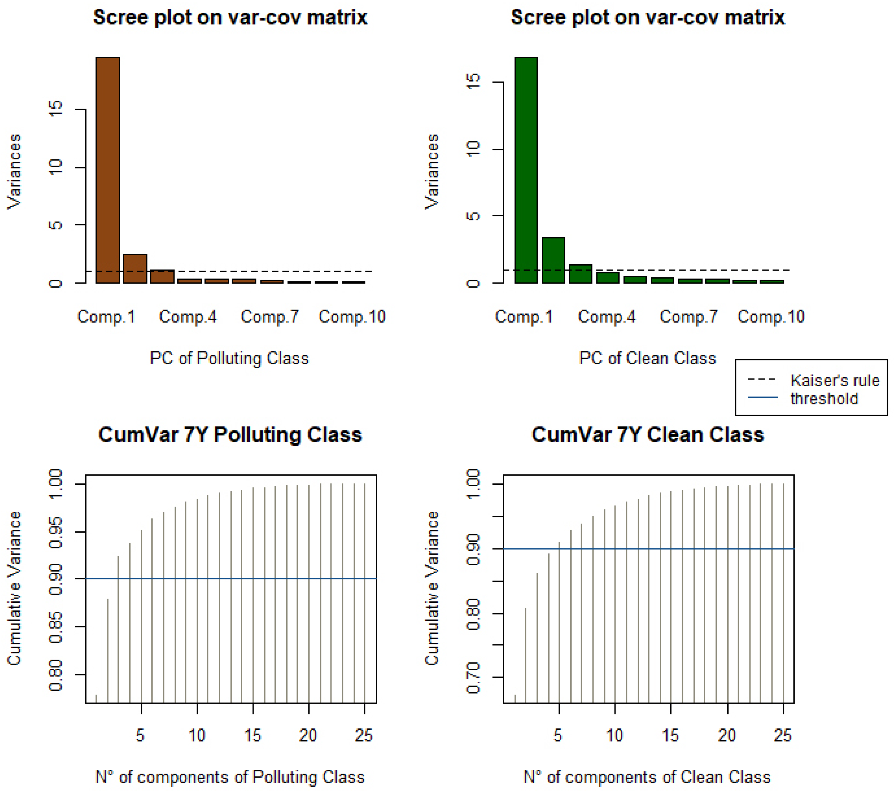
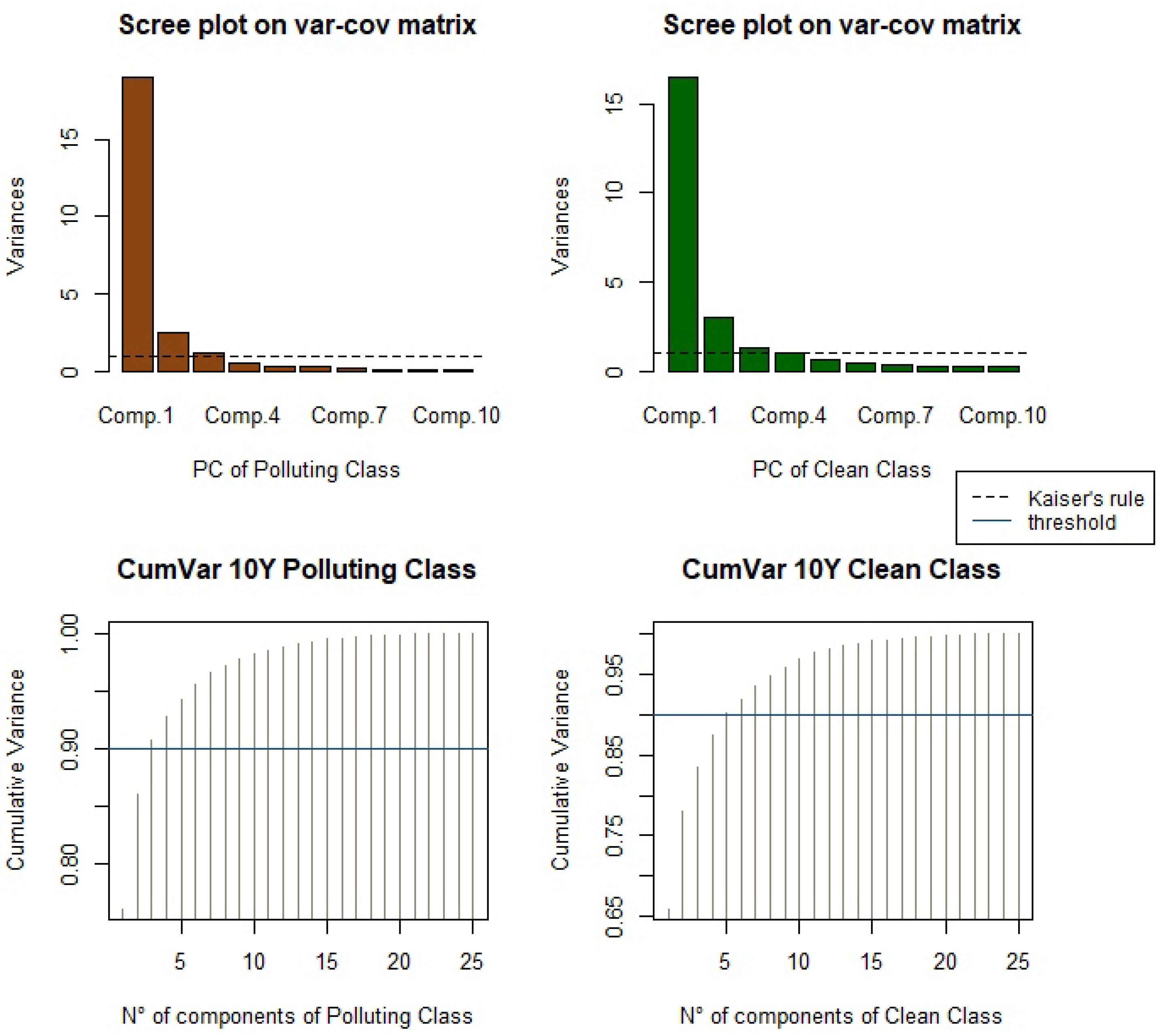
4.2. Preliminary Analysis through PCA

A preliminary analysis was conducted to further analyze the polluting and clean classes through a principal component analysis (PCA) with the goal of identifying the number of factors that drive the variability observed in the classes. PCA is a well-known method for dimension reduction while retaining a certain level of variability from the original data set.

The data set used in this section is the 5-year standardized CDS spread observations. The use of PCA on a standardized data set implies that the dimension-reduction approach has been explicitly applied to the correlation matrix of the initial data set to ensure that all variables are on the same scale and that those with more variability do not dominate the study. An issue when performing PCA concerns the number of principal components to consider. Some common criteria considered in the literature include the use of a scree plot paired with Kaiser’s rule2, or defining a high threshold for the explained cumulative variance of the principal components. In light of this, Figure 4 illustrates two distinct graphs for the polluting class, shown in brown on the left, and the clean class, shown in green on the right. The two methods are described here:

(i)

A scree plot (top), which illustrates the eigenvalue of each principal component, typically paired up with Kaiser’s rule, depicted by the straight black line. The eigenvectors represent the principal components of the data, and the corresponding eigenvalues indicate the amount of variance explained by each component.

(ii)

A histogram-like plot (bottom), which illustrates the cumulative variance explained by each principal component, given as the cumulative sum of the eigenvalues divided by the total sum of these eigenvalues. For this study, a cumulative variance explained by a threshold equal to 90%, indicated by the dark blue dashed line, was adopted.

The explained cumulative variance criteria were used for this section, with the scree plot paired up with Kaiser’s rule (the top graph), simply supporting the primary conclusions. Contrary to what we expected, the number of factors required for the cumulative variance in polluting and clean class actually differs, with the polluting class needing only three factors to explain a cumulative variance of 90% of the original data set, while the clean class required seven. Furthermore, as shown in

Table 3. Variances explained by the PC.

	Polluting Class		Clean Class
No.	Eigenvalue	Cumulative Variance (%)	Eigenvalue	Cumulative Variance (%)
1	18.74	74.98	14.87	59.50
2	2.96	86.83	3.48	73.41
3	0.97	90.71	1.57	79.70
4	-	-	0.98	83.63
5	-	-	0.89	87.20
6	-	-	0.67	89.87
7	-	-	0.61	92.30

, the first principal component of the polluting class already explains around 75% of the variance of the original data set, while the first principal component of the clean class only explains 60%. The same quantitative results for different tenors have been found, with the polluting class requiring fewer factors to explain a certain level of variability than the clean class; the results are provided in Appendix C. A possible explanation may be the fact that the components of the polluting class belong to more concentrated sectors (like Materials or Utility) compared to the constituents of the clean class, which are dispersed over a range of sectors.

4.3. Hypothesis Validation

We examine the relationship between the CR factor and CDS spread returns by attempting to validate some of proposed hypotheses in Blasberg et al.’s (2022) work. Contrary to the panel quantile regression employed by the authors, in this study, we performed quantile regression on time series data to comprehend the influence of the explanatory factors on the response variable based on the evolution of the data under consideration, which in this case correspond to the CDS spread returns. The baseline response variable, $s_t^m$, was constructed by assigning equal weights to all 56 components. As for the explanatory variables, only key firm-specific determinants of CDS spread returns were taken into account. Thus, the main equation considered is:

$$Q_{s_t^m}\left(\tau \right|x_t)={\alpha }_{\tau }+{\beta }_{\tau ,1}{r}_t+{\beta }_{\tau ,2}\Delta {\sigma }_t+{\beta }_{\tau ,3}\Delta {\mathrm{CR}}_t^m+{ϵ}_t,$$

(3)

where for the CDS issued on day t, firm-specific factors (made up by stock return $r_t$ and volatility $\Delta {\sigma }_t$) and the market-implied proxy for carbon risk exposure, $\Delta {\mathrm{CR}}_t^m$, are considered. The regression was performed for the median (considered as the benchmark) and the extremes of the distribution. In other words, the quantile regression was performed for the following percentiles in order to represent the influence of each explanatory variable on the extreme areas of the conditional distribution of CDS spread returns: $\tau \in \{0.01,0.05,0.1,0.5,0.9,0.95,0.99\}$. Given the percentiles considered, the relationship between CDS spread returns and the CR factor may be examined for firms that behave as the median of the conditional distribution, as well as those who overperform and underperform in terms of creditworthiness relative to the median. More specifically:

(i)

An increase in the CDS spread, which is for $\tau >0.5$, indicates a deterioration in a firm’s creditworthiness;

(ii)

A decrease in the CDS spread, which is for $\tau <0.5$, indicates an improvement in a firm’s creditworthiness;

(iii)

The median, $\tau =0.5$, corresponds to an unchanged CDS spread.

All analyses were carried out in R, with the quantreg package used to perform quantile regression, using the $rq$ function, which minimizes a weighted sum of absolute residuals that can be expressed as a linear programming problem. Lastly, standard error estimates of quantile regression coefficients were constructed using the non-parametric bootstrap method.

To validate the finding of Blasberg et al. (2022) regarding the positive relationship existing between the carbon risk factor and CDS spread returns, issuing firms were regrouped using the Bloomberg ESG Classification System (BECS) to isolate and assess the influence of the CR factor for each sector present in the sample, as shown in

Table 4. Coefficient estimates in a quantile regression model of the CR factor for 5-year CDS spreads for each sector considering the entire data set (upper part) and only the data of the calendar year 2022 (lower part).

Variable	$\mathit{\tau }=$ 0.01	$\mathit{\tau }=$ 0.05	$\mathit{\tau }=$ 0.1	$\mathit{\tau }=$ 0.5	$\mathit{\tau }=$ 0.9	$\mathit{\tau }=$ 0.95	$\mathit{\tau }=$ 0.99
Consumer Discretionary	0.80	3.68	3.45	1.92	0.42	−1.86	1.21
	(2.91)	(1.52)	(1.20)	(1.27)	(1.75)	(1.72)	(3.78)
Materials	11.85	5.08	4.87	3.93	2.36	3.28	0.33
	(15.41)	(2.15)	(1.21)	(0.93)	(1.86)	(2.65)	(10.96)
Industrial Products	−2.75	1.49	1.92	1.75	0.92	0.03	−3.92
	(5.96)	(3.00)	(1.73)	(1.10)	(1.61)	(1.95)	(4.85)
Utilities	9.76	5.15	3.97	4.44	3.05	3.21	1.17
	(5.44)	(1.69)	(1.68)	(1.09)	(1.39)	(1.56)	(2.35)
Energy	7.99	4.88	5.67	4.45	5.42	6.95	3.57
	(5.18)	(2.82)	(1.73)	(0.86)	(2.69)	(3.45)	(4.11)
Consumer Staples	4.21	3.32	3.67	3.11	3.21	3.18	−6.14
	(3.02)	(1.70)	(1.19)	(1.45)	(1.42)	(1.76)	(7.02)
Communications	2.56	1.47	1.33	1.56	−0.37	0.13	−4.70
	(4.53)	(2.14)	(1.42)	(0.78)	(1.35)	(1.96)	(7.34)
Healthcare	7.79	6.16	5.16	2.14	1.30	−0.49	6.29
	(3.74)	(2.20)	(1.78)	(1.00)	(2.70)	(3.60)	(6.92)
Technology	6.70	7.41	4.13	1.25	0.88	−1.56	−10.37
	(5.04)	(1.82)	(1.33)	(0.98)	(2.17)	(3.06)	(6.80)
Materials (2022)	15.63	11.05	10.14	6.18	2.79	0.31	−3.37
	(31.16)	(3.75)	(2.60)	(1.39)	(3.26)	(2.61)	(31.94)
Utilities (2022)	15.94	13.30	12.55	8.62	2.80	2.36	−0.94
	(6.66)	(3.65)	(2.54)	(1.21)	(2.67)	(3.23)	(4.39)
Energy (2022)	16.50	16.06	12.77	7.32	9.72	56.16	5.15
	(11.83)	(4.32)	(3.56)	(1.72)	(5.31)	(6.61)	(5.76)

, which refers to 5-year tenors3 with coefficient estimates scaled by factor of $1\times {10}^3$. Only three sectors, Consumer Discretionary, Industrial Products and Consumer Staples, are present in both polluting and clean classes. Moreover, in the polluting class, carbon-intensive sectors such as Materials, Energy and Utilities exhibit higher coefficient estimates than the rest of the sectors. Similarly, Healthcare and Technology have significant coefficient values for the clean class. According to the recent literature, Blasberg et al. (2022); Zhang et al. (2023), carbon risk significantly influences firms’ valuations. This suggests that carbon-intensive sectors, which make up the majority of the polluting class, may face increased credit risk due to higher values of coefficient estimates for the CR factor. Businesses in less carbon-intensive sectors, in comparison, are seen as better equipped to provide the necessary innovation and technological advances for the transition to a low-carbon economy. As a result, their coefficient estimates for the CR factor are generally lower, implying that enterprises in this sector are less affected by carbon risk. Given that 2022 was characterized by the Russo–Ukrainian War, the last rows of Table 4 display the coefficient estimates for selected sectors of the polluting class for 2022. In particular, only sectors with the highest coefficient estimates are provided, which corresponded to the carbon-intensive industries significantly affected by the conflict, namely Materials, Utilities and Energy.

Another hypothesis in Blasberg et al. (2022) asserts a positive relationship between the term structure of carbon risk and CDS spread slopes. This will be investigated by looking at how changes in the expected realization of carbon risk affect the term structure of a firm’s credit risk. In light of this, the CDS spread term structure has been considered to establish the shape of the default probability across various time periods. The changes in the CDS slope (response variable) were computed as the difference between two CDS spreads of differing maturities, $m\ne n$, as $CD{S}_t^{mn}=CD{S}_t^m-CD{S}_t^m$. In formulas, it reads:

$$\Delta {\mathrm{CDSSlope}}_t^{mn}={\mathrm{CDSSlope}}_t^{mn}-{\mathrm{CDSSlope}}_{t-1}^{mn}.$$

(4)

Figure 5 describes the realizations of the Euribor 12-month rates, obtained from FactSet, for the sample period, which proxies the variable that we call the interest rate (IR). Starting at levels below zero, the overnight interbank rate increased on July 2022, marking its first increase in more than ten years, as the European Central Bank (ECB) addressed eurozone inflation in response to an upsurge in food and energy prices. This inflation was primarily triggered by more expensive energy as a result of the COVID-19 pandemic, which was aggravated by the Russo–Ukrainian conflict. In particular, changes in the Euribor 12-month rates, $\Delta {\mathrm{IR}}_t$, were taken into account. According to Blasberg et al. (2022), an increase in the reference interest rate decreases the default probability, leading to CDS spread declines. In short, we assume there is an inverse relationship between the CDS spread slope and the interest rate factor. In addition, the market’s outlook on future interest rates was included, as represented by the fluctuations in the difference between the Euribor 3-month rates and Euribor 12-month rates, $\Delta {\mathrm{Term}}_t$ Blasberg et al. (2022); Han and Zhou (2015). Consequent fluctuations in this factor boost the default probability, prompting CDS spreads to increase. In short, there is a direct relationship between the slope of the CDS spreads and the term factor. The only firm-specific variable in this section is the change in historical stock volatility, $\Delta {\sigma }_t$. Finally, the slope of the CR factor is determined as ${\mathrm{CRSlope}}_t^{mn}={\mathrm{CR}}_t^m-{\mathrm{CR}}_t^n$, with $m>n$. As a result, the model used to validate this final hypothesis reads as follows:

$$Q_{\Delta {\mathrm{CDSSlope}}_t^{mn}}\left(\tau \right|x_t)={\alpha }_{\tau }+{\beta }_{\tau ,1}\Delta {\sigma }_t+{\beta }_{\tau ,2}\Delta {\mathrm{IR}}_t+{\beta }_{\tau ,3}\Delta {\mathrm{Term}}_t+{\beta }_{\tau ,4}\Delta {\mathrm{CRSlope}}_t^{mn}+{ϵ}_t.$$

Table 5. Coefficient estimates of the CR slope factor.

Variable	$\mathit{\tau }=$ 0.01	$\mathit{\tau }=$ 0.05	$\mathit{\tau }=$ 0.1	$\mathit{\tau }=$ 0.5	$\mathit{\tau }=$ 0.9	$\mathit{\tau }=$ 0.95	$\mathit{\tau }=$ 0.99
5Y-1Y
$\Delta {\sigma }_t$	−14.76	−2.11	−1.09	−0.10	0.45	1.95	−6.10
	(11.37)	(2.05)	(0.70)	(0.31)	(1.00)	(2.06)	(10.88)
$\Delta {\mathrm{IR}}_t$	−8.19	−7.91	−2.59	−0.11	−2.00	−0.55	−11.34
	(25.21)	(5.05)	(2.85)	(0.74)	(1.80)	(2.48)	(15.32)
$\Delta {\mathrm{Term}}_t$	−16.69	6.91	1.81	−0.42	1.06	−0.10	−4.43
	(26.09)	(5.19)	(2.29)	(0.70)	(1.61)	(3.20)	(18.17)
$\Delta \mathrm{CR}{\mathrm{Slope}}_t$	17.63	1.46	−0.05	−0.07	0.10	−3.91	15.87
	(15.07)	(2.39)	(1.01)	(0.46)	(1.28)	(2.68)	(8.84)
10Y−1Y
$\Delta {\sigma }_t$	−22.42	−3.19	−2.71	−1.04	0.61	1.58	4.89
	(10.73)	(1.52)	(0.63)	(0.93)	(0.80)	(1.66)	(8.29)
$\Delta {\mathrm{IR}}_t$	−67.92	−4.03	−5.32	3.01	2.74	1.77	−0.58
	(49.91)	(8.00)	(3.90)	(2.65)	(1.08)	(2.82)	(12.10)
$\Delta {\mathrm{Term}}_t$	43.50	1.89	1.07	−1.44	−0.92	−2.73	−6.35
	(21.02)	(3.31)	(1.13)	(1.02)	(0.67)	(1.86)	(10.75)
$\Delta \mathrm{CR}{\mathrm{Slope}}_t$	−18.38	−2.86	−0.36	−0.93	−1.87	−3.19	−6.75
	(17.18)	(2.89)	(1.33)	(0.53)	(0.74)	(1.55)	(10.71)

reports the findings for the 5Y-1Y slope and the 10Y-1Y CR slope scaled by a factor of $1\times {10}^3$, with the short-term effect, referring to the following four years, represented by the 5Y-1Y slope and the long-term effect, referring to the following nine years, represented by the 10Y-1Y slope. Essentially, a positive (negative) CR slope coefficient indicates tighter (looser) carbon regulations and a heightened (lowered) exposure to the transition risk for the longer term, as discussed in Blasberg et al. (2022). Interestingly, the coefficient estimates for 5Y-1Y for $\Delta {\mathrm{IR}}_t$ establish a negative relationship between the CDS spread slope and the changes in risk-free interest rates, in comparison to the assumption stated above. The positive relationship between the response variable and the explanatory factor $\Delta {\mathrm{Term}}_t$ is not evident in the sample period considered. The massive spike in interest rates in the European market in recent years might be a plausible cause for this. In particular, for the shorter tenor, the coefficient estimates for the CR slope factor have values that vary along zero for certain quantiles and are extreme in others. Additionally, the coefficient estimates seem to be significantly negative over the longer term. According to this result, the market anticipates that changes in the European carbon regulation framework to be less strict and more flexible over the course of the next four years, but notably over the course of the next nine years. This highly contradicts Blasberg et al. (2022)’s assumption that the market interprets carbon risk as a short-to-medium-term risk, as central banks anticipate. Nonetheless, these unexpected findings might just be a result of the current market conditions, which are being driven by rising interest rates, as seen in Figure 5, in an attempt to battle inflation.

Finally,

Table 6. Coefficient estimates of the CR slope factor over the years.

Variable	$\mathit{\tau }=$ 0.01	$\mathit{\tau }=$ 0.05	$\mathit{\tau }=$ 0.1	$\mathit{\tau }=$ 0.5	$\mathit{\tau }=$ 0.9	$\mathit{\tau }=$ 0.95	$\mathit{\tau }=$ 0.99
2020
$\Delta$ CR Slope 5Y-1Y	7.01	−0.74	0.90	−0.60	2.46	6.54	27.24
	(21.52)	(9.51)	(1.60)	(1.13)	(1.94)	(4.93)	(11.22)
$\Delta$ CR Slope 10Y-1Y	−20.89	−1.84	−0.48	1.73	−1.86	−0.72	−0.27
	(16.81)	(8.36)	(3.36)	(1.68)	(1.62)	(1.86)	(11.70)
2021
$\Delta$ CR Slope 5Y-1Y	−21.11	−4.67	−2.93	−1.15	−2.63	−0.44	−8.90
	(14.51)	(6.81)	(2.18)	(0.67)	(2.01)	(7.60)	(12.37)
$\Delta$ CR Slope 10Y-1Y	−6.56	−4.20	−0.91	−0.29	0.24	1.19	16.72
	(17.13)	(6.93)	(3.23)	(1.00)	(2.53)	(5.27)	(9.81)
2022
$\Delta$ CR Slope 5Y-1Y	41.73	−1.72	0.13	0.21	−2.42	−7.23	−14.52
	(20.21)	(5.00)	(1.23)	(0.55)	(2.11)	(2.68)	(6.60)
$\Delta$ CR Slope 10Y-1Y	0.49	−8.14	−3.23	−2.57	−3.53	−8.21	+17.52
	(29.82)	(6.82)	(2.74)	(1.09)	(1.89)	(4.94)	(10.91)
2023
$\Delta$ CR Slope 5Y-1Y	−15.59	14.21	9.07	3.13	−1.65	−1.16	23.28
	(33.49)	(9.97)	(7.14)	(3.33)	(8.73)	(17.41)	(20.91)
$\Delta$ CR Slope 10Y-1Y	−15.81	6.62	2.08	−0.11	−1.95	−1.99	11.51
	(10.49)	(6.41)	(4.14)	(2.70)	(4.25)	(6.80)	(12.20)

shows the coefficient estimates for the CR slope component for each year of the data set scaled by a factor of $1\times {10}^3$. The coefficient estimates for 2020 and 2021 are ambiguous and unclear due to shifting values along zero for both the short-to-medium and medium-to-long tenor, mirroring the findings for the whole sample period. This might be attributable to the steady trend in the CR factor along with risk-free interest rates that are still below zero, as shown in Figure 5. Following this, 2022, which is when the interest rate hikes occurred, was also distinguished by irregular coefficient estimates above zero. Finally, the results for the first half of 2023 are more aligned with Blasberg et al. (2022)’s findings, with greater coefficient estimates for the shorter term than for the longer term, which are always characterized by certain negative coefficient values for specific quantiles. Ultimately, the differing time periods investigated for this study compared to Blasberg et al. (2022) led to different results, with recent years marked by worrisome geopolitical and macroeconomic events. Nevertheless, the overall impact of carbon risk on firm creditworthiness continues to persist; hence, the ever-growing sustainable-aware market should not exclude this market-implied forward-looking component in their analysis.

5. Conclusions

This paper investigates the influence of the carbon risk factor on firms’ credit risk. The green and brown constituents were first studied through a PCA analysis, which suggested that a lower number of factors is required in order to reproduce a certain level of variability in the polluting class compared to the number of driving factors in the clean class. Then, several quantile regressions were carried out to validate the hypotheses proposed by Blasberg et al. (2022). In particular, we find a positive relationship between the exposure to carbon risk and the cost of default protection, with the impact being more pronounced in the extreme quantiles. This impact varies by company sector, with carbon-intensive sectors such as Materials, Energy and Utilities sectors having the largest estimated coefficients. The impact was substantially higher during the Russo–Ukrainian conflict in 2022, demonstrating how the markets have demanded more default protection for firms in these sectors following the conflict’s widespread repercussions throughout the European continent. Finally, further quantile regression models were considered by including the change in the interest rate as a control variable. Interestingly, the results suggest that the market anticipates changes in the European carbon regulation framework to be more flexible over the course of the next four years, but their effect should be notable over the course of the next nine years.

References

1. Bachelet, Maria J., Leonardo Becchetti, and Stefano Manfredonia. 2019. The green bonds premium puzzle: The role of issuer characteristics and third-party verification. Sustainability 11: 1098. [Google Scholar] [CrossRef]
2. Benz, Lukas, Stefan Paulus, Julia Scherer, Julia Syryca, and Stefan Trück. 2021. Investors’ carbon risk exposure and their potential for shareholder engagement. Business Strategy and the Environment 30: 282–301. [Google Scholar] [CrossRef]
3. Blasberg, Alexander, Ruediger Kiesel, and Luca Taschini. 2022. Carbon Default Swap-Disentangling the Exposure to Carbon Risk through CDS. CESifo Working Paper. Munich: CESifo. [Google Scholar]
4. Bolton, Patrick, and Marcin Kacperczyk. 2020. Do Investors Care about Carbon Risk? NBER Working Paper Series; Cambridge, MA: NBER. [Google Scholar]
5. Bro, Rasmus, and Age K. Smilde. 2014. Principal component analysis. Analytical Methods 6: 2812–31. [Google Scholar] [CrossRef]
6. Carbone, Sante, Margherita Giuzio, Sujit Kapadia, Johannes Krämer, Kwn Nyholm, and Katia Vozian. 2021. The Low-Carbon Transition, Climate Commitments and Firm Credit Risk. Frankfurt: European Central Bank. [Google Scholar]
7. Cheema-Fox, Alexander, Bridger LaPerla, George Serafeim, David Turkington, and Hui Wang. 2021. Decarbonizing Everything. Financial Analysts Journal 77: 93–108. [Google Scholar] [CrossRef]
8. European Central Bank. 2022. ECB Takes Further Steps to Incorporate Climate Change into Its Monetary Policy Operations. Frankfurt: ECB. [Google Scholar]
9. Flammer, Caroline, Michael Toffel, and Kala Viswanathan. 2021. Shareholder activism and firms’ voluntary disclosure of climate change risks. Strategic Management Journal 42: 1850–79. [Google Scholar] [CrossRef]
10. Galil, Koresh, Offer Mashe Shapir, Dan Amiram, and Uri Ben-Zion. 2014. The determinants of CDS spreads. Journal of Banking and Finance 41: 271–82. [Google Scholar] [CrossRef]
11. Hachenberg, Britta, and Dirk Schiereck. 2018. Are green bonds priced differently from conventional bonds? Journal of Asset Management 19: 371–83. [Google Scholar] [CrossRef]
12. Han, Bing, and Yi Zhou. 2015. Understanding the term structure of credit default swap spreads. Journal of Empirical Finance 31: 18–35. [Google Scholar] [CrossRef]
13. Jung, Juhyun, Kathleen Herbohn, and Peter Clarkson. 2018. Carbon risk, carbon risk awareness and the cost of debt financing. Journal of Business Ethics 150: 1151–71. [Google Scholar] [CrossRef]
14. Kleimeier, Stefanie, and Michael Viehs. 2021. Pricing carbon risk: Investor preferences or risk mitigation? Economics Letters 205: 109936. [Google Scholar] [CrossRef]
15. Koenker, Roger, and Gilbert Bassett. 1978. Regression Quantiles. Econometrica 46: 33–50. [Google Scholar] [CrossRef]
16. Mercuri, Lorenzo, Andrea Perchiazzo, and Edit Rroji. 2023. Investigating Short-Term Dynamics in Green Bond Markets. arXiv arXiv:2308.12179. [Google Scholar]
17. Merton, Robert. 1974. On the Pricing of Corporate Debt: The Risk Structure of Interest Rates. The Journal of Finance 29: 449–70. [Google Scholar]
18. Nguyen, Justin, and Hieu Phan. 2020. Carbon risk and corporate capital structure. Journal of Corporate Finance 64: 101713. [Google Scholar] [CrossRef]
19. Reboredo, Juan Carlos. 2018. Green bond and financial markets: Co-movement, diversification and price spillover effects. Energy Economics 74: 38–50. [Google Scholar] [CrossRef]
20. Sohag, Kazi, M. Kabir Hassan, Stepan Bakhteyev, and Oleg Mariev. 2023. Do green and dirty investments hedge each other? Energy Economics 120: 106573. [Google Scholar] [CrossRef]
21. Zhang, Yuqi, Yaorong Liu, and Haisen Wang. 2023. How credit default swap market measures carbon risk. Environmental Science and Pollution Research 30: 82696–716. [Google Scholar] [CrossRef] [PubMed]
Figure 1. Evolution of weighted averages of (log) CDS spreads in the polluting (brown line) and in the green class (green line) for all maturities.
Risks 12 00016 g001
Figure 2. Relative changes in CDS spreads for all maturities.
Risks 12 00016 g002
Figure 3. Histogram of CDS spreads for all maturities. The blue curve is the fitted normal distribution.
Risks 12 00016 g003
Figure 4. PCA results for 5-year CDS spreads.
Risks 12 00016 g004
Figure 5. Evolution of Euribor 12-month rates.
Risks 12 00016 g005