Article

Cyber Risk Contagion

Department of Economics and Management, University of Pavia, Via San Felice 5, 27100 Pavia, Italy
*
Author to whom correspondence should be addressed.
These authors contributed equally to this work.
Risks 2023, 11(9), 165; https://doi.org/10.3390/risks11090165
Submission received: 11 August 2023 / Revised: 11 September 2023 / Accepted: 15 September 2023 / Published: 19 September 2023

Abstract

:
Financial technologies (fintechs) are continuously expanding, across different markets and financial services. While financial technologies bring many opportunities, such as reduced costs and extended inclusion, they also bring risks, among which include cyber risks, that are difficult to measure. One of the difficulties that arise in the measurement of cyber risks is the interdependence among cyber losses, a problem that has not yet been solved. To fill the gap, this paper proposes a multivariate model for cyber risks, based on their observed time series of counts. The time-varying intensity parameter of the model determines the probability that a cyber attack occurs, and its specification takes not only time but also sectorial interdependence into account. The effectiveness of the proposed model is demonstrated by means of a real cyber loss dataset, in which there exists time and sectorial dependence among different events.

1. Introduction

The Financial Stability Board defines financial technologies as “technologically enabled financial innovations that could result in new business models, applications, processes, or products with an associated material effect on financial markets and institutions and on the provision of financial services”. While financial technologies can bring important opportunities, such as improved user interface, better financial inclusion, and lower costs, they can also carry new risks, including cyber risks (see, for example, Kopp et al. 2017).
To improve the adoption of financial technologies, a framework for cyber risk management becomes necessary. In the last few years, the number of cyber attacks on information technology (IT) systems has surged. For example, 1460 cyber attacks have occurred in 2018 and 1127 attacks occurred in 2017, against 1050 in 2016, 1012 in 2015 and 873 in 2014, with a growth of about 30 % between 2014 and 2017. The trend in from 2020 onwards follows a similar path, especially after the COVID-19 pandemic, although final figures are not yet available.
In line with the growing relevance of the problem, the extant literature has recognized the need to measure cyber risks (see, for example, Kure et al. 2021; Mazzoccoli and Naldi 2021; Paté-Cornell et al. 2017; Facchinetti et al. 2020; Ruan 2019; Florackis et al. 2023; Eling and Wirfs 2019; Eling 2020; Giudici and Raffinetti 2021; Chande and Yanchus 2019).
Cyber risk measurement models suffer from lack of data, typically for non-disclosure reasons. To solve this problem, cyber loss data can be modeled using ordinal variables, following the literature on operational risk measurement (see, for example, Aldasoro et al. 2022; Chernobai et al. 2019; Curti et al. 2022; Cohen et al. 2019; Giudici and Raffinetti 2021 and the references therein).
Cyber risks are strictly related to operational risks and, therefore, may share similar loss models, in the univariate case (see, for example, Aldasoro et al. 2022). However, different from operational risks, cyber risks have a strong multivariate dependence, which arises from the interdependence between cyber events. Interdependence may arise, in particular, from the fact that cyber attacks often have multiple targets, and that most fintech activities employ cloud computing. The presence of interdependence can lead to a systemic risk similar to that analyzed in financial markets, which has attracted the attention of researchers and regulatory authorities (see, for example, Diebold and Yılmaz 2014; Tobias and Brunnermeier 2016; Escribano and Maggi 2019; Lando and Nielsen 2010; Agosto et al. 2016, 2020; Ahelegbey et al. 2016; Billio et al. 2012; Aldasoro et al. 2022; Giudici et al. 2019; Danielsson and Macrae 2019).
While the literature on systemic risks arising from financial markets is quite abundant, that on systemic risk arising from cyber losses is not yet available. We propose to fill this gap with the present paper, which aims to contribute to cyber risk measurement by means of a methodology able to capture interdependencies among cyber losses.
More specifically, the contribution of this paper is to develop a contagion model for cyber risks that is based on a multivariate model for count time series of cyber risk events. The model was introduced by Agosto (2022) for credit markets and has a score-driven specification: the time-varying intensity parameter determining the probability that an extreme market event occurs follows the specification of generalized autoregressive score (GAS) models, also known as dynamic conditional score models (Creal et al. 2013; Harvey 2013). In the GAS framework, time-varying parameters depend on their lagged values and on the scaled score of the conditional observation density. GAS models belong to the class of observation-driven models and are found to perform comparably to parameter-driven models in terms of predictive accuracy. From a computational point of view, they can be easily estimated through maximum likelihood optimization.
We apply the model to the daily count of cyber events in different economic sectors, from 2018 to 2021, and find significant time dependence, along with some cross-sector effects.
The next table summarizes our contribution with respect to the related literature discussed above.

2. Materials and Methods

A well-known distribution for non-negative integer variables is the negative binomial, which generalizes the Poisson distribution. The negative binomial distribution is derived from the Poisson-gamma mixture and is characterized by a location parameter μ —also defined as the intensity of the count process—and a dispersion parameter α . The higher α , the higher the overdispersion in the data. Indeed, when α = 0 , the negative binomial distribution reduces to the Poisson one, where the variance is equal to the mean. The negative binomial distribution is known to be particularly suitable for modeling the count time series of rare events, such as the number of cyber attacks analyzed in this paper.
Following Agosto (2022), we assume that the observations in each count time series of cyber events i follow a negative binomial distribution with a time-varying location parameter μ i t > 0 and a static dispersion parameter α i 0 :
X i t N B ( μ i t , α i )
First, we reparametrize the location parameter through an exponential link: f t = log ( μ t ) . This is a common choice in the specification of generalized linear models, as it ensures strict positivity of the time-varying parameter without imposing restrictions on the coefficients. Then, to model the time-varying location parameters f t = log ( μ t ) , we use a generalized autoregressive score (GAS) specification (Creal et al. 2013; Harvey 2013). In the general GAS specification, the dynamics of filtered parameters f t + 1 = ( f 1 , , f t ) are captured by an autoregressive term and by the scaled score (gradient) of the conditional observation density through the recursions
f t + 1 = C + B f t + A S ( f t ) ( x t , f t )
where f t = ( f 1 t , , f k t ) is the vector of time-varying parameters, C = ( c 1 , , c k ) are the constant parameters, B = d i a g ( b 1 , , b k ) is the k × k diagonal matrix of autoregressive parameters, A is the k × k matrix of coefficients associated to the scaled score and S ( f t ) is a scaling function for the score ( x t , f t ) . Moreover, we assume
A = d i a g ( e ) + γ δ
where e, γ , and δ R k are column vectors. In addition, to identify the model and estimate the values of γ and δ , following Heinen and Rengifo (2007), we impose δ k = 1 i = 1 k 1 δ i .
The score ( x t , f t ) is a k × 1 vector corresponding to the first derivative of the negative binomial log-likelihood function. It can easily be shown that it can be calculated through the following formula:
( x t , f t ) = x t exp ( f t ) α exp ( f t ) + 1
Without loss of generality, we use a unit scaling, that is, we assume S ( f t ) = I k .
In the context of our cyber risk application, the coefficients in the A matrix express in-sector and cross-sector dependence through the score. Indeed, as it can be seen from Formula (4), the score is calculated as the scaled difference between the observed and expected number of events (i.e., the shock) at the previous time. Thus, the A coefficients determine the impact of unexpected cyber losses that occurred in t 1 on the expected cyber losses in t in the same sector (diagonal effects) and in other sectors (off-diagonal effects). Formulation (3) gives further insight into the interpretation of parameters: e measures the own effect of shock events in sector i, while the γ and δ vectors act as multipliers of the off-diagonal elements of A. The B coefficients express, instead, the dependence of the expected number of cyber losses on past expectations, while the C constant parameters determine the unconditional and long-term mean of the number of events.
The model coefficients can be estimated through maximum likelihood optimization (see Agosto (2022) for details).

3. Results

3.1. Data

We apply our modeling approach to the daily cyber attack data collected by an international data provider in an agnostic and independent manner, which essentially involves transforming each news of cyber attacks into a severity scale that goes from “low” to “high” values. The data, which can be publicly visualized at www.hackmanac.com (accessed on 28 February 2023).
The data have already been analyzed by means of rank regression models in Giudici and Raffinetti (2021). Here, we extend the work, taking into account time and sectorial dependence.
For each day in the analyzed time period, we count the number of cyber attacks in each of the following sectors: education, government, healthcare, financial, information and communication technology (ICT), and trade. We consider only high-severity events, corresponding to “high” or “critical” losses. Thus, we end up with six count time series of extreme events.
We remark that all the considered series show a high frequency of zeros and are overdispersed, i.e., their variance is higher than the mean. These features motivate the use of count data models for rare events, allowing for possible zero-inflation and overdispersion.

3.2. Empirical Findings

We now present the results of fitting the negative binomial score-driven model presented in Section 2 to the time series of cyber attacks to different economic sectors in the 2018–2021 period (see Section 3.1). By letting the α coefficients equal to those estimated at the univariate level and maximizing the log-likelihood, we estimate the parameters entering the score-driven dynamics and obtain predictions for the counts.
The coefficients entering the score-driven dynamics (2)—estimated through likelihood maximization—are shown in Table 1 and Table 2. In particular, Table 1 reports the c constant parameters entering the C matrix in Formula (2), as well as the b diagonal entries of the B matrix, which express the dependence of each count time series on its previous values. Table 2 shows, instead, the coefficients entering the A matrix in Formula (2), expressing the cross-sector impacts of the cyber attack counts.
The values in Table 1 indicate, along with significant constant parameters, the presence of significant in-sector time dependence (expressed by the b autoregressive coefficients) for all sectors and, particularly, for the education one. This is in line with the observation that, during the COVID-19 period, on-line educational services have substantially increased and, along with them, cyber attacks to educational institutions.
On the other hand, Table 2 captures the sectorial dependence among cyber attacks. In particular, coefficients in row i in Table 2 express the impact that shocks to the number of cyber attacks in other sectors (along the columns) have on sector i, while coefficients in column j measure the extent to which cyber attacks in sector j affect the others (along the rows). The value of the off-diagonal elements, capturing cross-sector dependence, is determined by the γ and δ parameters entering specification (3). Based on this interpretation of coefficients, which arises from our model specification, the row sum of non-diagonal coefficients in the A matrix for a given sector can be considered a measure of its in-strength centrality, while the column sum of non-diagonal coefficients can be read as a measure of the sector’s out-strength centrality.
The diagonal elements of the A matrix can be instead interpreted as in-sector channels of contagion, that is, the impact of shocks to the number of cyber attacks in a sector on the expected number of cyber attacks in the same sector. Their value is determined by the estimated e parameters, according to (3).
Based on our results, the sector that affects others most strongly turns out to be ICT, followed by government, both particularly impacting the educational sector. In fact, the columns corresponding to the ICT and the government sectors in Table 2, containing the coefficients that express the impact of cyber attack counts among ICT and government companies to cyber attacks counts in other sectors, show two significant values (marked in bold) in the education row, meaning that the latter sector is significantly impacted by the ICT (with higher magnitude) and government sectors in terms of cyber risk. The result is in line with the intuition that the ICT sector, being more dependent on technology, is also more subject to attacks, whereas the government sector, being strategic for a country, plays a rather central role. Looking instead at “in-strength” centrality, the sector most impacted by cyber attacks in other sectors is the educational one. Indeed, the row corresponding to the educational sector in Table 2, which reports the coefficients associated with the impact of other sectors’ counts on educational institutions, is the only one that shows two significant non-diagonal coefficients, corresponding to the effect of the government and ICT sectors. This is in line with the intuition that the educational sector is often among the most open to innovations and the least protected. The educational sector is also the one that shows the highest in-sector dependence, as it shows the highest diagonal coefficient in the A matrix.
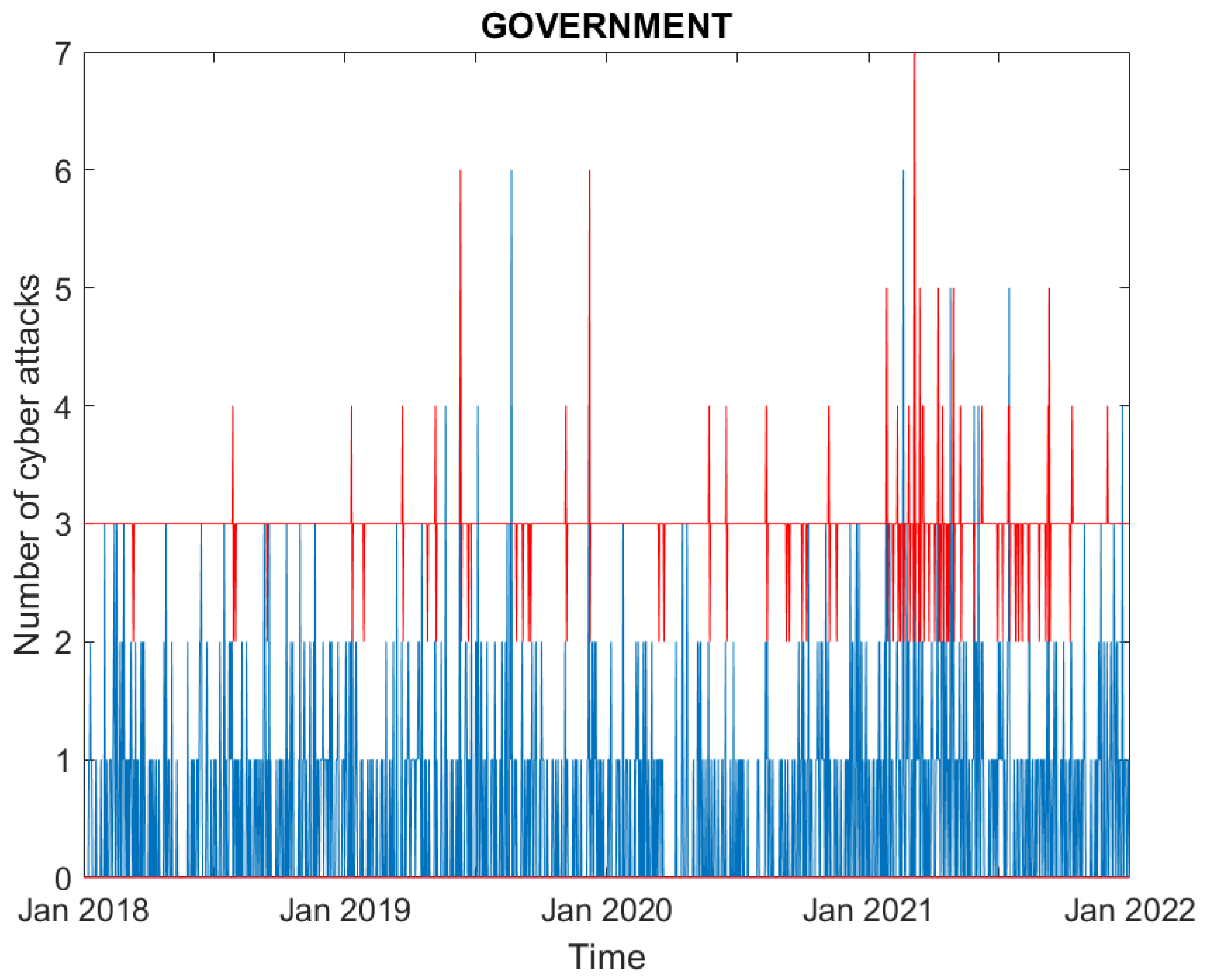
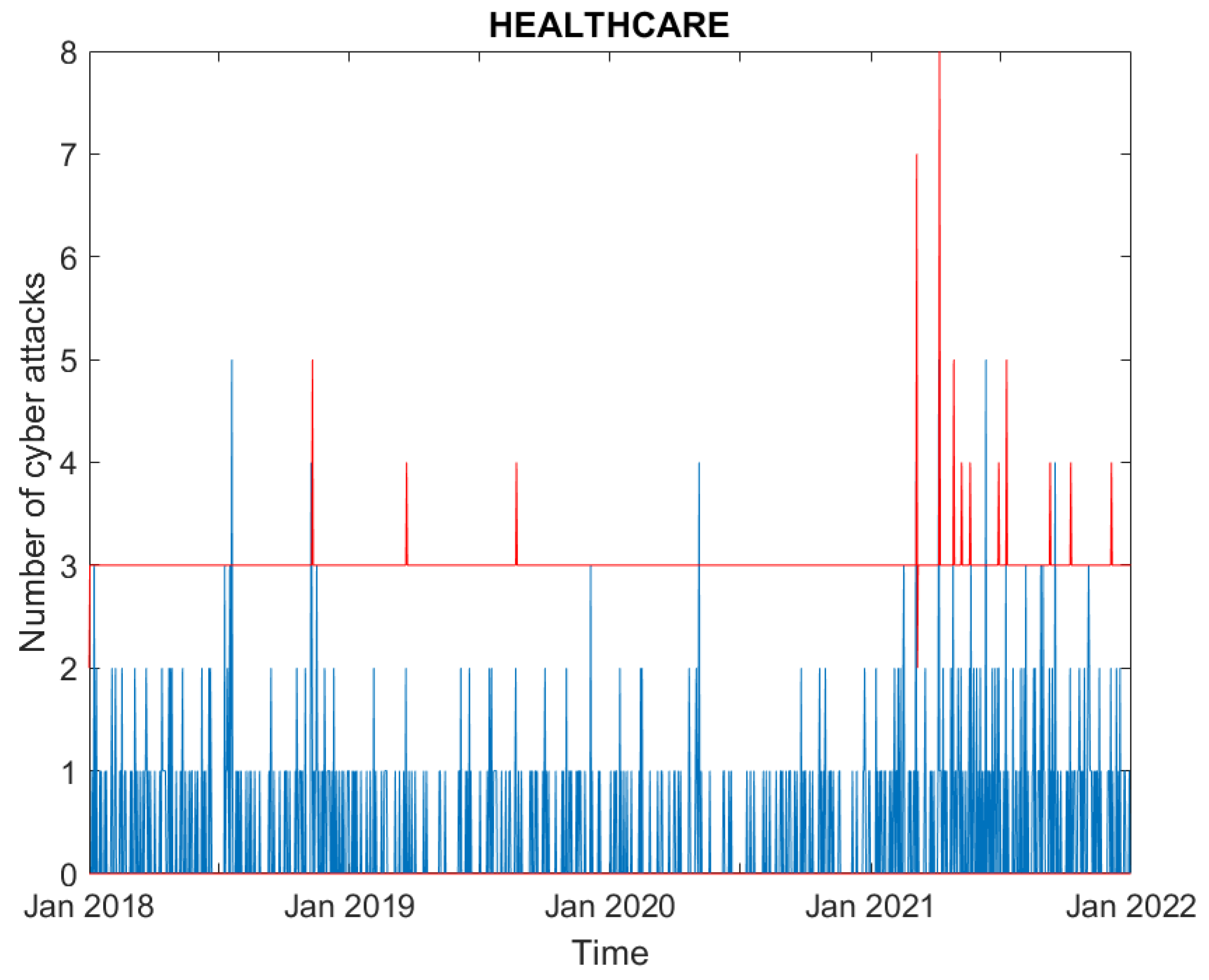
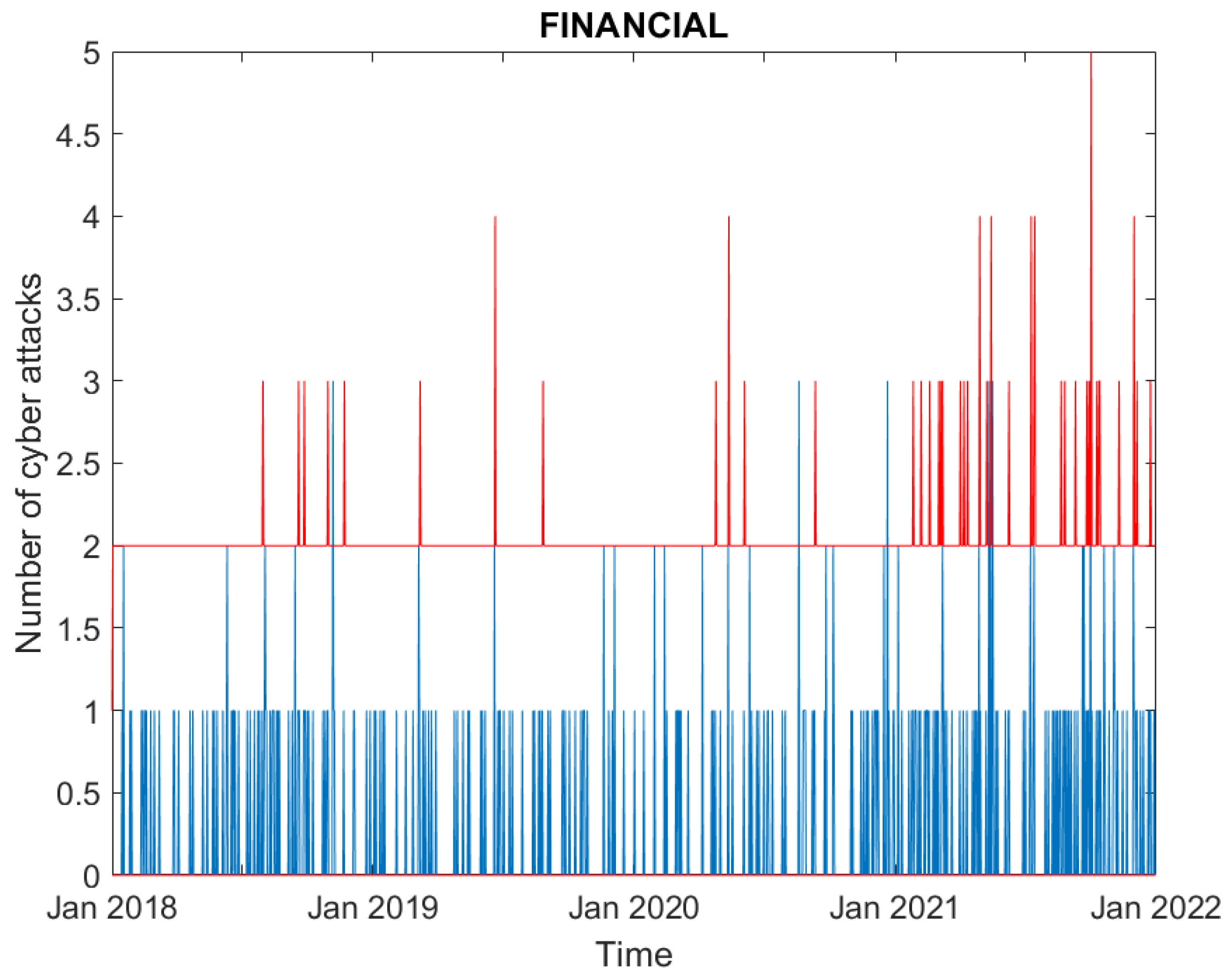
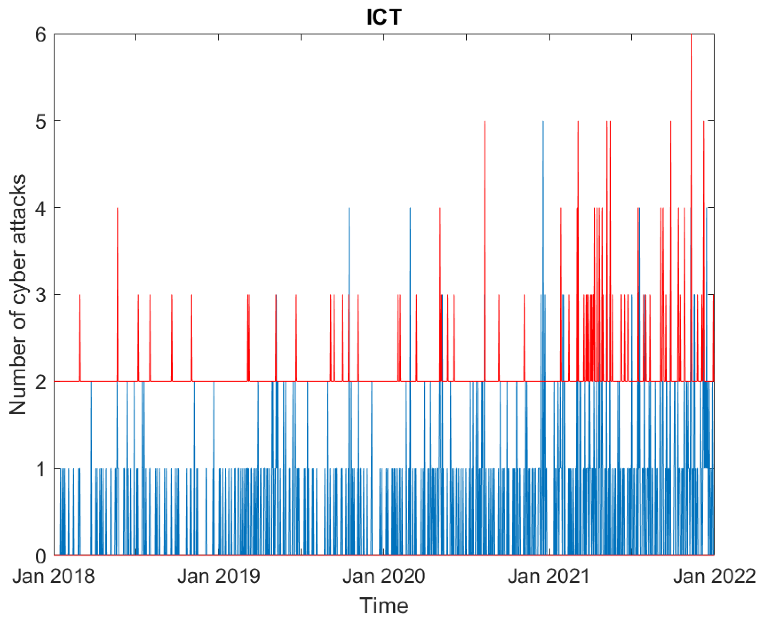
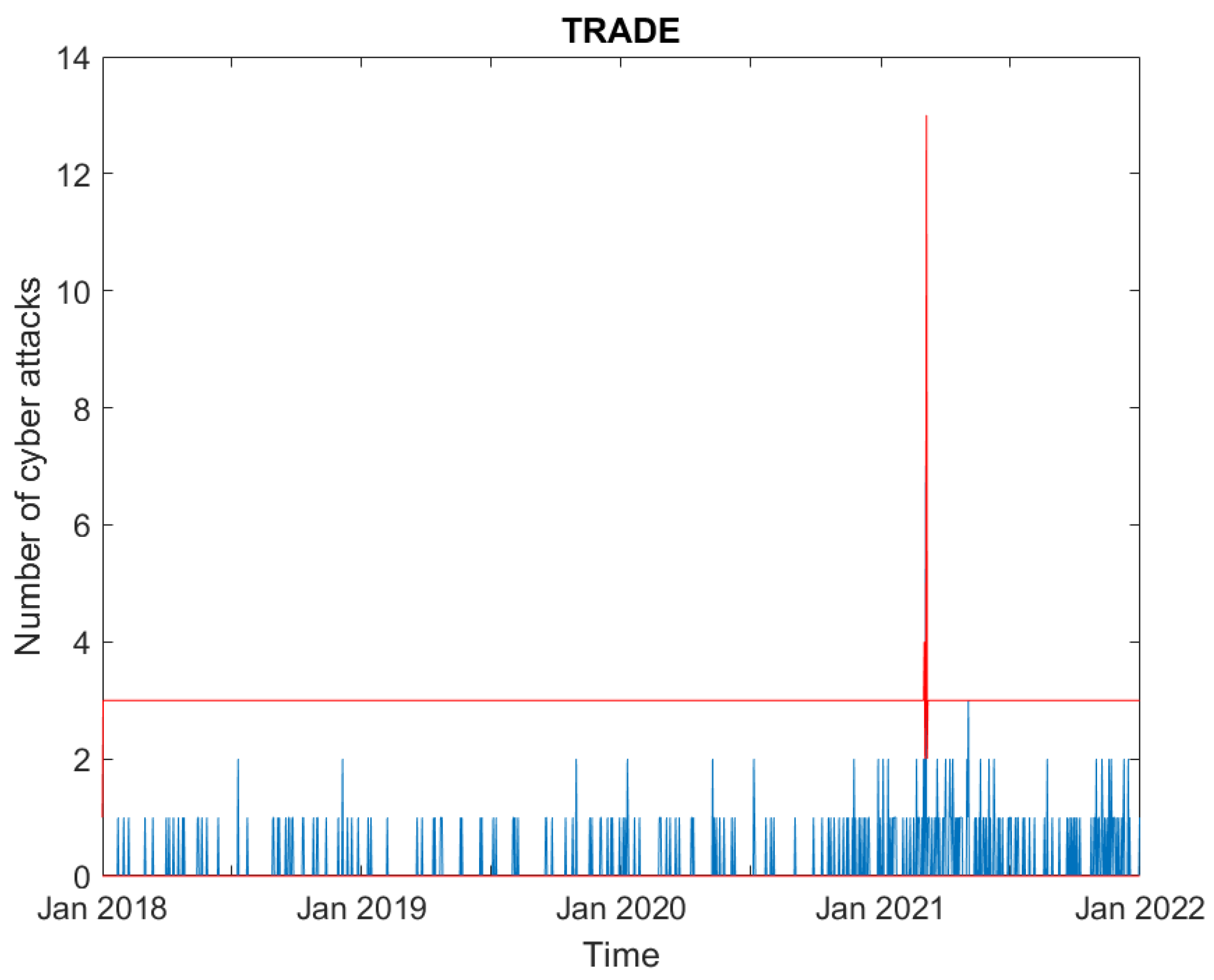
We now evaluate the performance of the proposed model by comparing the observed and fitted counts. In particular, Figure 1, Figure 2, Figure 3, Figure 4, Figure 5 and Figure 6 compare, for each time series, the observed counts against the 95% confidence bands for the fitted ones, calculated by applying the negative binomial distribution function with the estimated parameters. It can be seen that the model predicts the actual number of cyber attacks in the education, government, healthcare, financial and ICT sectors in a satisfactory way. Indeed, for these sectors, the observed value is nearly always included in the predicted interval. For the trade sector, instead, the model constantly overfits the count of attacks: probably due to the limited number of observed events, the prediction provided for this sector is poor and nearly always equal to the mean number of events in the series. This is connected to the autoregressive nature of our model, which “learns” from past shocks in the number of events and, thus, can easily be wrong when the counts are very low for long periods, with peaks lasting for a single day.
One of the most relevant issues when performing risk analyses is to evaluate the model capability of signaling highly critical outcomes. In our application, a model should predict the peaks in the number of cyber attacks, thus avoiding risk underestimation, but, at the same time, it should not overestimate the risk by predicting a number of events significantly higher than that observed. To shed light on this aspect using an approach typical of financial value-at-risk analyses, Table 3 reports, for each analyzed sector, the percentage of cases (days) in which the observed count exceeds the upper confidence band of our prediction. The second column of Table 3 reports the p-value of the binomial test comparing the obtained percentage with the nominal one (2.5%). It can be seen that, in all cases, the percentage of cases in which the observed value exceeds the estimated upper confidence band is lower than the nominal one, meaning that our model does not underestimate cyber risk. Nevertheless, for three sectors (healthcare, financial and trade), the binomial test p-value is lower than 1%, meaning that the number of violations of the predicted interval is excessively lower than the nominal one and, thus, the model overestimates the level of cyber risk. This encourages further research efforts in the definition of zero-inflated models and time-varying coefficient specifications, which could better capture the peculiar dynamics of cyber attack count time series.

4. Conclusions

This paper contributes to the measurement of cyber risk, an important risk that affects financial technologies. Specifically, the paper proposes a model to take into account interdependence among losses arising in different economic sectors.
The model is based on a multivariate negative binomial score-driven model for count time series. The use of negative binomial distribution allows dealing with overdispersion, a common feature in count time series of rare events, such as cyber attacks.
The effectiveness of the proposal is illustrated by means of a real database of daily cyber losses.
The presented model is very suitable to study contagion in financial losses. In the proposed specification, the interdependence between extreme event counts arises indeed from the effect of shocks in a sector on the probability that new events occur in others.
The application of the model to daily cyber loss data in the 2018–2021 period reveals high time dependence and significant cross-sector effects.
This study has focused on cyber risk deriving from ordinal loss data. A possible extension would be to consider continuous loss data, when available, as in Aldasoro et al. (2022).
Further research should take into account other types of extreme events, such as climate-change impacts.
We believe that this paper can contribute to encouraging the development and growth of financial technologies, making them sustainable and minimizing their possible negative impacts on consumers and investors. This can be achieved by means of appropriate risk management methods, whose compliance burden can be limited by the technology itself.

Author Contributions

Conceptualization, A.A. and P.G.; methodology, A.A.; software, A.A.; validation, P.G.; formal analysis, A.A.; investigation, A.A.; resources, P.G.; data curation, A.A.; writing—original draft preparation, A.A.; writing—review and editing, P.G.; visualization, P.G.; supervision, P.G.; project administration, P.G.; funding acquisition, P.G. All authors have read and agreed to the published version of the manuscript.

Funding

This research was funded by European Commission PERISCOPE project grant number 101016233.

Data Availability Statement

The data were provided to the authors by Hackmanack. Infographics and reports based on the cyber attack data collected by Hackmanack can be found at https://hackmanack.com, accessed on 1 June 2023.

Acknowledgments

The paper is the result of a close collaboration between the two authors. The authors would like to thank Sofia Scozzari, CEO and founder of Hackmanack, for having provided the data.

Conflicts of Interest

The authors declare no conflict of interest.

References

  1. Agosto, Arianna. 2022. Multivariate Score-Driven Models for Count Time Series to Assess Financial Contagion. Available online: https://papers.ssrn.com/sol3/papers.cfm?abstract_id=4119895 (accessed on 1 June 2023).
  2. Agosto, Arianna, Daniel Felix Ahelegbey, and Paolo Giudici. 2020. Tree Networks to Assess Financial Contagion. Economic Modelling 85: 349–66. [Google Scholar] [CrossRef]
  3. Agosto, Arianna, Giuseppe Cavaliere, Dennis Kristensen, and Anders Rahbek. 2016. Modeling corporate defaults: Poisson autoregressions with exogenous covariates (parx). Journal of Empirical Finance 38: 640–63. [Google Scholar] [CrossRef]
  4. Ahelegbey, Daniel Felix, Monica Billio, and Roberto Casarin. 2016. Bayesian graphical models for structural vector autoregressive models. Journal of Applied Econometrics 31: 357–86. [Google Scholar] [CrossRef]
  5. Aldasoro, Iñaki, Leonardo Gambacorta, Paolo Giudici, and Thomas Leach. 2022. The drivers of cyber risk. Journal of Financial Stability 60: 100989. [Google Scholar] [CrossRef]
  6. Billio, Monica, Mila Getmansky, Andrew W. Lo, and Loriana Pelizzon. 2012. Econometric measures of connectedness and systemic risk in the finance and insurance sectors. Journal of Financial Economics 104: 535–59. [Google Scholar] [CrossRef]
  7. Chernobai, Anna, Philippe Jorion, and Fan Yu. 2019. The determinants of operational risk in US financial institutions. Journal of Financial and Quantitative Analysis 46: 1683–725. [Google Scholar] [CrossRef]
  8. Chande, Nikil, and Dennis Yanchus. 2019. The Cyber Incident Landscape. Bank of Canada Working Paper 32. Ottawa: Bank of Canada. [Google Scholar]
  9. Cohen, Ruben D., Jonathan Humphries, Sabrina Veau, and Roger Francis. 2019. An investigation of cyber loss data and its links to operational risk. Journal of Operational Risk 14: 1–25. [Google Scholar] [CrossRef]
  10. Creal, Drew, Siem Jan Koopman, and André Lucas. 2013. Generalized autoregressive score models with applications. Journal of Applied Econometrics 28: 777–95. [Google Scholar] [CrossRef]
  11. Curti, Filippo, Atanas Mihov, and W. Scott Frame. 2022. Are the Largest Banking Organizations Operationally More Risky? Journal of Money, Credit and Banking 54: 1223–59. [Google Scholar] [CrossRef]
  12. Danielsson, J., and Robert Macrae. 2019. Systemic Consequences of Outsourcing to the Cloud. VoxEU, CEPR. Available online: https://cepr.org/voxeu/columns/systemic-consequences-outsourcing-cloud (accessed on 5 December 2019).
  13. Diebold, Francis X., and Kamil Yılmaz. 2014. On the Network Topology of Variance Decompositions: Measuring the Connectedness of Financial Firms. Journal of Econometrics 182: 119–34. [Google Scholar] [CrossRef]
  14. Eling, Martin. 2020. Cyber risk research in business and actuarial science. European Actuarial Journal 10: 303–33. [Google Scholar] [CrossRef]
  15. Eling, Martin, and Jan Wirfs. 2019. What are the actual costs of cyber risk events? European Journal of Operational Research 272: 1109–19. [Google Scholar] [CrossRef]
  16. Escribano, Ana, and Mario Maggi. 2019. Intersectoral default contagion: A multivariate Poisson autoregression analysis. Economic Modelling 82: 376–400. [Google Scholar] [CrossRef]
  17. Facchinetti, Silvia, Paolo Giudici, and Silvia Angela Osmetti. 2020. Cyber risk measurement with ordinal data. Statistical Methods & Applications 29: 173–85. [Google Scholar]
  18. Florackis, Chris, Christodoulos Louca, Roni Michaely, and Michael Weber. 2023. Cybersecurity Risk. The Review of Financial Studies 36: 351–407. [Google Scholar] [CrossRef]
  19. Giudici, Paolo, and Emanuela Raffinetti. 2021. Explainable AI methods in cyber risk management. Quality and Reliability Engineering International 38: 1318–26. [Google Scholar] [CrossRef]
  20. Giudici, Paolo, Branka Hadji-Misheva, and Alessandro Spelta. 2019. Network based credit risk models. Quality Engineering 32: 199–211. [Google Scholar] [CrossRef]
  21. Heinen, Andréas, and Erick Rengifo. 2007. Multivariate autoregressive modeling of time series count data using copulas. Journal of Empirical Finance 14: 564–83. [Google Scholar] [CrossRef]
  22. Harvey, Andrew C. 2013. Dynamic Models for Volatility and Heavy Tails: With Applications to Financial and Economic Time Series. New York: Cambridge University Press. [Google Scholar]
  23. Kopp, Emanuel, Lincoln Kaffenberger, and Christopher Wilson. 2017. Cyber Risk, Market Failures, and Financial Stability. IMF Working Paper, WP/17/185. Washington, DC: International Monetary Fund. Available online: https://ssrn.com/abstract=3030776 (accessed on 5 December 2019).
  24. Kure, Halima Ibrahim, Shareeful Islam, Mustansar Ghazanfar, Asad Raza, and Maruf Pasha. 2021. Asset criticality and risk prediction for an effective cybersecurity risk management of cyber-physical systems. Neural Computing and Applications 34: 493–514. [Google Scholar] [CrossRef]
  25. Lando, David, and Mads Stenbo Nielsen. 2010. Correlation in corporate defaults: Contagion or conditional independence? Journal of Financial Intermediation 19: 355–72. [Google Scholar] [CrossRef]
  26. Mazzoccoli, Alessandro, and Maurizio Naldi. 2021. Optimal Investment in Cyber-Security under Cyber Insurance for a Multi-Branch. Risks 9: 24. [Google Scholar] [CrossRef]
  27. Paté-Cornell, M-Elisabeth, Marshall Kuypers, Matthew Smith, and Philip Keller. 2017. Cyber Risk Management for Critical Infrastructure: A Risk Analysis Model and Three Case Studies. Risk Analysis 38: 226–41. [Google Scholar] [CrossRef] [PubMed]
  28. Ruan, Keyun. 2019. Digital Asset Valuation and Cyber Risk Measurement. New York: Academic Press. [Google Scholar]
  29. Tobias, Adrian, and Markus K. Brunnermeier. 2016. CoVaR. The American Economic Review 106: 1705–41. [Google Scholar]
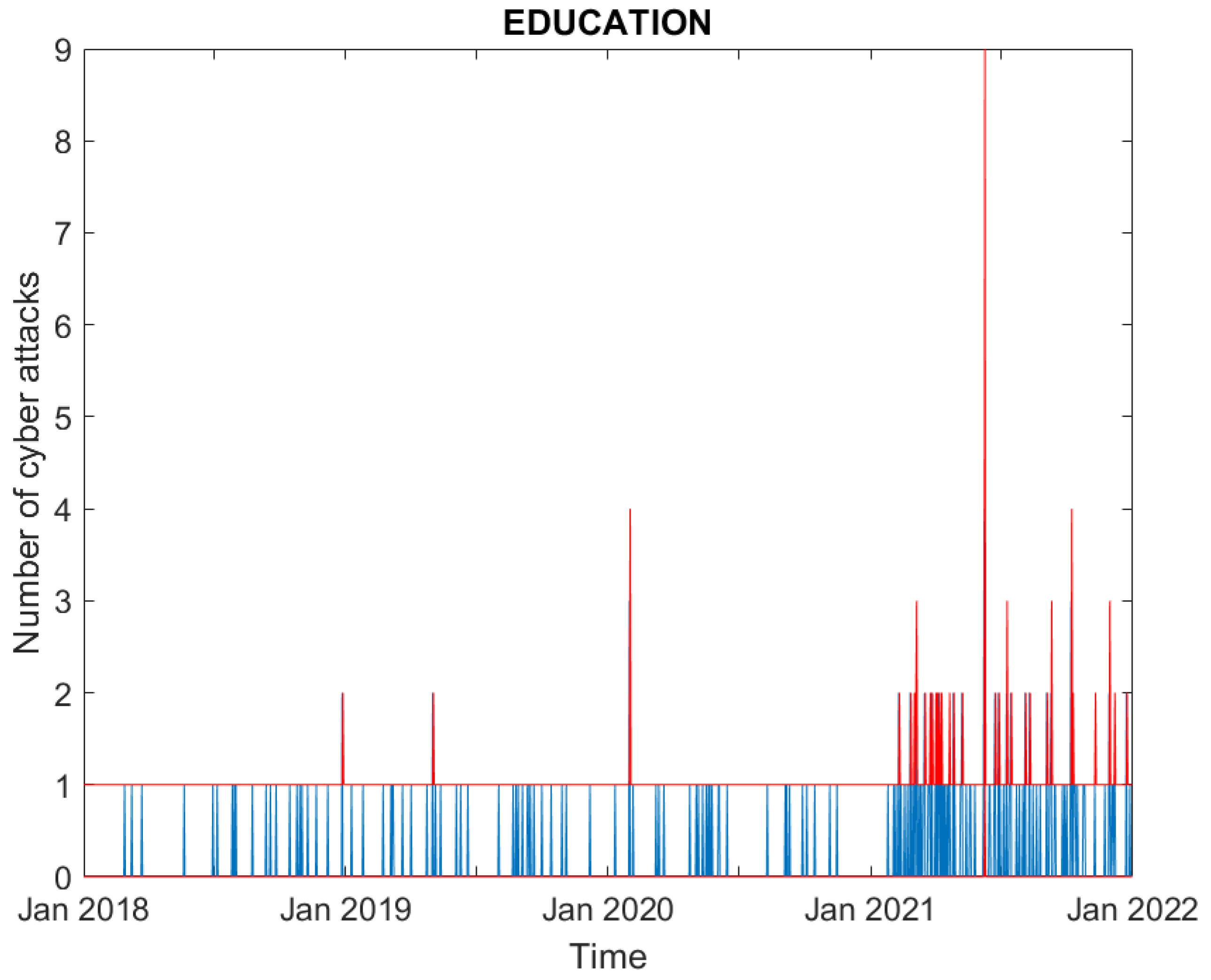
Figure 1. Real (blue) and predicted (95% confidence interval, red) cyber attack counts to education counterparties.
Risks 11 00165 g001
Figure 2. Real (blue) and predicted (95% confidence interval, red) cyber attack counts to government counterparties.
Risks 11 00165 g002
Figure 3. Real (blue) and predicted (95% confidence interval, red) cyber attack counts to healthcare counterparties.
Risks 11 00165 g003
Figure 4. Real (blue) and predicted (95% confidence interval, red) cyber attack counts to financial counterparties.
Risks 11 00165 g004
Figure 5. Real (blue) and predicted (95% confidence interval, red) cyber attack counts to ICT counterparties.
Risks 11 00165 g005
Figure 6. Real (blue) and predicted (95% confidence interval, red) cyber attack counts to trade counterparties.
Risks 11 00165 g006
Table 1. Maximum likelihood estimates of parameters for the multivariate negative binomial score-driven model applied to the daily count of “high” and “critical” severity cyber risk events in the 2018–2021 period (*** denotes statistical significance at the 1% level).
Sectorcb
Education−1.9443 ***0.1547 ***
(0.0639)(0.0202)
Government−0.3891 ***0.1086 ***
(0.0417)(0.0963)
Healthcare−0.3833 ***0.1086 ***
(0.0504)(0.0619)
Financial−0.3864 ***0.1085 ***
(0.0952)(0.0707)
ICT−0.3881 ***0.1086 ***
(−0.0612)(0.0906)
Trade−0.3868 ***0.1085 ***
(0.0345)(0.0504)
Table 2. Maximum likelihood estimate of the A matrix, expressing the in-sector and cross-sector impacts of shocks on the expected daily number of cyber risk events (EDU = education, GOV = government, HLT = healthcare, FIN = financial, ICT = information and communication technology, and TRD = trade). The bold numbers denote statistical significance at least at the 10% level.
SectorEDUGOVHLTFINICTTRD
EDU0.95480.00970.00150.00670.01050.0434
GOV0.00390.38340.00000.00340.00520.0217
HLT0.00610.00750.37980.00520.00810.0336
FIN0.01230.01520.00230.39100.01640.0680
ICT0.00000.00000.00120.00000.37880.0000
TRD0.00160.00200.00000.00140.00210.3890
Table 3. Percentage of violations of the upper 95% confidence interval and p-value of binomial test to compare it with the nominal percentage.
Sector% of Upper Confidence Interval ViolationsBinomial Test p-Value
EDU0.01710.0272
GOV0.03350.9817
HLT0.01440.0035
FIN0.00410.0000
ICT0.01570.0106
TRD0.00140.0000
Disclaimer/Publisher’s Note: The statements, opinions and data contained in all publications are solely those of the individual author(s) and contributor(s) and not of MDPI and/or the editor(s). MDPI and/or the editor(s) disclaim responsibility for any injury to people or property resulting from any ideas, methods, instructions or products referred to in the content.