The Generalised Pareto Distribution Model Approach to Comparing Extreme Risk in the Exchange Rate Risk of BitCoin/US Dollar and South African Rand/US Dollar Returns

Abstract

Cryptocurrencies are said to be very risky, and so are the currencies of emerging economies, including the South African rand. The steady rise in the movement of South Africans’ investments between the rand and BitCoin warrants an investigation as to which of the two currencies is riskier. In this paper, the Generalised Pareto Distribution (GPD) model is employed to estimate the Value at Risk (VaR) and the Expected Shortfall (ES) for the two exchange rates, BitCoin/US dollar (BitCoin) and the South African rand/US dollar (ZAR/USD). The estimated risk measures are used to compare the riskiness of the two exchange rates. The Maximum Likelihood Estimation (MLE) method is used to find the optimal parameters of the GPD model. The higher extreme value index estimate associated with the BTC/USD when compared with the ZAR/USD estimate, suggests that the BTC/USD is riskier than the ZAR/USD. The computed VaR estimates for losses of $0.07, $0.09, and $0.16 per dollar invested in the BTC/USD at 90%, 95%, and 99% compared to the ZAR/USD’s $0.02, $0.02, and $0.03 at the respective levels of significance, confirm that BitCoin is riskier than the rand. The ES (average losses) of $0.11, $0.13, and $0.21 per dollar invested in the BTC/USD at 90%, 95%, and 99% compared to the ZAR/USD’s $0.02, $0.02, and $0.03 at the respective levels of significance further confirm the higher risk associated with BitCoin. Model adequacy is confirmed using the Kupiec test procedure. These findings are helpful to risk managers when making adequate risk-based capital requirements more rational between the two currencies. The argument is for more capital requirements for BitCoin than for the South African rand.

1. Introduction

Investment in digital currencies, such as BitCoin, has been on a steady rise since the inception of cryptocurrencies globally and in South Africa. Cryptocurrencies are decentralised currencies that are traded on a blockchain technology platform without the regulations of a central bank. BitCoin tops the list of traded cryptoassets in terms of traded volume with a market capitalisation of 452.1 billion dollars (Tretina 2023).

Risk sentiment describes the risk appetite of market players (traders and investors), particularly their willingness (tolerance) to invest in a riskier asset or portfolio, e.g., risk sentiment towards emerging countries’ currencies (Grable 2000). Risk sentiment is important when the economic forecasts of one or some emerging countries are unfavourable, economic indicators are negative, and the markets are indicating a higher level of price instability. Some of the emerging economies maybe doing well economically but will still nonetheless have their currencies weakened or affected through such negative sentiment or through contagion (Fratzscher 2002). Investors move their currencies from emerging countries to “safe haven assets” which may not be affected by this negative sentiment around emerging countries (Almeida and Gonçalves 2023). South Africa is an emerging economy and is vulnerable to any negative sentiment around emerging economies (Davies 2017).

The South African rand is a central bank regulated currency; the South African Reserve Bank (SARB) moved towards a flexible exchange rate in 1994 (Van Der Merwe 1996). A flexible exchange rate allows market forces (supply and demand) to drive the pricing of currency, resulting in the rand experiencing a significant increase in volatility (Joale 2011). Thus, the rand is affected by speculation; hence, it is perceived as being risky (Pretorius and De Beer 2002).

Cryptocurrencies are said to be very risky (Kaseke et al. 2021). Emerging economies’ currencies, including the South African rand, are equally risky (Joale 2011). The question arises as to which of the two is riskier?

Extreme Value Theory is a field in statistics that measures and models extreme events (large fluctuations) using fat-tailed statistical distribution models. Risky assets have fat tails (more extreme observations than normal distribution allows for). Therefore, the application of EVT models is considered more appropriate to capture the financial risk of the BitCoin and rand exchange rates. This branch of statistics was pioneered by Fisher and Tippett (1928) and Pickands (1975). The purpose of this study is to fit the Extreme Value Theory (EVT)-based Generalised Pareto Distribution (the GPD) to estimate the Value at Risk (VaR) and the Expected Shortfall (ES). The two risk measures are used to compare the riskiness of the two assets. The GPD is preferred as it analyses extreme/tail-related risk.

Giving an analogy in a different field on the need to analyse extremes: “…why worry about the average rainfall, when it is extreme amounts of rainfall that cause a flood, or it is extreme low rainfall that causes a drought leading to untold suffering”. It makes sense to sometimes concentrate on analysing extremes as provided for in EVT. Classical statistical methodology often has an over-emphasis around the average or mean measure.

In measuring financial extreme risk using the EVT models, the Extreme Value Index (EVI) parameter dictates the tail behaviour of the returns’ distribution (Rached and Larsson 2019). This parameter signifies how the tail of the returns’ distribution decays (Beirlant et al. 2005).The parameter itself is a measure of risk when working with the EVT as loss distributions, and it also influences the estimation of the risk measures such as the Value at Risk (VaR) and Expected Shortfall (ES) (Penalva et al. 2016). A lot of studies have been conducted to refine the methods of estimating the EVI. Studies include those of Dekkers et al. (1989), Beirlant et al. (1996), Caeiro et al. (2005), Beirlant et al. (2005), and Cai et al. (2013).

The VaR is a statistical risk measure of a financial portfolio of assets. It is the largest value or amount expected to be lost over a specified time horizon, i.e., daily, weekly, or ten days, at a pre-defined statistical confidence level, p, and it quantifies the riskiness of an asset. Although investors and practitioners rely heavily on the VaR as a risk measure because of its ability to compress all Greeks to a single value (Hull 2006), it has shortcomings (Chou and Wang 2014). It is incoherent and also fails to precisely estimate the risk of loss when the loss distributions have ”fat tails”, unless EVT distributions are used (Rockafellar and Uryasev 2002). “This significantly discredits the accuracy of the traditional Normal distribution based VaR risk measure” (Chen 2018). To address the normal model distributional-related VaR weaknesses highlighted above, the EVT theory-based GPD is suggested in this study. Artzner et al. (1999) introduced a risk measure called the Expected Shortfall and called it “a perfect risk measure”. Pflug (2000) showed that the ES is a coherent risk measure.

However, it must be noted that the ES is not elicitable (Gneiting 2011), i.e., it does not minimise the expected loss function; thus, the measure may not be as accurate as estimates of the VaR (Yamai and Yoshiba 2002) and it is difficult to backtest (Hull 2006).

This paper uses the GPD model to compare the riskiness of BitCoin and South African rand returns using VaR and ES. Both currencies are measured against the US dollar. The steady rise in the movement of investments between the rand and BitCoin since the introduction of cryptocurrency influenced the selection of the two financial assets. The GPD model allows for the analysis of extreme gains and losses that may be associated with investing in BitCoin. The rand is also another developing country’s currency which is considered to be very risky. When analysing the extreme gains and losses, which of the two currencies is riskier?

The research will help foreign currency traders and investors to understand the extreme/tail risk they are taking when they convert their savings/investments to BitCoin instead of the South African currency, the rand. Furthermore, the findings are helpful to risk managers when making adequate risk-based capital requirements more rational between the two currencies. The argument is for more capital requirements for the riskier currency between the two exchange rates.

Literature Review

Several statistical risk/loss models have been developed to better capture the fat-tail property of financial assets in recent times. Yousof et al. (2023b) proposed a new reciprocal Weibull extension for modelling extreme values, Ibrahim et al. (2023) proposed a novel compound reciprocal Rayleigh extension model. Yousof et al. (2023a) proposed a novel flexible extension of the Chen distribution called the generalised Rayleigh Chen (GRC) and compared the performance of this new model with other Chen extension distributions, namely Gamma-Chen, Kumaraswamy Chen, Beta-Chen, Marshall–Olkin Chen, Transmuted Chen, and the traditional two-parameter Chen. Most of the distributions mentioned in this literature concentrate their fit around where most of the data are concentrated, around the average. Sometimes there is a need to depart from the average thinking and concentrate on the tails of statistical distributions. The GPD concentrates the distribution fit exclusively on these tails, allowing it to explore and explain extreme returns better than the various Weibull distributions mentioned herein.

In measuring financial tail-related risk using the EVT models, the Extreme Value Index (EVI) parameter dictates the tail behaviour of the returns’ distribution (Rached and Larsson 2019). This parameter is an indicator of how the tail of a distribution decays (Beirlant et al. 2005).The advantage of the GPD over the Weibull family models and related distributions, such as the exponential and Rayleigh models, lies in its ability to take a continuous range of possible shapes influenced by the EVI, which includes the exponential and Pareto distributions as special cases. The Generalised Pareto Distribution allows one to “let the data decide” which of these distributions is appropriate, instead of having to select a particular form of the parent distribution.

Balkema and de Haan (1974) and Pickands (1975) showed that for large enough thresholds, $u$’s, data exceedance distributions above these thresholds can be estimated by a Generalised Pareto Distribution (GPD). The Peak over Threshold (PoT) approach to the GPD involves selecting a threshold, $u$, and extracting values from the data that are considered extreme (exceedances above this threshold). The new data set is then used to create a model (the GPD) for the extreme values. To compute the VaR and ES, the GPD model parameters, including the EVI, must be estimated.

Studies are ongoing to determine the similarities of cryptocurrency features to those of other financial assets. Kaseke et al. (2021) detected some distributional similarities between cryptocurrencies, Gold and the FTSE/JSE 40, though the cryptocurrencies are slightly more volatile. Takaishi (2018) noted a fat-tail feature in BitCoin data. Bouri et al. (2017) observed a high volatility in BitCoin in comparison to other stock returns.

Dyhrberg (2016) argued that BitCoin and gold returns can be used for hedging as they are not affected by financial market shocks. Conversely, Shanaev and Ghimire (2021) noted a relative stability in BitCoin and Ethereum using asymmetric power-law statistical distributions.

This paper uses the GPD model to compare the riskiness of BitCoin and South African rand returns using VaR and ES. The GPD is preferred because of its ability to analyse extremes in returns and to take a continuous range of possible shapes influenced by the EVI.

2. Methodology

At times, there is a need to depart from the average and symmetrical thinking around losses and gains, and exploit information provided by the extreme returns. This helps to understand how extremes affect an investment. The survival of an investment company is not only influenced by the means of the distributions, but by the tails of distributions as well. Extreme losses can mean the investment company closes.

The Peak over Threshold (PoT) approach used in fitting the GPD is used to model extreme returns.

2.1. The Generalised Pareto Distribution (GPD)

Balkema and de Haan (1974) and Pickands (1975) showed that for large enough thresholds, $u$’s, the data exceedances above these thresholds can be estimated by the Generalised Pareto Distribution (GPD). The GPD is defined as follows:

$$G_{\xi ,\beta }\left(y\right)=\left\{\begin{array}{c}1-{\left(1+\frac{\xi (y-u)}{\beta }\right)}^{\raisebox{1ex}{$-1$}\!\left/ \!\raisebox{-1ex}{$\xi $}\right.} \mathrm{if} \xi \ne 0\\ 1-exp\left(-(\frac{y-u}{\beta })\right) \mathrm{if} \xi =0\end{array}\right.,$$

(1)

where $y$ are the returns series $y-u\ge 0$ for $\xi \ge 0$, $0\le y-u\le -\frac{\beta }{\xi }$, and $\xi <0$ after $0\le y-u\le -\beta /\xi$. $\xi$, is the extreme value index, and $\beta$ is the scale parameter. The value of $\xi$ measures the heaviness ofthe tail, with bigger positive values ($\xi$ > 0) indicating a heavy tail. When ($\xi$ < 0) is negative, the tail is short (bounded). $\xi$ = 0 indicates a light tail.

2.1.1. Parameter Estimation of GPD

For a reasonably high $u$ a subsample of n exceedances of observations, $y$, such that $y_i-u\ge 0$, the subsample $\{y_1-u,\dots .,y_n-u\}$ has an underlying distribution of a GPD. The logarithm of the probability density function of $y_i-u$ is:

$$\mathrm{l}\mathrm{n}\left(f\left(y_i-u\right)\right)=\left\{\begin{array}{l}-\ln \left(\beta \right)-\frac{1+\xi }{\xi }\ln \left(1+\xi \left(\frac{y_i-u}{\beta }\right)\right) \mathrm{if} \xi \ne 0\\ -\ln \left(\beta \right)-\frac{1}{\beta }\left(y_i-u\right) \mathrm{if} \xi =0\end{array}\right.$$

(2)

Then, the log-likelihood $L(\xi ,\beta |y_i-u)$ for the model is the logarithm of the joint density of the $n$ observations, i.e.,

$$L\left(\xi ,\beta |y_i-u\right)=\left\{\begin{array}{l}-n\ln \left(\beta \right)-\frac{1+\xi }{\xi }{\displaystyle \sum _{i=1}^n}\ln \left(1+\xi \left(\frac{y_i-u}{\beta }\right)\right) \mathrm{if} \xi \ne 0\\ -n\ln \left(\beta \right)-\frac{1}{\beta }{\displaystyle \sum _{i=1}^n}\left(y_i-u\right) \mathrm{if} \xi =0\end{array}\right.$$

(3)

We obtain the optimal values of the parameters $(\xi ,\beta )$ by maximising the log-likelihood function.

2.1.2. Excess Distribution

Let $Y$ be a random variable of returns with a density function, $F$, and the excess distribution above a certain threshold, $u$, is defined by (Balkema and de Haan 1974; Pickands 1975):

$$F_u\left(y\right)=\mathbb{P}\left(Y-u\le x|Y>u\right)=\frac{F\left(y+u\right)-F\left(u\right)}{1-F\left(u\right)}$$

(4)

where $(Y-u)$ is the size of exceedances over the threshold, u. $F_u\left(y\right)$ is the conditional excess distribution function. Smith (1987) showed that GPD-based formula for tail probabilities’ distribution is:

$${\widehat{F}}_u\left(y\right)=1-\frac{N_u}{n}{\left(1+\frac{\xi }{\beta }\left(y-u\right)\right)}^{\frac{-1}{\xi }}$$

(5)

where $n$ is the total sample size and $N_u$ is the number of exceedances above the threshold, $u$.

2.2. Risk Measures

For a small tail probability, p, and sample size, n, the formula for estimating VaR of returnsusing a GPD with optimal estimates $(\widehat{\beta },\widehat{\xi })$, threshold, $u$, and $N_u$ the number of exceedances, is given by:

$$\widehat{{VaR}_p}=\left\{\begin{array}{l}u+\frac{\widehat{\beta }}{\widehat{\xi }}\left\{1-{[-n\ln (1-p)]}^{-\widehat{\xi }}\right\} \mathrm{if} \widehat{\xi }\ne 0\\ u-\widehat{\sigma }\ln \left(-n\ln (1-p)\right) \mathrm{if} \widehat{\xi }=0\end{array}\right.$$

(6)

The Expected Shortfall is then given as:

$${ES}_p=\frac{{VaR}_p}{1-\widehat{\xi }}+\frac{\widehat{\beta }-\widehat{\xi }u}{1-\widehat{\xi }}$$

(7)

2.3. Model Adequacy

To validate the adequacy of the GPD, the estimation of VaR, the simple but effective (Zhang and Nadarajah 2017) unconditional coverage test by Kupiec (1995) is used.

The Kupiec test assumes that the proportion of failures of VaR estimates must be close to the corresponding tail probability level if the model is adequate. A failure is when the actual return is greater than VaR for upside risk, i.e., $y_t>{VaR}_p$, or less than VaR for downside risk, i.e., $y_t<{VaR}_p$.

Let $x^p$ be the number of violations, the test procedure involves comparing the corresponding proportion of violation [$\frac{x^p}{N}$] to p. The H₀: E$\left[\frac{x^p}{N}\right]=p$, i.e., (the expected proportion of violations is equal to $p$).

Under H₀, the Kupiec (1995) likelihood ratio test is:

$${LR}_{UC}=-2\mathit{ln}\left(\frac{p^{x^p}{\left(1-p\right)}^{N-x^p}}{{\left(\frac{x^p}{N}\right)}^{x^p}{\left(1-\frac{x^p}{N}\right)}^{N-x^p}}\right)~{\chi }^2(1),$$

(8)

where N is the total observations.

3. Results

Data on currency exchange rates utilised in this study came from the www.investing.com/currencies website (accessed on 1 July 2021), which serves the financial industry. R (R Core Team 2021), RStudio (RStudio Team 2022), rugarch (Ghalanos 2020), ismev (Heffernan and Stephenson 2018), and eva (Bader and Yan 2020) statistical programmes were used for the analysis. The GPD model was fitted with the daily adjusted closing prices from 1 January 2015 to 30 June 2021. The daily log returns were calculated and used for modelling. The formula used is $y_t=\log \left[\frac{P_t}{P_{t-1}}\right],$ where $P_t$ and $P_{t-1}$ are today and yesterday’s adjusted values, respectively.

In Figure 1 and Figure 2, the returns series are fairly stationary, around the zero-mean, while high and non-constant fluctuations are noticeable, indicating volatility clustering and heteroscedasticity. Isolated extreme returns are visible, suggesting the EVT models are relevant.

3.1. Descriptive Statistics

Table 1. Descriptive statistics of exchange rate price returns. Reproduced with permission from Chikobvu and Ndlovu (2023).

	Observations	Mean	Median	Maximum	Minimum	Skewness	Kurtosis
BTC/USD	2370	0.001990	0.001757	0.237220	−0.480904	−0.994382	16.15451
ZAR/USD	1694	−0.000125	0.000000	0.049546	−0.048252	−0.264130	4.121644
Test for normality, autocorrelation, and heteroscedasticity
		BTC/USD			ZAR/USD
TEST		Statistic	p-value		Statistic	p-value
Jarque–Bera		17,478.40	0.000000		108.4967	0.000000
Ljung–Box		11.7	0.0006249		0.40504	0.5245
ARCH LM Test		52.87	4.345 × 10−7		70.789	2.28 × 101
Test for unit root and stationarity
		BTC/USD			ZAR/USD
Unit Root Test		Statistic	p-value		Statistic	p-value
ADF Test		−52.20130	0.0001		−40.47263	0.0000
PP Test		−52.10963	0.0001		−40.47011	0.0000
KPSS Test		0.092067	0.347000		0.090747	0.347000

, below, gives a summary of the descriptive statistics.

In Table 1, the null hypothesis of normality using Jarque–Bera is rejected at the 5% level of significance. Thus, in this paper, a fat-tailed model, the GPD, is employed to capture non-normal features of the returns. The significant p-value of the Ljung–Box test for the ZAR/USD returns suggests the absence of autocorrelation. This means observations can be assumed to be independent and identically distributed (i.i.d). However, for the BTC/USD returns, this null hypothesis is rejected. The stationarity is confirmed using the Augmented Dickey–Fuller (ADF) and Phillips–Perron (PP) tests as the null hypothesis of a unit root is rejected at a 5% level of significance. The Kwiatkowski–Phillips–Schmidt–Shin (KPSS) test results show that all returns are stationary as well.

3.2. Data Analysis

The gains and losses are analysed separately. The losses are negative returns that were transformed using the formula $l_t=-1\times y_t.$ to make them positive. These losses are used in the analysis of the losses or lower tail of the return series.

The Pareto Q–Q plot and parameter stability plot approaches were used to select the threshold and extract extreme daily returns of the BitCoin and rand returns data using the PoT method. The gains (maxima) and losses (minima) were fitted to the GPD separately. The fitted models give estimates of the parameters ($\widehat{\xi }$, and $\widehat{\beta }$) and the estimated VaR and ES as measures of the tail-related risk for each scenario described.

3.2.1. Analysing the BTC/USD Returns

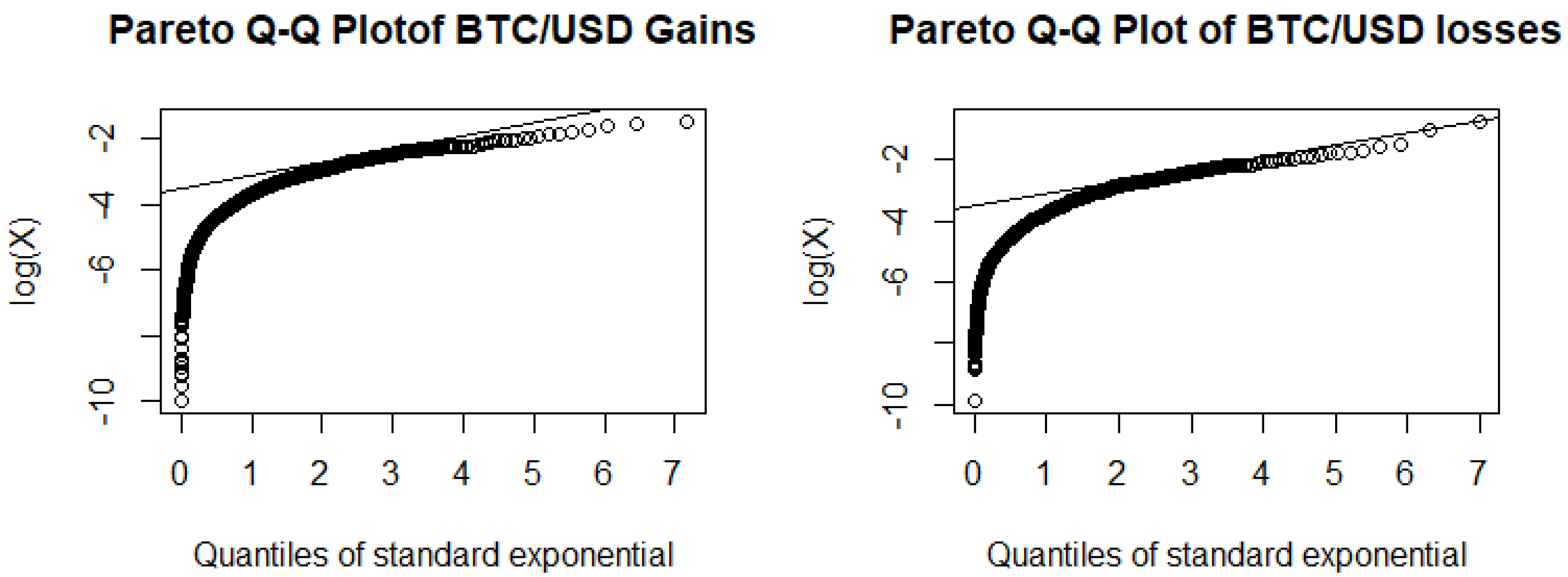
To fit the GPD model, a threshold, $u$, must be selected. The Pareto Q–Q plots determine a suitable threshold that is necessary for fitting the GPD model. The Pareto Q–Q plot method involves fitting a regression line to the data points in the Pareto Q–Q plot. The point where the fitted line cuts the vertical axis is the one that is used to estimate the threshold value in the data set. The exponent of the value where the regression line cuts through the vertical axis is taken as the threshold value. The straight line in Figure 3 shows the regression line for the BTC/USD gains (positive returns) and losses (negative returns).

Based on the observed threshold values of exp(−3.9) = 0.0202 and exp(−3.8) = 0.0224, we obtain 567 and 412 exceedances for the positive and negative log returns, respectively.

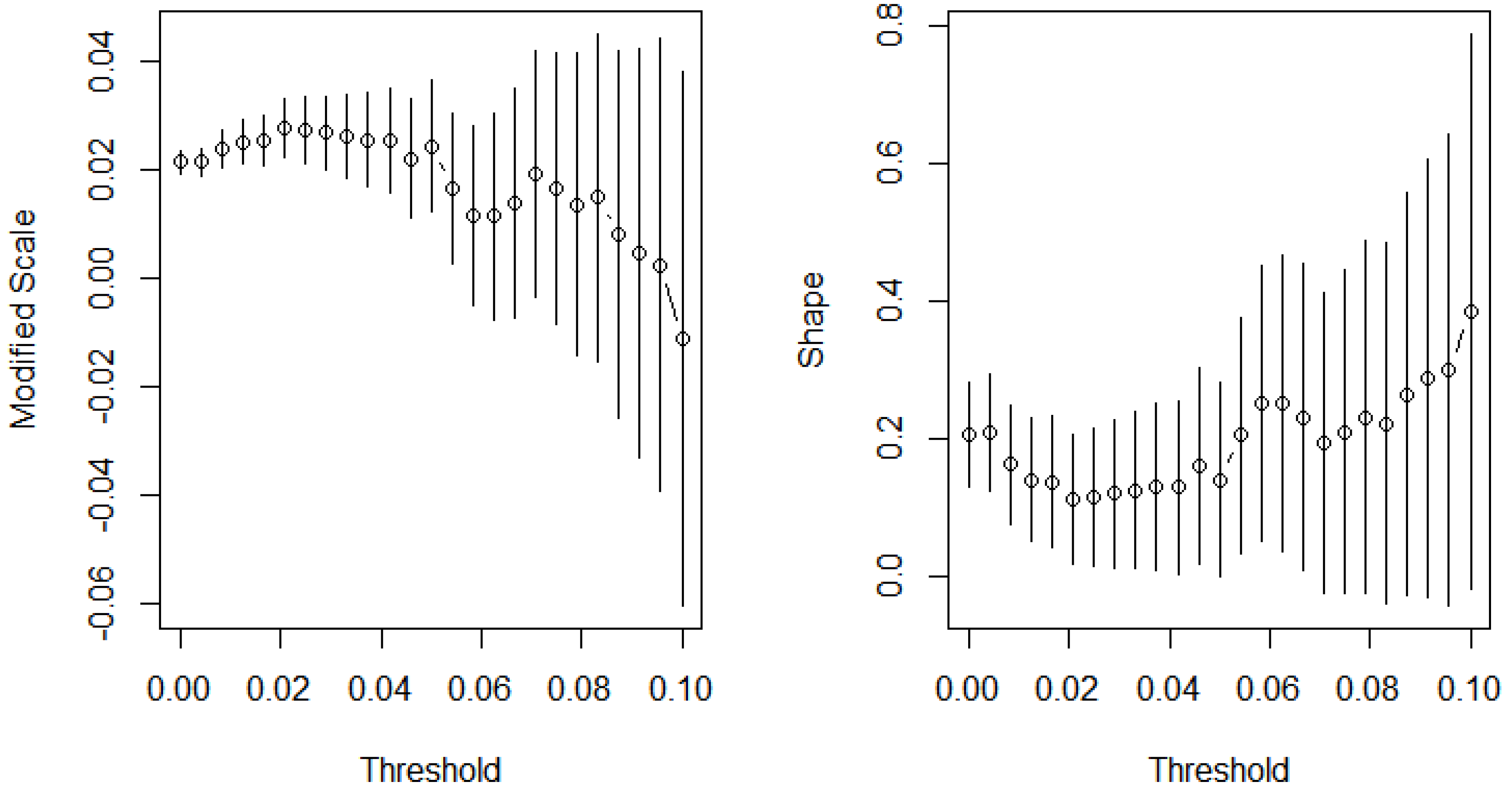
The stability in parameter approach is another method that helps ascertain a threshold that is neither too low (leading to bias in the model) nor too high (leading to high variance in parameters). Scarrott and MacDonald (2012) described stability in a parameter estimation method as stability in the threshold plot. This approach looks at the stability in the estimates of both the scale and shape parameter. The lowest value at which the plots of the estimates are approximately constant is taken to be the value at which the threshold value is found.

Based on the parameter stability plots of the shape and scale for the BTC/USD gains (positive returns) in Figure 4 and losses (negative returns) in Figure 5, the lowest value at which the plots of the estimates are approximately constant is approximately at 0.0202 and 0.0224. Hence, these values are confirmed to be reasonable.

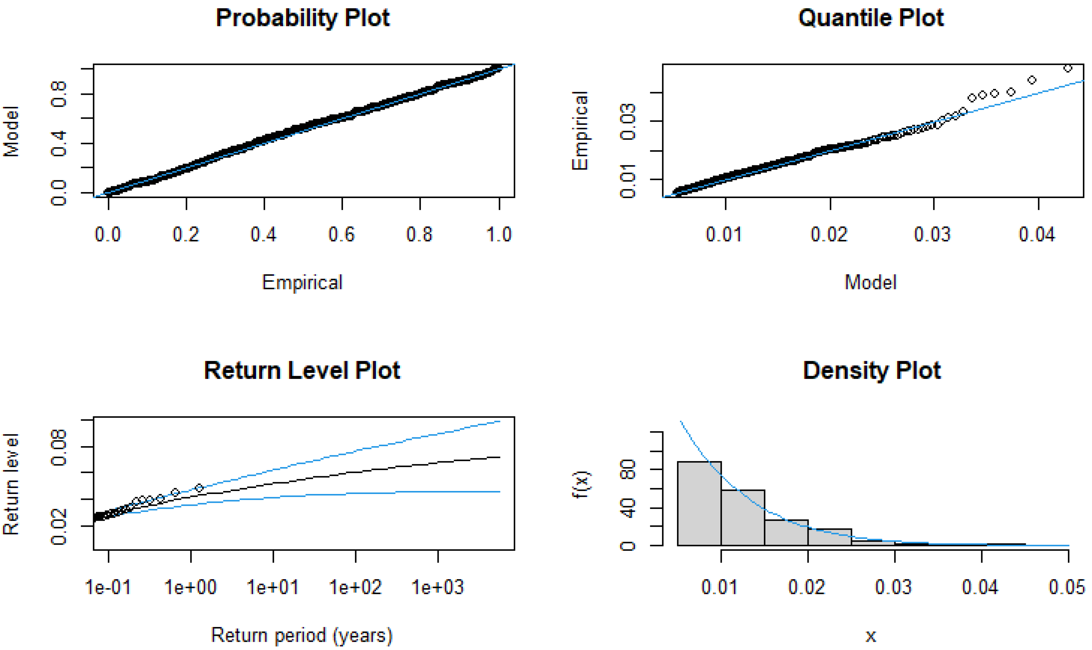
The diagnostic plots for the BTC/USD gains are presented in Figure 6. The quantile plots and probability plots do not deviate much from the straight line, suggesting that the GPD model is ideal for the upper tails of the BTC/USD. The return level plots indicate that there are no significant deviations from the curve, implying a good fit to the tail returns.

The diagnostic plots for the BTC/USD losses are presented in Figure 7. The quantile plots and probability plots do not deviate much from the straight line. The return level plots indicate that there are no significant deviations from the curve, implying that the GPD model is ideal for the lower tails of the BTC/USD.

3.2.2. Analysing ZAR/USD Returns

Figure 8 shows the Pareto Q–Q plots with fitted regression line for the ZAR/USD gains (positive returns) and losses (negative returns).

Based on Figure 8, the point where the fitted line cuts the vertical axis is the one that is used to estimate the threshold value in the data set. The exponents of the value where the regression line cuts through the vertical axis are exp(−5) = 0.0067 and exp(−5.3) = 0.0050, resulting in 391 and 520 exceedances for the positive and negative log returns, respectively.

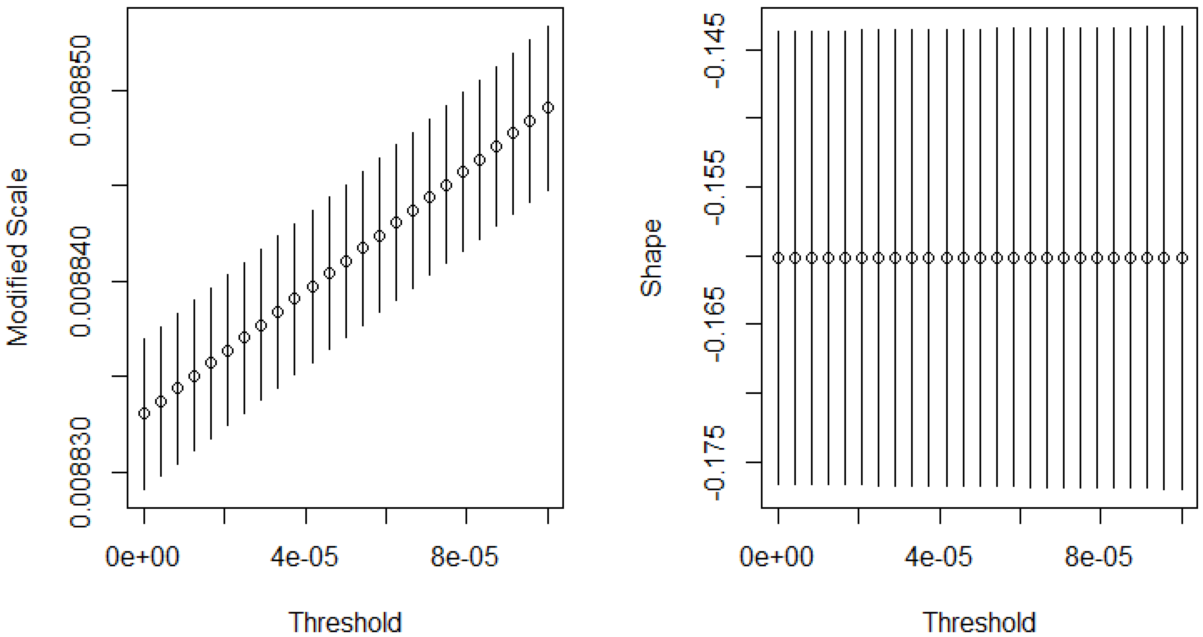
Based on the parameter stability plots of the shape and scale for the ZAR/USD gains (positive returns) in Figure 9, the lowest value at which the plots of the estimates are approximately constant is approximately at 0.0067. Hence, this value is confirmed to be reasonable. However, the stability plots of the shape and scale for the ZAR/USD losses (negative returns) in Figure 10 are inconclusive as the plots are showing stability at all points.

3.2.3. Model Diagnostics for the ZAR/USD Returns

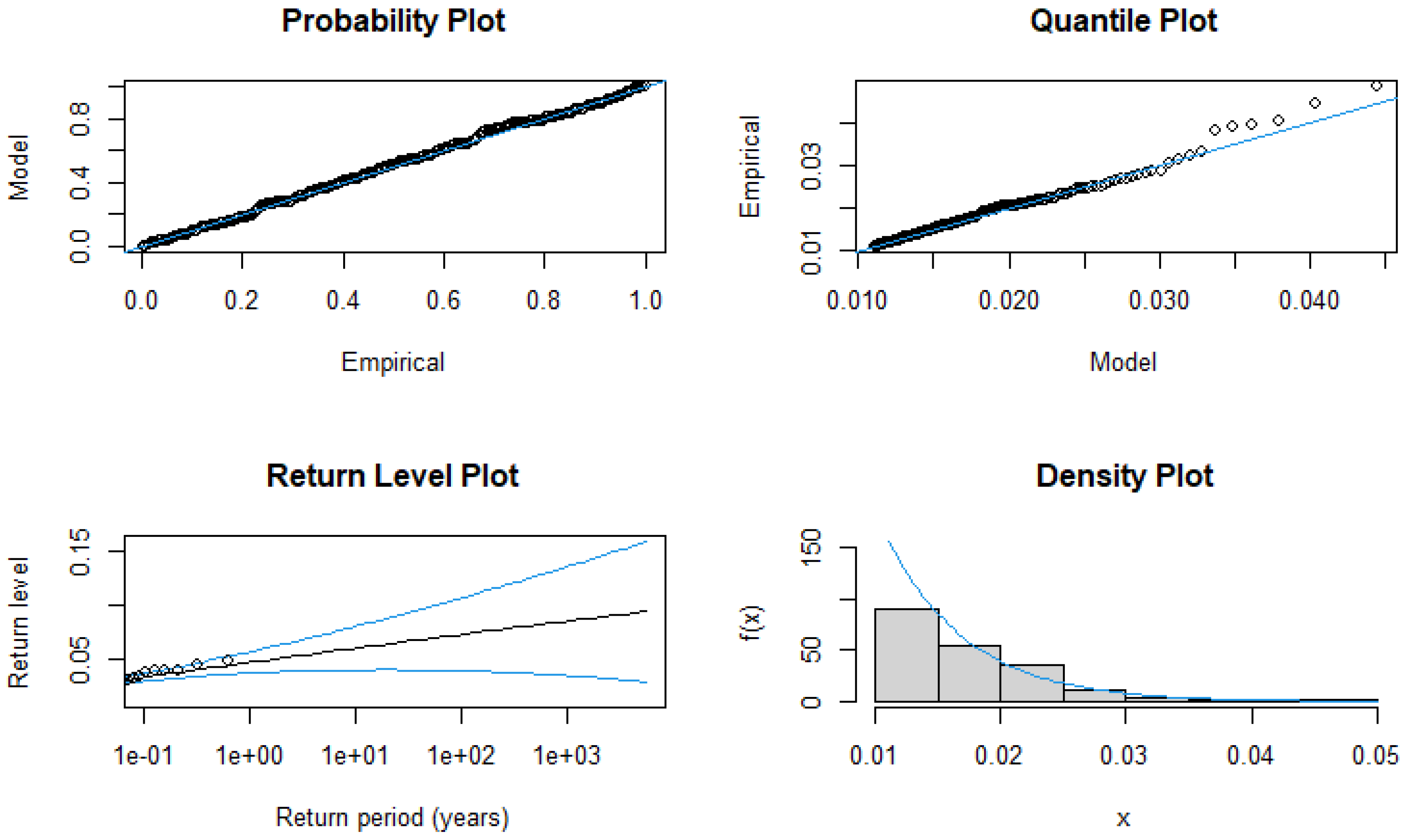
The diagnostic plots for the ZAR/USD gains are presented in Figure 11. The Q–Q and P–P plots do not deviate much from the straight line. The return level plots indicate that there are insignificant deviations from the curve, implying that the GPD model is ideal for the upper tails of the ZAR/USD.

The diagnostic plots for the ZAR/USD losses are presented in Figure 12. The Q–Q and P–P plots do not deviate much from the straight line. The return level plot shows that there are insignificant deviations from the curve, implying that the GPD model is ideal for the lower tails of the ZAR/USD.

3.3. Parameter Estimations

The Peaks over Thresholds of both currencies’ returns have been fitted to the GPD model.

Table 2. MLEs and SEs for GPD.

Model	Number of Exceedances	$\widehat{\mathit{\xi }}$	$\mathit{S}\mathit{e}\left(\widehat{\mathit{\xi }}\right)$	$\widehat{\mathit{\beta }}$	$\mathit{S}\mathit{e}\left(\widehat{\mathit{\beta }}\right)$
BTC/USD Gains	396	0.0302	0.0527	0.0284	0.0021
BTC/USD Losses	319	0.1096	0.0535	0.0311	0.0024
ZAR/USD Gains	229	−0.0164	0.0650	0.0005	0.0064
ZAR/USD Losses	243	−0.0844	0.0313	0.0065	0.0003

shows the MLEs of the parameters and their corresponding standard errors (SE).

All EVIs ($\widehat{\xi }’\mathrm{s}$) are positive (heavy-tailed) for both gains and losses in the case of the BTC/USD, implying that they follow a Pareto type heavy-tailed distribution. However, the EVIs ($\widehat{\xi }’\mathrm{s}$) are negative for both gains and losses in the case of the ZAR/USD, implying that they follow a Paretotype II-bounded distribution. The BTC/USD gains and losses have positive EVIs, i.e., on the gains, the BTC/USD $\widehat{\xi }$ is 0.0302 compared to the rand’s $\widehat{\xi }$ of −0.0164. The BTC/USD losses have $\widehat{\xi }=0.1096$ compared to the ZAR/USD’s $\widehat{\xi }=-0.0844$. BitCoin returns are heavy-tailed whilst the South African rand returns are bounded. This loosely indicates that BitCoin could be riskier than the rand, though further investigations (using VaR and ES) are required to quantify the relative risk in more appropriate terms, e.g., monetary terms.

3.4. Risk Measures

The VaR and ES estimates using the GPD model (see Equation (6) and (7)) are summarised in

Table 3. VaR Estimates.

	BTC/USD		ZAR/USD
	Losses	Gains	Losses	Gains
90%	0.07	0.06	0.02	0.02
95%	0.09	0.08	0.02	0.03
99%	0.16	0.13	0.03	0.03

and

Table 4. Expected Shortfall Estimates.

	BTC/USD		ZAR/USD
	Losses	Gains	Losses	Gains
90%	0.11	0.09	0.02	0.02
95%	0.13	0.11	0.02	0.03
99%	0.21	0.17	0.03	0.04

.

In Table 3, the BTC/USD tail-related losses of $0.07, $0.09, and $0.16 at 90%, 95%, and 99% confidence levels, respectively, are slightly greater than the expected tail-related gains of $0.06, $0.08, and $0.13, implying that there is a slightly higher downside risk associated with the BTC/USD than upside risk. However, for the ZAR/USD, the expected tail-related gains of $0.02, $0.03, and $0.03 are not different from the expected tail-related losses of $0.02, $0.02, and $0.03, except at a 95% confidence level, implying that the potential for gains and the potential for losses are offsetting each other for one invested in the ZAR/USD.

These estimates imply that the BTC/USD is riskier than the ZAR/USD for both gains and losses, because of the higher VaR and ES per US dollar invested in each currency. In Table 4, the ES (average losses) of $0.11, $0.13, and $0.21 per dollar invested in the BTC/USD at 90%, 95%, and 99% compared to the ZAR/USD’s $0.02, $0.02, and $0.03 at the respective levels of significance confirm the higher risk associated with BitCoin. The statement is true when the cryptocurrency (BitCoin) is compared to a developing country’s currency, the South African rand, which is perceived to be highly risky.

Although BitCoin is riskier than the rand, its mean the returns are greater than those of the ZAR/USD. This is consistent with mean-variance portfolio theory which suggests a higher yield for riskier assets (Markowitz 1959).

3.5. Model Adequacy

To confirm the adequacy of GPD-based VaR estimates, the Kupiec test (see Equation (8)) is employed. The p-values greater than 5% suggest that the model adequacy is achieved.

Table 5. Kupiec backtest results.

	BTC/USD		ZAR/USD
	Losses	Gains	Losses	Gains
90%	0.9901	0.96278	0.7140	0.9811
95%	0.6725	0.4288	0.420	0.5514
99%	0.3694	0.4212	0.8316	0.7375

summarises the findings.

Based on Table 5 above, the GPD fits fairly well to both the BTC/USD and ZAR/USD currency series’ gains and losses; hence, model adequacy is accepted at 95% and 99% since all p-values are greater than 5%. This overall acceptance of the GPD model underlines the robustness of EVT models in capturing the fat-tail features of the currencies and their high volatility, as described by Takaishi (2018).

4. Discussion

In this study, the GPD model is employed in the estimation of the Value at Risk (VaR) and Expected Shortfall (ES) in order to compare the riskiness of BitCoin and the South African rand, with both exchange rates measured against the US dollar. The BTC/USD returns exhibited heavy-tail behaviour in gains and losses, implying that the GPD is a good model offering a good fit for the tails of the distributions. The shape parameter, for instance, which is a useful tool for checking how heavy the tails are, gave values greater than zero, signifying the tails follow a heavy-tail Pareto type distribution (Penalva et al. 2016). However, for the ZAR/USD gains and losses, the EVI is negative, meaning the returns follow a bounded Pareto type II distribution. The EVT model provided a good fit to the tails of the distribution of the returns. The diagnostic plots showed that the probability and quantile plots do not deviate significantly from a straight line, signifying a good fit.

In Table 3 and Table 4, the VaR and ES estimates, respectively, lead one to conclude that BitCoin can give higher returns, but is also riskier than the rand.

The conclusion drawn from this study is that the BTC/USD exchange rate is riskier than the ZAR/USD exchange rate despite the rand being a developing country’s currency; hence, it is often perceived as being risky. The rand as hard cash is not convertible against major world currencies, but BitCoin is convertible. These findings are consistent with the fat-tail property associated with financial data by Danielsson (2011), and especially BitCoin (Takaishi 2018), and the high risk associated with cryptocurrencies (Kaseke et al. 2021). The high-risk, high-returns findings of Markowitz (1959) are also confirmed in these findings.

The findings are beneficial to local foreign currency traders and risk managers who need to fully appreciate the tail-related return and risk associated with converting their savings to BitCoin instead of keeping them in the local currency, the rand. Furthermore, these findings help risk managers make adequate risk-based capital requirements more rational between the two currencies. The argument is for more capital requirements for BitCoin than for the South African rand.

Limitations and Further Related Studies

It is important to emphasise that while this conclusion transcends time, but not assets, risk managers must model every asset (including other currencies of emerging markets) and compare their riskiness against their preferred cryptocurrency. Similarities to and, hence, conclusions regarding other developing countries can be inferred, but because each developing country has a unique currency riskiness, each study and conclusion must be conducted separately.

In an upcoming article, a hybrid of wavelets decomposition, GARCH, and EVT models will be investigated in order to enable more adaptable variance modelling by assessing the model’s sufficiency in gauging risks for the two financial assets.

References

1. Almeida, José, and Tiago Cruz Gonçalves. 2023. Portfolio Diversification, Hedge and Safe-Haven Properties in Cryptocurrency Investments and Financial Economics: A Systematic Literature Review. Journal of Risk and Financial Management 16: 3. [Google Scholar] [CrossRef]
2. Artzner, Philippe, Freddy Delbaen, Eber Jean-Marc, and David D. Heath. 1999. Coherent Measures of Risk. Mathematical Finance 9: 203–28. [Google Scholar] [CrossRef]
3. Bader, Brian, and Jun Yan. 2020. eva: Extreme Value Analysis with Goodness-of-Fit Testing. R Package Version 0.2.6. Available online: https://cran.r-project.org/web/packages/eva/eva.pdf (accessed on 10 December 2022).
4. Balkema, August A., and Laurens de Haan. 1974. Residual lifetime at great age. Annals of Probability 2: 792–804. [Google Scholar] [CrossRef]
5. Beirlant, Jan, Petra Vynckier, and Jozef L. Teugels. 1996. Tail index estimation, Pareto quantile plots, and regression diagnostics. Journal of American Statistical Association 91: 1659–67. [Google Scholar]
6. Beirlant, Jan, Goedele Dierckx, and Armelle Guillou. 2005. Estimation of the extreme-value index and generalized quantile plots. Bernoulli 11: 949–70. [Google Scholar] [CrossRef]
7. Bouri, Elie, Peter Molnár, Georges Azzi, David Roubaud, and Lars Ivar Hagfors. 2017. On the hedge and safe haven properties of BitCoin: Is it really more than a diversifier? Finance Research Letters 20: 192–98. [Google Scholar] [CrossRef]
8. Caeiro, Frederico, Maria Ivette Gomes, and Dinis Pestana. 2005. Direct reduction of bias of the classical hill estimator. Revstat 3: 113–36. [Google Scholar]
9. Cai, Juan-Juan, Laurens de Haan, and Chen Zhou. 2013. Bias correction in extreme value statistics with index around zero. Extremes 16: 173–201. [Google Scholar] [CrossRef]
10. Chen, James Ming. 2018. On Exactitude in Financial Regulation: Value-at-Risk, Expected Shortfall, and Expectiles. Risks 6: 61. [Google Scholar] [CrossRef]
11. Chikobvu, Delson, and Thabani Ndlovu. 2023. The Generalised Extreme Value Distribution Approach to Comparing the Riskiness of BitCoin/US Dollar and South African Rand/US Dollar Returns. Journal of Risk and Financial Management 16: 253. [Google Scholar] [CrossRef]
12. Chou, Heng-Chih, and David K. Wang. 2014. Estimation of Tail-Related Value-at-Risk Measures: Range Based Extreme Value Approach. Quantitative Finance 14: 293–304. [Google Scholar] [CrossRef]
13. Danielsson, Jon. 2011. Financial Risk Forecasting. London: Wiley. [Google Scholar]
14. Davies, Martyn. 2017. Is South Africa the Next Brazil? Emerging Market Insights. Available online: https://www2.deloitte.com/content/dam/Deloitte/za/Documents/africa/DeloitteZA_Is_South_Africa_the_next_Brazil_Sep2017.pdf (accessed on 2 May 2023).
15. Dekkers, Arnold L. M., John H. J. Einmahl, and Laurens de Haan. 1989. A moment estimator for the index of an extreme-value distribution. Annals of Statistics 17: 1833–55. [Google Scholar] [CrossRef]
16. Dyhrberg, Anne Haubo. 2016. BitCoin, gold and the dollar—A Garch volatility analysis. Finance Research Letters 16: 85–92. [Google Scholar] [CrossRef]
17. Fisher, Ronals, and Leonard Tippett. 1928. Limiting forms of the frequency distribution of the largest or smallest member of a sample. Mathematical Proceedings of the Cambridge Philosophical Society 24: 180–90. [Google Scholar] [CrossRef]
18. Fratzscher, Marcel. 2002. On Currency Crises and Contagion. Working Paper Series 139; Franfurt am Main: European Central Bank. [Google Scholar]
19. Ghalanos, Alexios. 2020. rugarch: Univariate GARCH Models. R Package Version 1.4-4. Available online: https://cran.r-project.org/web/packages/rugarch/index.html (accessed on 10 December 2022).
20. Gneiting, Tilmann. 2011. Making and evaluating point forecasts. Journal of the American Statistical Association 106: 746–62. [Google Scholar] [CrossRef]
21. Grable, John. 2000. Financial risk tolerance and additional factors that affect risk taking in everyday money matters. Journal of Business and Psychology 14: 625–30. [Google Scholar] [CrossRef]
22. Heffernan, Janet E., and Alec G. Stephenson. 2018. ismev: An Introduction to Statistical Modeling of Extreme Values. R Package Version 1.42. Available online: https://cran.r-project.org/web/packages/ismev/ismev.pdf (accessed on 10 December 2022).
23. Hull, John. 2006. Risk Management and Financial Institutions, 1st ed. Hoboken: Prentice Hall. [Google Scholar]
24. Ibrahim, Mohamed, Walid Emam, Yusra Tashkandy, Mir Masoom Ali, and Haitham M. Yousof. 2023. Bayesian and Non-Bayesian Risk Analysis and Assessment under Left-Skewed Insurance Data and a Novel Compound Reciprocal Rayleigh Extension. Mathematics 11: 1593. [Google Scholar] [CrossRef]
25. Joale, Dan. 2011. Analyzing the Effect of Exchange Rate Volatility on South Africa’s Exports to the US—Theory and Evidence. SSRN Electronic Journal. [Google Scholar] [CrossRef]
26. Kaseke, Forbes, Shaun Ramroop, and Henry Mwambi. 2021. A Comparison of the Stylised Facts of BitCoin, Ethereum and the JSE Stock Returns. African Finance Journal 23: 50–64. [Google Scholar]
27. Kupiec, Paul H. 1995. Techniques for verifying the accuracy of risk management models. Journal of Derivatives 3: 73–84. [Google Scholar] [CrossRef]
28. Markowitz, Harry. 1959. Portfolio Selection: Efficient Diversification of Investments. New York: John Wiley & Sons. [Google Scholar]
29. Penalva, Helena, Sandra Nunes, and Manuela M. Neves. 2016. Extreme Value Analysis—A Brief Overview With an Application to Flow Discharge Rate Data in A Hydrometric Station In The North Of Portugal. REVSTAT—Statistical Journal Volume 14: 193–215. [Google Scholar]
30. Pflug, Georg Ch. 2000. Some Remarks on the Value-at-Risk and the Conditional Value-at-Risk. Probabilistic Constrained Optimization. Boston: Springer, pp. 272–81. [Google Scholar]
31. Pickands, James, III. 1975. Statistical inference using extreme order statistics. Annals of Statistics 3: 119–31. [Google Scholar] [CrossRef]
32. Pretorius, Anmar, and Jesse De Beer. 2002. Financial Contagion in Africa: South Africa and a Troubled Neighbour, Zimbabwe. Paper presented at the 7th Annual Conference of the African Econometrics Society, Kruger National Park, South Africa, June 19–23. [Google Scholar]
33. R Core Team. 2021. R: A Language and Environment for Statistical Computing. Vienna: R Foundation for Statistical Computing. Available online: https://www.R-project.org/ (accessed on 1 December 2021).
34. Rached, Imen, and Elisabeth Larsson. 2019. Tail Distribution and Extreme Quantile Estimation Using Non-parametric Approaches. In High-Performance Modelling and Simulation for Big Data Applications. Cham: Springer, vol. 11400. [Google Scholar] [CrossRef]
35. Rockafellar, Ralph Tyrrell, and Stan Uryasev. 2002. Conditional value-at-risk for general loss distributions. Journal of Banking & Finance 26: 1443–71. [Google Scholar] [CrossRef]
36. RStudio Team. 2022. RStudio: Integrated Development Environment for R. Boston: RStudio, PBC. Available online: http://www.rstudio.com/ (accessed on 10 December 2022).
37. Scarrott, Carl, and Anna MacDonald. 2012. A Review of Extreme Value Threshold Estimation and Uncertainty Quantification. REVSTAT-Statistical Journal 10: 33–60. [Google Scholar]
38. Shanaev, Savva, and Binam Ghimire. 2021. A fitting return to fitting returns: Cryptocurrency distributions revisited. SSRN Electronic Journal 1: 1–33. [Google Scholar] [CrossRef]
39. Smith, Richard L. 1987. Estimating Tails of Probability Distributions. The Annals of Statistics 15: 1174–207. [Google Scholar] [CrossRef]
40. Takaishi, Tetsuya. 2018. Statistical properties and multifractality of BitCoin. Physica A: Statistical Mechanics and Its Applications 506: 507–19. [Google Scholar] [CrossRef]
41. Tretina, Kat. 2023. Top 10 Cryptocurrencies of 2023. Forbes Advisor. Available online: https://www.forbes.com/advisor/investing/cryptocurrency/top-10-cryptocurrencies/ (accessed on 7 March 2023).
42. Van Der Merwe, E. 1996. Exchange Rate Management Policies in South Africa: Recent Experience and Prospects. South African Reserve Bank Occasional Paper No. 8, June 1995. Pretoria: South African Reserve Bank Occasional. [Google Scholar]
43. Yamai, Yasuhiro, and Toshinao Yoshiba. 2002. Comparative Analysis of Expected Shortfall and Value at Risk: Their Estimation Error, Decomposition, and Optimization. Monetary and Economic Studies 20: 87–121. [Google Scholar]
44. Yousof, Haitham M., Walid Emam, Yusra Tashkandy, Mir Masoom Ali, Richard Minkah, and Mohamed Ibrahim. 2023a. A Novel Model for Quantitative Risk Assessment under Claim-Size Data with Bimodal and Symmetric Data Modeling. Mathematics 11: 1284. [Google Scholar] [CrossRef]
45. Yousof, Haitham M., Yusra Tashkandy, Walid Emam, Mir Masoom Ali, and Mohamed Ibrahim. 2023b. A New Reciprocal Weibull Extension for Modeling Extreme Values with Risk Analysis under Insurance Data. Mathematics 11: 966. [Google Scholar] [CrossRef]
46. Zhang, Yuanyuan, and Saralees Nadarajah. 2017. A review of backtesting for value at risk. Communications in Statistics—Theory and Methods 47: 3616–39. [Google Scholar] [CrossRef]
Figure 1. Plot of BTC/USD prices (left) and one-day log returns (right). Reproduced with permission from Chikobvu and Ndlovu (2023).
Risks 11 00100 g001
Figure 2. Plot of ZAR/USD prices (left) and one-day log returns (right). Reproduced with permission from Chikobvu and Ndlovu (2023).
Risks 11 00100 g002
Figure 3. The Pareto Q–Q plots for the BTC/USD returns’ gains and losses.
Risks 11 00100 g003
Figure 4. Parameter stability plots of the shape and scale parameter forBTC/USD gains.
Risks 11 00100 g004
Figure 5. Parameter stability plots of the shape and scale parameter forBTC/USD losses.
Risks 11 00100 g005
Figure 6. The model diagnostics plots of the BTC/USD gains.
Risks 11 00100 g006
Figure 7. The model diagnostics plots of the BTC/USD losses.
Risks 11 00100 g007
Figure 8. The Pareto Q–Q plots for the ZAR/USD gains and losses.
Risks 11 00100 g008
Figure 9. Parameter stability plots of the shape and scale parameter forZAR/USD gains.
Risks 11 00100 g009
Figure 10. Parameter stability plots of the shape and scale parameter for ZAR/USD losses.
Risks 11 00100 g010
Figure 11. The model diagnostics plots of the ZAR/USD gains.
Risks 11 00100 g011
Figure 12. The model diagnostics plots of the ZAR/USD losses.
Risks 11 00100 g012