Dependency Modeling Approach of Cause-Related Mortality and Longevity Risks: HIV/AIDS

Abstract

Disaggregation of mortality by cause has advanced the development of life tables for life insurance and pension purposes. However, the assumption that the causes of death are independent is a challenge in reality. Furthermore, models that determine relationships among causes of death such as HIV/AIDS and their impact on mortality and longevity risks seem trivial or inflexible. To address these problems, we aim to determine and build an appropriate copula dependence model for HIV/AIDS against other causes of death in the presence of age, gender, and time. A bivariate copula model is proposed to capture the dependence structure of HIV/AIDS on life expectancy. This approach allows the fitting of flexible and interpretable bivariate copulas for a two-dimensional case. The dataset was derived from the World Health Organization database that constituted annualized death numbers, causes, age, gender, and years (2000 to 2019). Using Kendall’s tau and Pearson linear coefficient values, the survival Joe copulas proved to be a suitable model. The contribution and implication of this research are the quantification of the impact of HIV/AIDS on a life table, and, thus, the establishment of an alternative to the subjective actuarial judgment approach.

1. Introduction

Causes of death data in insurance have grown to be considered a critical input in estimating mortality and longevity risks in actuarial studies as used in epidemiology and biostatistics (Stracke and Heinen 2020). In particular, the pricing of life insurance and pension contracts requires mortality and longevity projections in developing life tables and thus, cause-based life tables have recently become invaluable (Murphy et al. 2021). Life tables can be classified based on model formulation, that is, using the aggregate death or the disaggregate causes of death mortality. The functional approach between the two is based on the risk studied and the underlying life insurance benefit. However, causes of death mortality models are constrained by the assumption of independence (Kjærgaard et al. 2019). Studies have demonstrated that there exists inherent dependency among causes, and thus reality may not hold (Kaishev et al. 2007; Chiang 1968).

Life insurance pays in the case of natural or accidental deaths. Natural deaths encompass the majority of causes; however, in some instances, deaths linked to suicide are excluded. In the United States, the Accidental Death and Dismemberment Policy (AD&D) and the Accidental Death Benefits (ADB) (Richmond 2009; Mueller 2004) pay claims due to accidental causes of deaths and injuries as defined in the policy. Such policies also act as riders to the main life insurance product to increase the final benefit payout. Additionally, a critical illness insurance policy takes effect on the occurrence of a defined list of diseases. These benefits would require different pricing life tables, such as the multiple decrement life tables. According to Beltrán-Sánchez et al. (2008), these mortality tables are referred to as the cause-deleted life tables or Associated Single Decrement Life Tables (ASDLT).

The impact of certain causes of death on a mortality life table has lacked a quantified approach, and thus actuarial judgments have relied on subjective principles. The conservatism approach employed by actuaries has continued to be the main technique in determining the extent of the impact of unquantified risks (Strauss et al. 2005). The aims of this approach are to alleviate basis risk in pricing, reserving, and valuation of life products. If the actuary is optimistic then the premiums or contributions will become less in the earlier years but will be increased in the latter years, alternatively, if the actuary is pessimistic then the premiums or contributions of the benefit will be higher than normal at the onset and reduce in the future. Life tables are affected by subjectiveness, for instance, mortality and longevity provisions are adjusted based on judgment of the prevailing mortality assumptions. In developing life tables in Kenya, a conservatism approach is considered in accounting for HIV/AIDS’ impact on the life table. To minimize this risk of subjective judgment by actuaries, a dependence model would thus be suggested to enable and enhance improvement in understanding the impact of deaths due to HIV/AIDS on a lifetable.

HIV/AIDS has shown a tremendous decline in being a leading cause of death for the past 20 years not only in entire Sub-Saharan Africa but more specifically in Kenya. Bett et al. (2022) have shown that for both males and females across all ages, HIV/AIDS has consistently portrayed a decreasing trend in the future. Measurement of the exact gain or loss to a life table is still to the best of our knowledge unquantified. The earliest Kenyan life tables were the A1949-52 mortality tables derived from the United Kingdom (UK) and Wales due to a similar mortality experience in Kenya as in the UK then. The KE 2001–2003 Tables for Assured Lives were published in 2011 and have been widely used, but have failed to capture the immense improvement in life expectancy despite the adjustment to HIV/AIDS. Model life tables include UN (1958, 1982), Coale and Demeny (1966, 1983), INDEPTH AIDS, decremented model life tables, and Weiss 1973 (Obscure anthropological model life tables), which have also been employed by the United Nations to estimate the extent of mortality on life tables and all rely heavily on assumptions. The interactions of causes of death with the aggregate deaths would be a key study to establish the correlation structure of specific causes of death with other causes, and this can be achieved by using copulas. Cause-eliminated life tables are created in the framework of the competing risks model where the relationships among competing events are assessed and measured in relation to other events of interest. Therefore, studying the dependence structure of HIV/AIDS using copulas would aid in understanding the future evolution of mortality and longevity risk and, consequently, the dependence structure. Additionally, Kaishev et al. (2007) noted in their paper that extensions of the copulas approach to newer causes such as HIV/AIDS would be relevant.

There are two main types of mortality and longevity models in actuarial literature, that is, extrapolative and explanatory approaches. The former method has been shown to be cautionable as demonstrated by Bengtsson and Keilman (2019) on the trends in life expectancy among women in Denmark and the Netherlands. Life expectancy from 1970 was overestimated as compared to other European countries because the extrapolation model failed to foresee trends, cause approach is thus preferred. Cause of death mortality models, for instance, vector error correction models (VECM), were developed to track the long-term association of the causes of death based on co-integrating relationships (Alai et al. 2013; Arnold and Sherris 2015). Co-integration (Engle and Granger 1987) is the long-term linear combination of integrated time series based on deterministic or stochastic trends. Modeling the multivariate dependence modeling structure takes the short-term correlation into account and ensures that the time dependence of the correlation is identified. For co-integration, the relationship must be longer to ensure validity in the co-integration relationship; however, the lack of sufficient long-term data hampers the robustness of the model.

The differentiation of correlation and co-integration is based on the time frame of the data, and thus co-integration is more suitable for long-term relationships while correlation is suitable for short-term ones. Copulas and co-integration techniques have been compared in financial stocks by Stander et al. (2013). It was found that the copula approach was more suitable for the short-term asset allocation approach as compared to the long-term co-integration approach.

Therefore, the purpose of this study is to determine the copula structure that exists between key causes of death that influence mortality and longevity risks and apply it to a cause-eliminated life table, particularly HIV/AIDS. This is because instead of only checking correlation, a copula structure would enable the illustration of profound relationships among covariates that can be measured.

This paper has been divided into four parts. The next section deals with copulas as applicable in mortality modeling, Section 3 will be methods and materials, followed by results and discussions in Section 4, and finally, the conclusion and future work in Section 5.

2. Copulas in Mortality Modelling

There exist three types of copulas: fundamental, implicit, and explicit (McNeil et al. 2015). The fundamental case involves the independence copula, the implicit case is the Gaussian and the Student-t copula, and the explicit type is the Archimedean copula family that includes the Frank, Gumbel, and Clayton copulas (Kaishev et al. 2007; Li and Lu 2018; Nelsen 2007) and others; all of these are applied based on the structure of the data. Exploration of bivariate distributions between the aggregate death rate and the individual causes would therefore enable us to obtain key relationships of interest.

Mortality data, specifically, shows that the causes of death have complex dependent structures that are non-symmetric, meaning that they are not linear in structure. Therefore, they may fail to be captured by the independence or the implicit multivariate normal copulas (Gaussian), and thus a flexible dependent model would suffice to understand the inherent complexities among the causes of death. Additionally, the challenge with the implicit Gaussian approach is that it fails to account for asymmetrical, extreme, and heavy-tailed distributions.

On the other hand, the explicit Archimedean copulas are rigid in nature and fail to allow differing dependency structures among variables. The hierarchical Archimedean copula model (Li and Lu 2018) was applied in life insurance; however, the complexities of the model have continued to render the model less applicable in practice. Due to the different complex marginals among individual variables and the non-symmetric dependencies of the individual pairs, a flexible copula structure is thus needed; consequently, the multivariate copulas that include rotated, survival, and tawn copulas have been developed to enhance flexibility with minimized complexities (Bedford and Cooke 2002; Aas et al. 2009). They are constructed from bivariate (pair) copulas and scaled to incorporate more variables of interest. They are feasible and applicable in reality because they allow the use of the conditioning approach.

2.1. Copula Definition

According to McNeil et al. (2015), $d$-dimensional copula is a distribution function on ${\left[0,1\right]}^d$ with a standard uniform marginal distribution. Let $C\left(u\right)=C(u_1,\dots ,u_d)$ be the multivariate distribution functions that are copulas. Mapped as $C:{[0,1]}^d\to [0,1]$ with the following three conditions:

(1)

$C(u_1,\dots ,u_d)$ is increasing in each $u_i$

(2)

$C\left({1,\dots ,1,u}_i,\dots 1\right)=u_i$ such that $\forall i\in \left\{1,\dots ,d\right\},u_i\in [0,1]$

(3)

$\forall$ $(a_1,\dots ,a_d)$, $(b_1,\dots ,b_d)$ $\in {\left[0,1\right]}^d$ with $a_i\le b_i$ we have the following:

$${\sum }_{i_1=1}^2\cdots {\sum }_{i_d=1}^2{\left(-1\right)}^{i_1+\dots +i_d}C\left(u_{1i_1},\dots ,u_{d{i}_d}\right)\ge 0,$$

(1)

where $u_{j1}=$ $a_j$ and $u_{j2}=$ $b_j$ $\forall$ $j\in \left\{1,\dots ,d\right\}.$

The third condition is the rectangle inequality that ensures a non-negative probability, that is, $P\left(a_1\le U_1\le b_1,\dots ,a_d\le U_d\le b_d\right)\ge 0$.

2.2. Sklar Theorem

A key result involving copulas is Sklar’s theorem (Sklar 1973), which states that any multivariate joint distribution can be written in terms of univariate marginal distribution functions and a copula, which describes the dependence structure between the two variables. The Sklar theorem enables a connection to exist between the multivariate distribution functions and the univariate margins. The theorem of Copulas is achieved and holds based on Sklar (1959) and it states that a multivariate distribution function F can be written in the form of a copula function such that if $F(x_1,x_2,\dots ,x_d)$ is a joint multivariate distribution function with univariate marginal distributions functions $F_1{x}_1$, $F_2{x}_2$, …, $F_d{x}_d$ then there exists a copula function $C(u_1,\dots ,u_d)$ such that:

$F(x_1,x_2,\dots ,x_d)$ = $C(F_1{x}_1$, $F_2{x}_2$, …, $F_d{x}_d$) if each $F_i$ is continuous then $C$ is unique.

Frechet bounds (Fréchet 1951) explains limits of both the maximum and minimum bounds in a copula function are given by:

$$max\left(0,u+v-1\right)\le C(u,v)\le min(u,v).$$

(2)

Let $T_1,\dots ,T_n$, 0 $\le T_j<\omega$, $j=1,\dots ,n$ represent the future lifetime random variable with a maximum time limit, $\omega$, due to cause of death j for n total causes. Further, let $\min (T_1,\dots ,T_n)$ represent the actual random lifetime. Thus, the joint distributions that represent the lifetime distribution function will be:

$$F\left(t_1,\dots ,t_n\right)=\mathrm{P}\mathrm{r}\{T_1\le t_1,\dots ,T_n\le t_n\}$$

and the joint survival function:

$$S\left(t_1,\dots ,t_n\right)=\mathrm{P}\mathrm{r}\{T_1>t_1,\dots ,T_n>t_n\}.$$

These random variables will be considered dependent and non-defective such that

$$\mathrm{Pr}\left\{T_j<\omega \right\}=1.$$

2.3. Complete Cause Elimination

The impact of a complete cause elimination and its quantification will be of interest, similar to the procedure of Elandt-Johnson (1976), who demonstrated cause elimination by considering the marginal distribution of the individual cause of death. Assuming that we remove cause i the resultant survival function becomes:

$F\left(t_1,\dots ,t_{i-1},t_{i+1},\dots ,t_n\right)=\mathrm{P}\mathrm{r}\{T_1\le t_1,\dots ,{T_{i-1}\le t}_{i-1},T_{i+1}\le t_{i+1},\dots ,T_n\le t_n\}$ where $i$ is removed and letting,

$$S^{\left(-i\right)}\left(t\right)=S\left(t_1,\dots ,t_{i-1},t_{i+1},\dots ,t_n\right)=\mathrm{P}\mathrm{r}\{T_1>t_1,\dots ,{{T_{i-1}>t}_{i-1},T_{i+1}>t_{i+1},,\dots ,T}_n>t_n\}.$$

The measurement and effect of $S^{\left(-i\right)}\left(t\right)$ which is after the removal of cause $i$ would thus form our objective function to obtain. Therefore, a copula approach would suffice to perform this task. The effect on the survival function can be further grouped into two; that is, the crude and net survival functions.

2.4. Crude Survival Function

It is also called the cumulative incidence function and is usually estimated from the observed mortality data because $S\left(t_1,\dots ,t_n\right)=\mathrm{P}\mathrm{r}\{T_1>t_1{,\dots ,T}_n>t_n\}$ = $S\left(t\right)$ are assumed to be mutually exclusive, as pointed out by Bryant and Dignam (2004).

2.5. Net Survival Function

Denoting ${S^{\prime }}^{\left(i\right)}\left(t\right)=\mathrm{P}\mathrm{r}\{T_i>t\}$ as marginal survival function due to cause $i$ alone associated to the multivariate joint survival function. The individual ${S^{\prime }}^{\left(i\right)}\left(t\right)$ are the values of interest. The complement would end up being:

$${F^{\prime }}^{\left(i\right)}\left(t\right)={1-S^{\prime }}^{\left(i\right)}\left(t\right).$$

(3)

Thus, in order to achieve the estimates of the net survival function on the basis of the crude survival functions n non-linear differential equations will have to be solved. Since we would be working without the assumption of independence among the causes, therefore, we would require to set up a dependence model achieved with an appropriate copula structure. The i-th cause survival function $S_x^{\prime \left(i\right)}\left(t\right)$ will thus be removed from the multivariate joint survival function, achieving a net survival function. The resultant copula for age $x$ would end up being of the form:

$$S_x\left(t,\dots ,t\right)=C(S_x^{\prime \left(1\right)}\left(t\right),\dots ,S_x^{\prime \left(i-1\right)}\left(t\right),S_x^{\prime \left(i+1\right)}\left(t\right),\dots ,S_x^{\prime \left(n\right)}\left(t\right)).$$

(4)

The specific families’ input parameter description and implementation are shown and demonstrated by Nelsen (2007) in

Table 1. Bivariate copula structures.

Family Name	Copula Structure
Independence copula	$C\left(u_1{,u}_2\right)=u_1{·u}_2$ = $\prod u_1{u}_2$
Gaussian copula	$C\left(u_1{,u}_2\right)={\Phi }_p\left({\Phi }^{-1}\left(u_1\right),{\Phi }^{-1}\left(u_2\right)\right){ where \Phi }_p$ is the C.D.F of the bivariate normal distribution with $N(0,1)$ and correlation $\rho \in (-\mathrm{1,1})$
Student t copula (t-copula)	$C\left(u_1{,u}_2\right)=t_{p,v}(t_v^{-1}\left(u_1\right),t_v^{-1}\left(u_2\right))$ where $t$ is the C.D.F of the bivariate t-distribution with mean 0 and degrees of freedom $\nu >2$, with correlation $\rho \in (-\mathrm{1,1})$
Clayton copula	$C\left(u_1{,u}_2\right)={\phi }^{\left[-1\right]}(\phi \left(u_1\right)+\phi \left(u_2\right))$ where $\phi \left(t\right)=\frac{1}{\theta }\left(t^{-\theta }-1\right)$ such that $\theta \in (0,ꝏ)$
Gumbel copula	$C\left(u_1{,u}_2\right)={\phi }^{\left[-1\right]}(\phi \left(u_1\right)+\phi \left(u_2\right))$ where $\phi \left(t\right)={(-\mathrm{l}\mathrm{o}\mathrm{g}(t\left)\right)}^{\theta }$ such that $\theta \in (1,ꝏ)$
Frank copula	$C\left(u_1{,u}_2\right)={\phi }^{\left[-1\right]}(\phi \left(u_1\right)+\phi \left(u_2\right))$ where $\phi \left(t\right)=-\log \left(\frac{\mathit{exp}\left(\theta t\right)-1}{\mathit{exp}\left(\theta \right)-1}\right)$ such that $\theta \in \mathbb{R}$\{0}
Joe copula	$C\left(u_1{,u}_2\right)={\phi }^{\left[-1\right]}(\phi \left(u_1\right)+\phi \left(u_2\right))$ where $\phi \left(t\right)={(-\mathrm{l}\mathrm{o}\mathrm{g}(1-(1-t)}^{\theta })$ such that $\theta \in [1,ꝏ)$
Clayton-Gumbel = BB1 copula	$C\left(u_1{,u}_2\right)={\phi }^{\left[-1\right]}(\phi \left(u_1\right)+\phi \left(u_2\right))$ where $\phi \left(t\right)={{(t}^{-\theta }-1)}^{\delta }$ such that $\theta >0,\delta \ge 1$
Joe-Gumbel = BB6 copula	$C\left(u_1{,u}_2\right)={\phi }^{\left[-1\right]}(\phi \left(u_1\right)+\phi \left(u_2\right))$ where $\phi \left(t\right)={{(-\mathrm{l}\mathrm{o}\mathrm{g}[1-(1-t)}^{\theta }])}^{\delta }$ such that $\theta \ge 1,\delta \ge 1$
Joe-Clayton = BB7 copula	$C\left(u_1{,u}_2\right)={\phi }^{\left[-1\right]}(\phi \left(u_1\right)+\phi \left(u_2\right))$ where $\phi \left(t\right)={{(1-(1-t)}^{\theta })}^{-\delta }-1$ such that $\theta \ge 1,\delta \ge 0$
Joe-Frank = BB8 copula	$C\left(u_1{,u}_2\right)={\phi }^{\left[-1\right]}(\phi \left(u_1\right)+\phi \left(u_2\right))$ where $\phi \left(t\right)=-\log \left(\frac{{1-(1-\delta t)}^{\theta }}{{1-(1-\delta )}^{\theta }}\right)$ such that $\theta \ge 1,\delta \in (0,1]$
90 degrees rotated copulas	$C_{90}\left(u_1{,u}_2\right)=u_2-C\left(1-u_1{,u}_2\right)$ with $c_{90}\left(u_1{,u}_2\right)=$ c$\left(1-u_1{,u}_2\right)$
180 degrees rotated copulas	$C_{180}\left(u_1{,u}_2\right)={u_1+u}_2-1+C\left(1-u_1{,1-u}_2\right)$ with $c_{180}\left(u_1{,u}_2\right)=$ c$\left(1-u_1,1-u_2\right)$
270 degrees rotated copulas	$C_{270}\left(u_1{,u}_2\right)=u_1-C\left(u_1{,1-u}_2\right)$ with $c_{270}\left(u_1{,u}_2\right)=$ c$\left(u_1,1-u_2\right)$
Survival Copulas	$\widehat{C}\left(u_1{,u}_2\right)=u_1+u_2-1+C\left(1-u_1,{1-u}_2\right)=\mathbb{P}[U_1>u_1,U_2>u_2]$
Tawn type 1 copula	$C\left(u_1{,u}_2\right)=\mathrm{e}\mathrm{x}\mathrm{p}\left[\mathrm{l}\mathrm{o}\mathrm{g}\right(u_1{,u}_2\left)A\right(\frac{\mathrm{l}\mathrm{o}\mathrm{g}{u}_1}{\mathrm{l}\mathrm{o}\mathrm{g}(u_{1,},u_2)}\left)\right]$ with $A\left(w\right)=1-\left(\theta +\varphi \right)w+\theta w^2+\varphi w^2$ where w $\in [0,1]$, 0 ≤${\varphi }_1$, 0 ≤${\varphi }_2$,$\theta \in [0,\mathrm{ꝏ}]$
Tawn type 2 copula	$C\left(u_1{,u}_2\right)=\mathrm{e}\mathrm{x}\mathrm{p}\left[\mathrm{l}\mathrm{o}\mathrm{g}\right(u_1{,u}_2\left)A\right(\frac{\mathrm{l}\mathrm{o}\mathrm{g}{u}_1}{\mathrm{l}\mathrm{o}\mathrm{g}(u_{1,},u_2)}\left)\right]$ with $A\left(w\right)=\left(1-{\varphi }_1\right)\left(1-w\right)+(1-{\varphi }_2)$w + ${[{\left({\varphi }_{1}w\right)}^{\frac{1}{\theta }}+{\left({\varphi }_2\right(1-w\left)\right)}^{\frac{1}{\theta }}]}^{\theta }$ where w $\in [0,1]$, 0 ≤ ${\varphi }_1$, ${\varphi }_2\le 1$, $\theta \in [0,\mathrm{ꝏ}]$

.

Other flexible copulas include vine copulas. For instance, the 2-dimensional vine copulas that are formed from the bivariate distributions are obtained as below:

$$f\left(x_1,x_2\right)=C_{1,2}(F_1(x_1),F_2(x_2\left)\right)·f\left(x_1\right)·f\left(x_2\right)$$

$$f_{2/1}(x_2/x_1)=C_{1,2}(F_1(x_1),F_2(x_2\left)\right)·f\left(x_2\right)$$

(5)

where the joint, marginal, and conditional distributions are given as

Table 2. P.D.F and C.D.F of the joint, marginal, and conditional distribution.

Distribution	$\mathbf{P}.\mathbf{D}.\mathbf{F}$	$\mathbf{C}.\mathbf{D}.\mathbf{F}$
Joint	$f(x_1,\dots ,x_d)$	$F(x_1,\dots ,x_d)$
Marginal	$f\left(x_i\right),i=1,\dots ,d$	$F\left(x_i\right),i=1,\dots ,d$
Conditional	$f_{\raisebox{1ex}{$i$}\!\left/ \!\raisebox{-1ex}{$j$}\right.}\left(\raisebox{1ex}{$x_i$}\!\left/ \!\raisebox{-1ex}{$x_j$}\right.\right) for i\ne j$	$F_{\raisebox{1ex}{$i$}\!\left/ \!\raisebox{-1ex}{$j$}\right.}\left(\raisebox{1ex}{$x_i$}\!\left/ \!\raisebox{-1ex}{$x_j$}\right.\right) for i\ne j$

.

2.6. Dependence Measures

Considering the main rank correlation measure, that is, Kendall’s tau, it is defined as the probability of concordance less the probability of discordance (Nelsen 2007). Mathematically, for two random variables X and Y with the following pair of observations $\left(x_1,y_1\right)\left(x_2,y_2\right),\dots ,(x_n,y_n)$ from the random vector $\left(X,Y\right)$ Kendall’s tau is described as:

$$\widehat{\tau }=\frac{2}{n\left(n-1\right)}\sum _{i<j}sgn(x_i-x_j)sgn(y_i-y_j).$$

(6)

For purposes of comparison, a Pearson linear correlation coefficient (Schober et al. 2018) will be utilized as a reference and comparability value.

3. Methods and Materials

3.1. Data Source

The data set used contains individual causes of death for each given gender, age, and year derived from the World Health Organization database that has collated 131 causes of death from 2000 to 2019 for Kenya. It is noted that the aggregate mortality rate is a time series that can be decomposed into individual causes of death, and thus the 131 causes of death are similar time series data for this given period. Time series can either be stationary or non-stationary. Weak or strict stationarity can easily be modeled to forecast the future; however, this is not the case for non-stationary series, in which the majority of mortality data fall into. The considered data will be for the years 2000 to 2019 for both males and females at least age 20 and above and will be used to develop an appropriate copulas dependence model. Additionally, we will partition the causes of death into three categories—all-causes (A), HIV/AIDS causes (HA), and non-HIV/AIDS (NHA) causes—and develop an appropriate copula dependence model based on the last two categories.

3.2. Fitting the Multivariate Dependence Model

The copula structure will be determined by the VineCopula package in R that attempts to ascertain the copula structure that exist between the two variables hence the pair bivariate copula case. To determine the best-fitting copula, the Akaike information criterion (AIC), Bayesian information criterion (BIC), and log likelihood measures will be comparatively selected. The optimal choice will be based on a minimal AIC and BIC and a maximum log likelihood. The maximum likelihood estimation method will be implemented with the aide of the VineCopula BiCopula analysis in R (Bedford and Cooke 2002; Dissmann et al. 2013).

3.3. Multiple Decrement Model

Let $D_i\left(x,t\right)$ describe the cause-specific deaths at age x and time t or simply $D^i$, such that $D^{HA}$ represents deaths for HIV/AIDS, $D^{NHA}$ represents deaths for non-HIV/AIDS, and $D^A$ represents deaths for all causes.

We will make use of the study of Fergany (1971) in the construction of an abridged life table where, (x, x + n) will be the age interval for a person aged x. _nm_x to be the age-specific central death rate, _nq_x will represent the probability of death, l_x the number of lives aged x, _nd_x the number of persons dead in the interval n, _nL_x number of person-years lived in the interval, and T_x, future lifetime at age x.

3.4. Life Expectancy

Life expectancy will be our key variable of measurement. It is a measurement that determines the average length of time lived by a person aged x. It is denoted by $E\left(T_x\right)$ for the continuous case and $E\left(K_x\right)$ for the discrete case, where $T_x$ and $K_x$ represent the random remaining lifetime at age x. Mathematically, they are expressed as:

$$e_x^o=E\left(T_x\right)={\int }_0^{\infty }t·f_x(t)dt$$

(7)

applying integration by substitution,

$$={\int }_0^{\infty }{1-F}_x\left(t\right)dt$$

$$={\int }_0^{\infty }{S}_x\left(t\right)dt$$

$$e_x=E\left(K_x\right)=\sum _{k=1}^{\infty }k·P(K_x=k)$$

$$={\sum }_{k=1}^{\infty }{S}_x\left(k\right).$$

(8)

Such that the discrete and the continuous case may be summarized as below

$$K_x\le T_x\le K_x+1.$$

(9)

4. Results and Discussion

The following section presents the results of the study, commencing with the exploratory analysis of HIV/AIDS and non-HIV/AIDS-related deaths based on time and age for males and females. Subsequently, estimation and modeling of the marginal distribution of each cause of death of the fitted bivariate copula model will follow. Finally, the application of this model to a mortality life table in terms of the gain and loss scenario of life expectancy rates will be discussed.

4.1. All Causes of Death Distribution with and without HIV/AIDS in Terms of Time

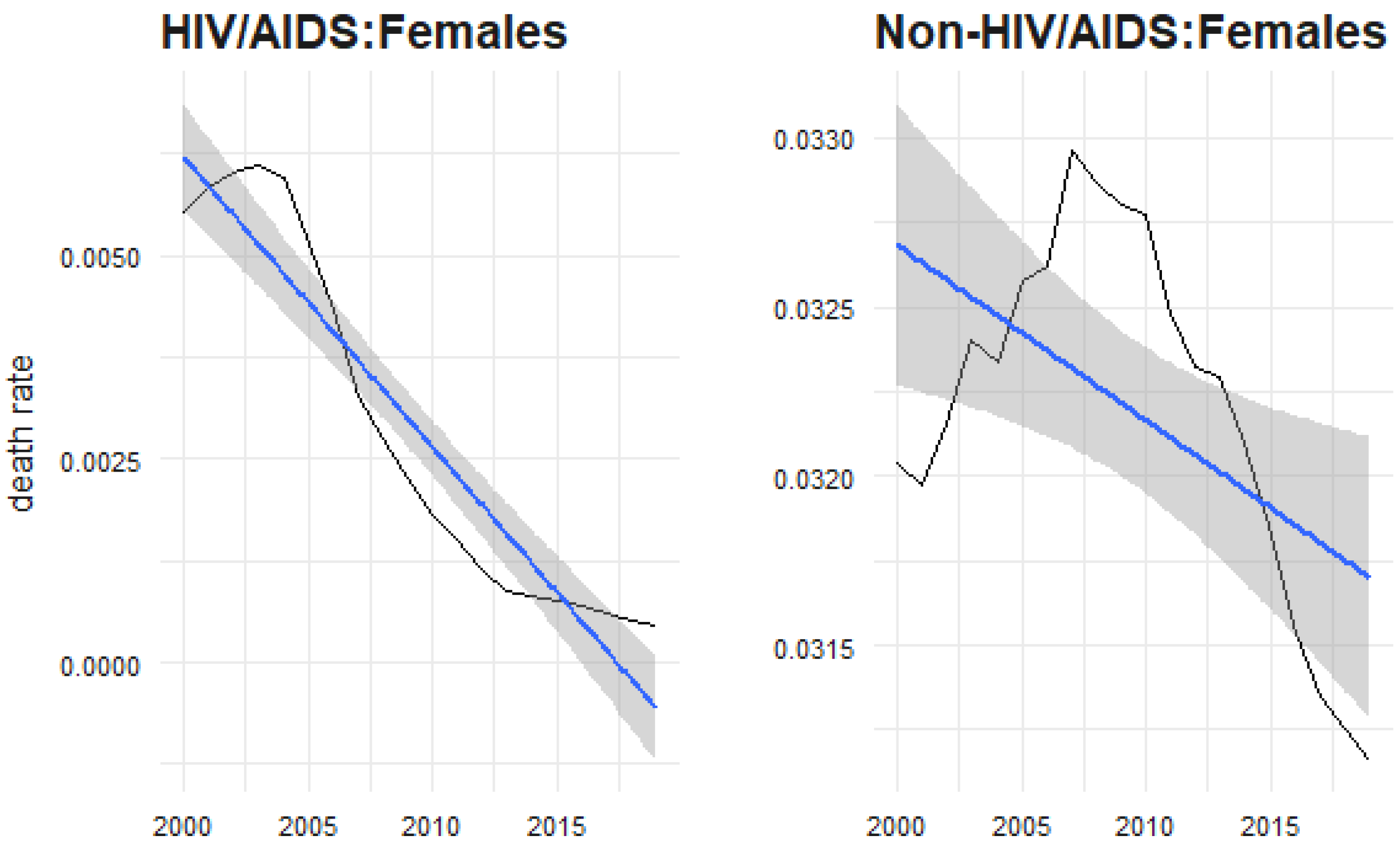
Figure 1 and Figure 2 display the elimination of HIV/AIDS causes of death from the aggregate causes of death over time for both males and females. It is evident that there has been a consistent reduction in mortality rates across the years for both males and females. The fitted abline() indicates a steep declining trend for both HIV/AIDS and non-HIV/AIDS causes of death. This result could suggest the existence of a positive correlation between these two variables. It is interesting to note a higher variability for the non-HIV/AIDS female rates.

4.2. All Causes of Death Distribution with and without HIV/AIDS in Terms of Age

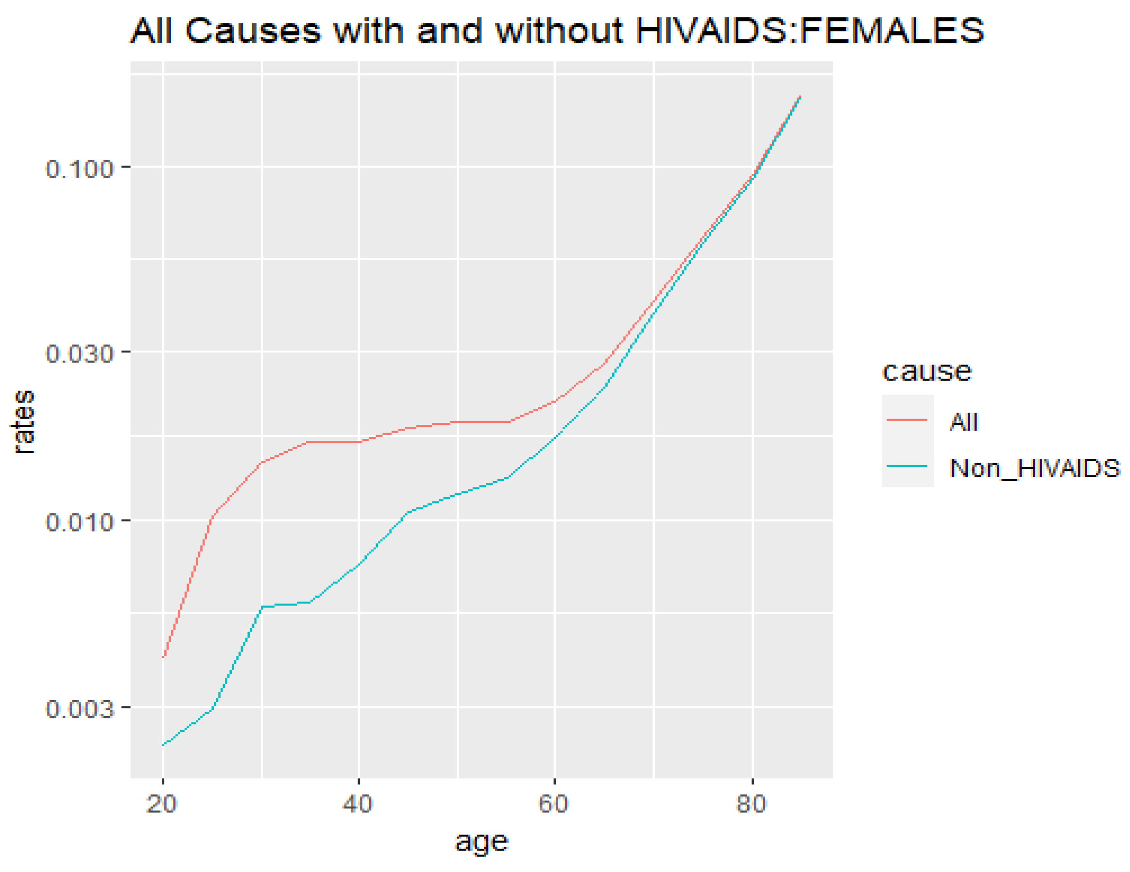
The distribution based on age for males and females is presented in Figure 3 and Figure 4. Firstly, the death rates show a positive correlation with age, that is, the death rates increase with age, which confirms the assumption of the human mortality pattern. Secondly, all causes death rates without HIV/AIDS are lower than all causes to a large extent across all ages, both for males and females; however, we observe there is a significant difference for the younger ages (20 to 50 years) as compared to the older ages. Lastly, it is again seen that the females display a greater difference between the two causes of death. This result explains the impact of HIV/AIDS on the younger population as compared to the older population and also in terms of gender because it seems females are adversely affected by HIV/AIDS as compared to males.

4.3. Joint Distribution for Non-HIV/AIDS against HIV/AIDS Death Rates for Males and Females

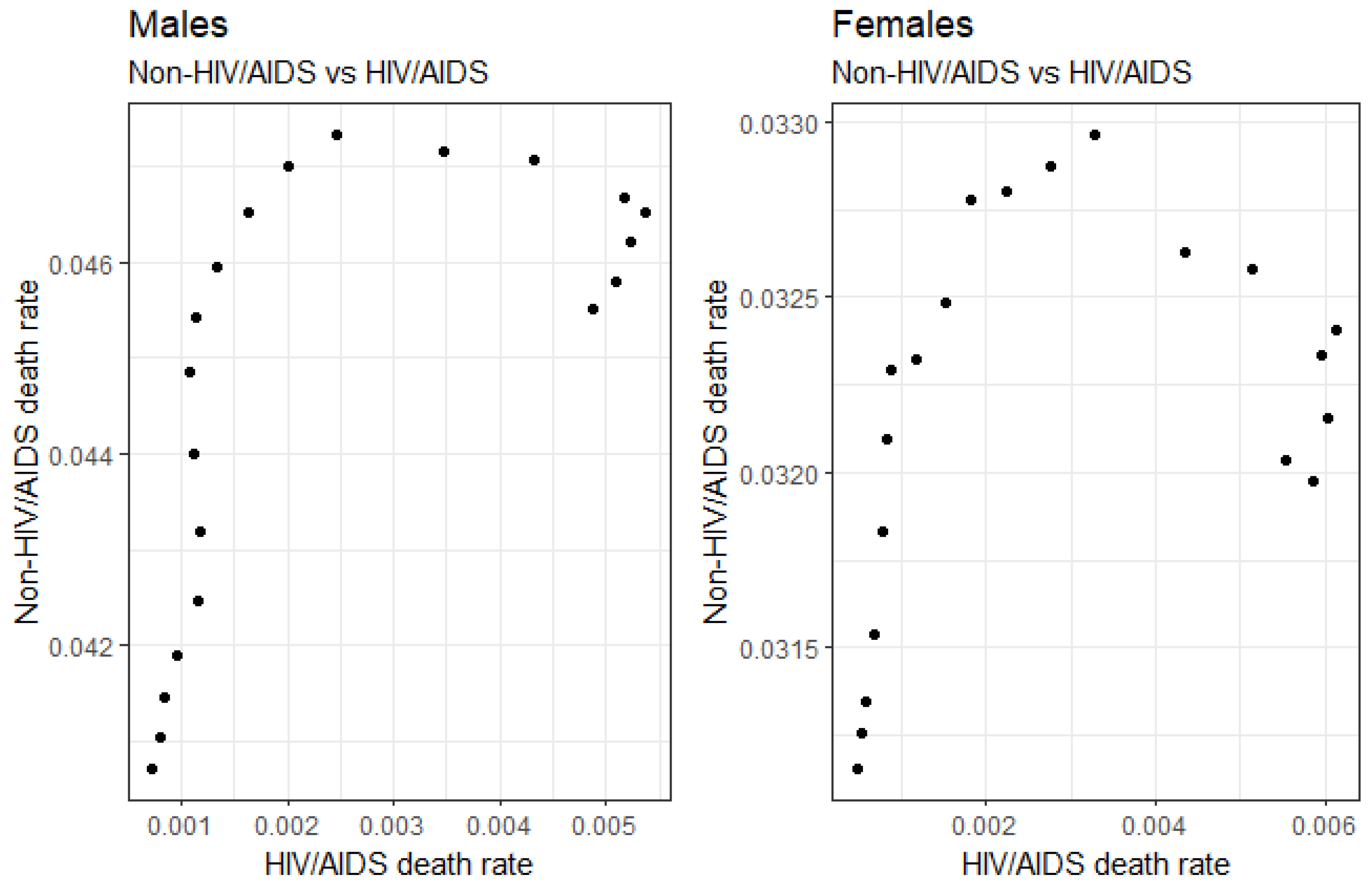
Figure 5 presents the joint distribution of HIV/AIDS and non-HIV/AIDS death rates for males and females. It is a bivariate pair plot of these two causes aged over 20 years running from 2000 to 2019. Despite limited data points, we can observe a positive correlation between these two causes of death within each gender. It is, however, evident that the relationship between this pair is asymmetric and non-linear in structure. Additionally, the female case is observed to be more erratic as compared to its male counterpart. The correlation structure observed by these exploratory results suggests a positive relationship between these two categorized causes of death with both time, age, and gender; however, it is critical to note that we have treated these two categorized causes of death as independent of each other. In reality, this is not the case. To overcome this challenge, a dependency model will first be implemented because a trivial correlation procedure will not fully explain this phenomenon. Therefore, applying a copula structure that caters to dependent causes of death may help better understand the dependency level of the specific causes of death based on age, gender, and time.

4.4. Marginal Distributions for HIV/AIDS and Non-HIV/AIDS for Males and Females

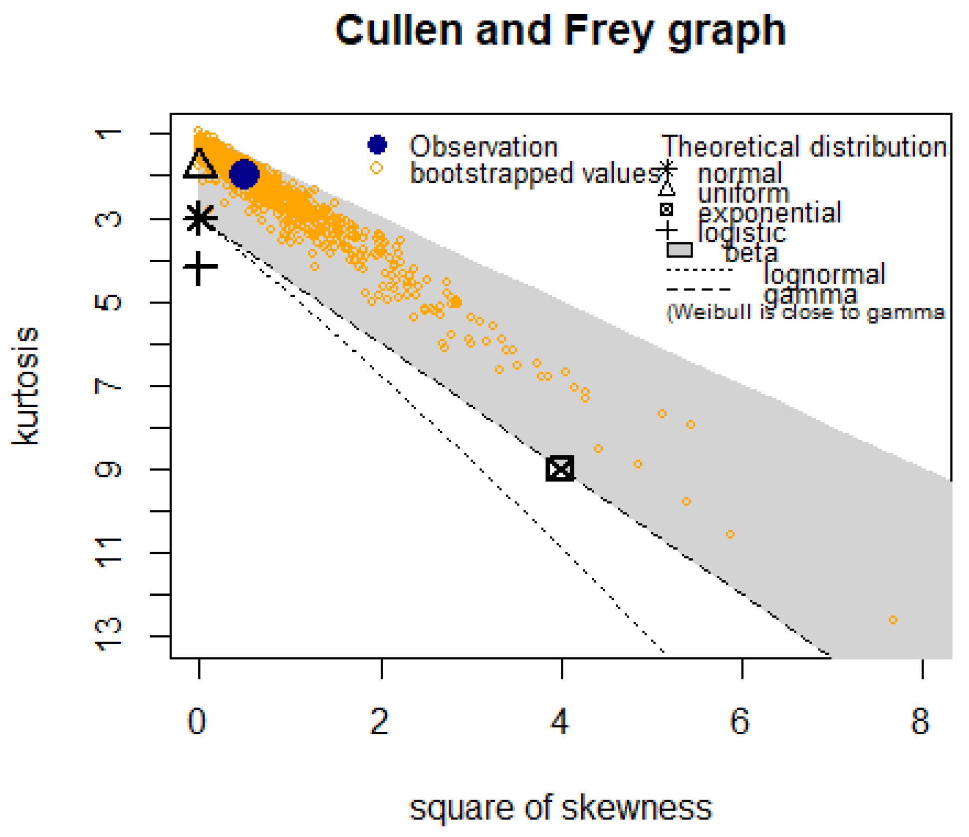
Prior to determining the copula structure, it is prudent first to determine the individual univariate distributions of the two variables. This is because a copula structure is basically a joint multivariate representation of two marginal distributions and their copula. In our case, the two univariate distributions are the non-HIV/AIDS and HIV/AIDS causes of death. Determination of these two distributions is not a trivial matter, and thus a visual and estimation approach will be undertaken. Using the fitdistrplus package in R (Delignette-Muller and Dutang 2015), we achieve both objectives. The output will entail the Cullen and Frey graphs together with the fitted marginals using the maximum likelihood estimation method. The procedure observes from the data the level of kurtosis and skewness and then estimates possible theoretical univariate distributions. For instance, the normal, uniform, exponential, logistic, beta, lognormal, and gamma distributions are potential marginal (univariate distribution) selections. As shown in Figure 6, the estimated marginal distribution for HIV/AIDS for males tends to be a uniform or beta distribution. Similarly, for females, the same is confirmed for HIV/AIDS, as seen in Figure 7. On the other hand, Figure 8 and Figure 9 show the estimated marginal distributions for non-HIV/AIDS for both males and females. As demonstrated by these two graphs, the uniform and beta distributions gave the closest fits for the males and the uniform, beta, and normal distributions for the females.

4.5. Bivariate Copula Analysis

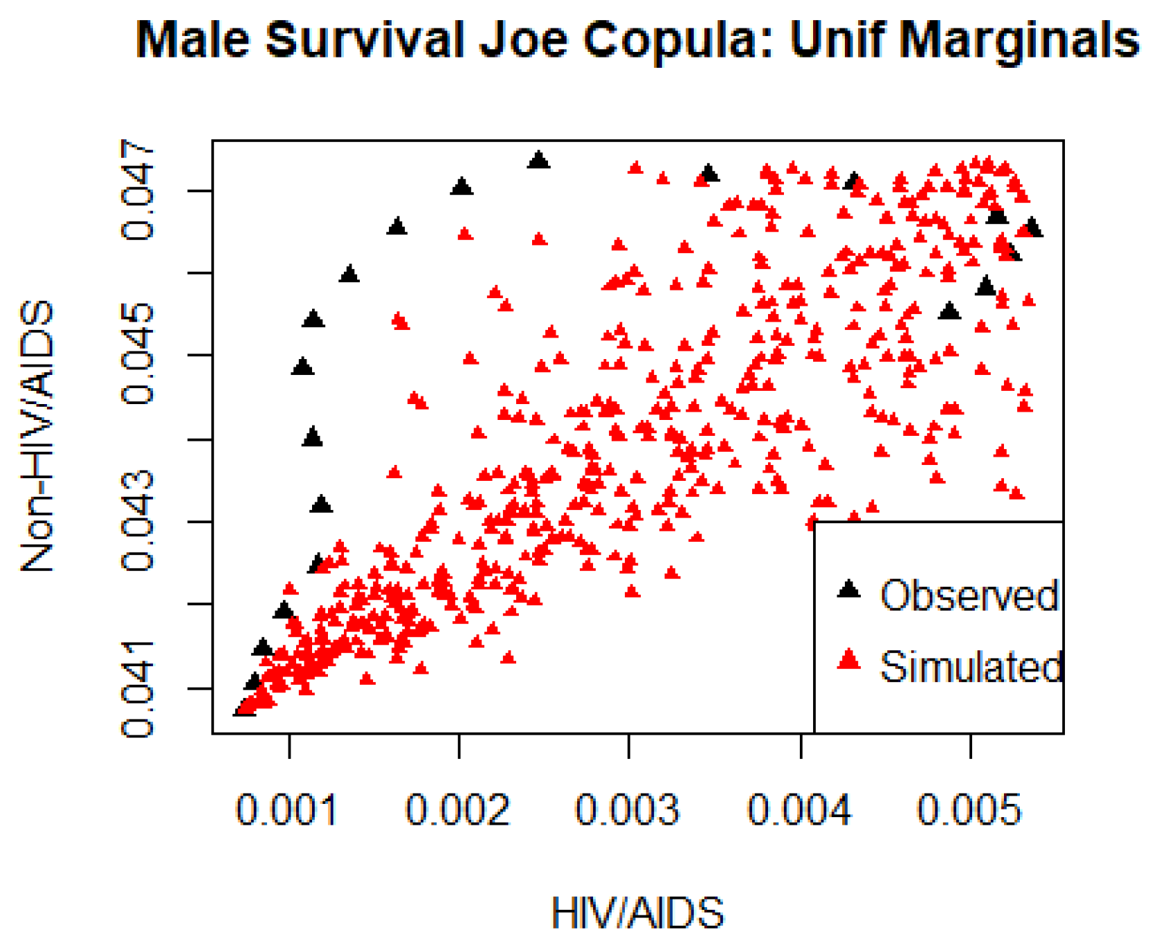
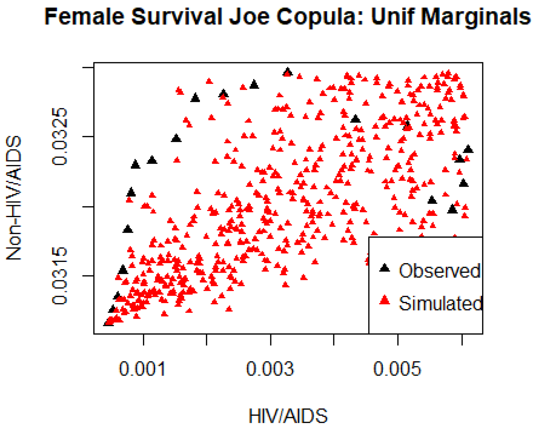
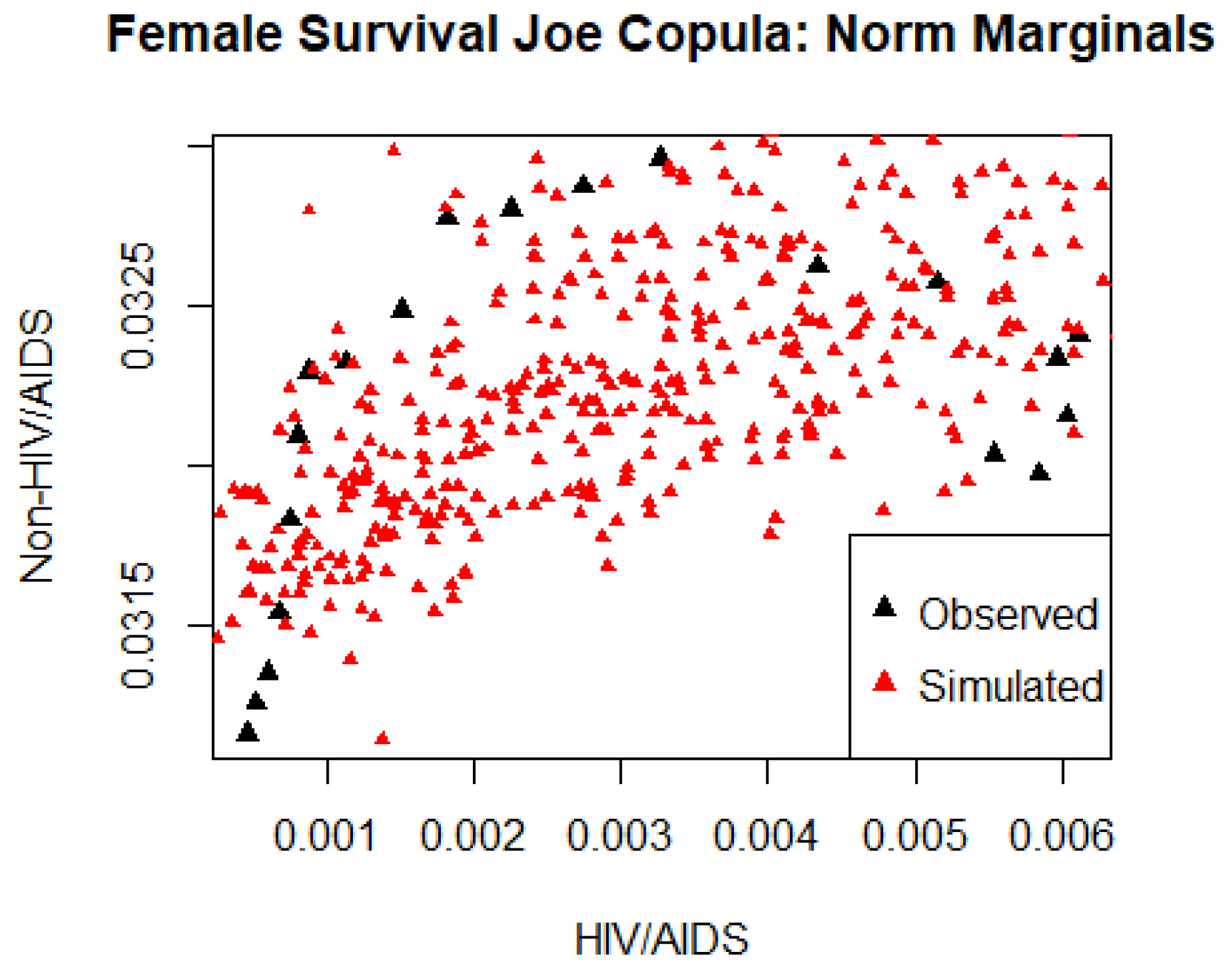
Using the proposed marginals for males (uniform and beta) and females (uniform, beta, and normal), a bivariate copula analysis was performed using the vineCopula package in R, which entailed fitting all the proposed bivariate copula structures as listed in Table 1. The results for the males and females were thus presented in

Table 3. Model selection results for males and females.

	Males			Females
Family Code and Name	logLik	AIC	BIC	logLik	AIC	BIC
0 = independence copula	0	0	0	0	0	0
1 = Gaussian copula	7.84	13.69	−12.69	3.54	−5.08	−4.08
2 = Student t copula (t-copula)	7.78	−11.56	−9.57	3.48	−2.96	−0.96
3 = Clayton copula	14.62	−27.23	−26.23	8.68	−15.36	−14.36
4 = Gumbel copula	4.6	−7.21	−6.21	1.41	−0.82	0.17
5 = Frank copula	7.73	−13.45	−12.45	2.97	−3.93	−2.94
6 = Joe copula	2.03	−2.05	−1.06	0.16	1.69	2.68
7 = BB1 copula	14.61	−25.22	−23.23	8.67	−13.35	−11.36
8 = BB6 copula	4.6	−5.2	−3.21	1.41	1.18	3.17
9 = BB7 copula	14.7	−25.4	−23.41	8.68	−13.36	−11.37
10 = BB8 copula	5.58	−7.16	−5.17	2.13	−0.25	1.74
13 = rotated Clayton copula (180 degrees; survival Clayton)	2.86	−3.73	−2.73	0.63	0.73	1.73
14 = rotated Gumbel copula (180 degrees; survival Gumbel)	10.83	−19.67	−18.67	5.87	−9.74	−8.74
16 = rotated Joe copula (180 degrees; survival Joe’)	14.72	−27.43	−26.44	9.13	−16.25	−15.26
17 = rotated BB1 copula (180 degrees; survival BB1)	10.83	−17.66	−15.66	5.86	−7.73	−5.74
18 = rotated BB6 copula (180 degrees; survival BB6)	14.72	−25.43	−23.44	9.12	−14.25	−12.26
19 = rotated BB7 copula (180 degrees; survival BB7)	14.72	−25.43	−23.44	9.13	−14.25	−12.26
20 = rotated BB8 copula (180 degrees; survival BB8)	14.72	−25.43	−23.44	9.13	−14.25	−12.26
104 = Tawn type 1 copula	4.2	−4.39	−2.4	1.87	0.25	2.24
114 = rotated Tawn type 1 copula (180 degrees)	10.1	−16.2	−14.21	4.56	−5.13	−3.14
204 = Tawn type 2 copula	4.11	−4.21	−2.22	0.99	2.03	4.02
214 = rotated Tawn type 2 copula (180 degrees)	10.6	−17.21	−15.22	7.51	−11.03	−9.03

. The rotated Joe copula (180 degrees; survival Joe) was observed to be the fitted copula structure for the males and females. The optimal selection is seen to be the minimal AIC and BIC and maximum log-likelihood as expected. The parameters achieved for males are Survival Joe (par = 4.77, tau = 0.66) while those for females are Survival Joe (par = 3.29, tau = 0.55).

The observed correlation structure for the males is higher than that of the females; this is presented by a Kendall’s tau of 0.67 against 0.55, respectively. This lower dependency level confirms the evidence of the erratic nature of the relationship between HIV/AIDS and non-HIV/AIDS for females, as seen in Figure 4 and Figure 5. Additionally, the selected marginal distributions are also identified as ideal based on the results in

Table 4. Correlation structure of the bivariate pair HIVAIDS and non-HIVAIDS for males.

Marginals	Pearson Linear Correlation Coefficient	Kendall’s Tau = 0.66
Assuming Independence	0.6417682	0.6
Beta	0.7215273	0.6687808
Uniform	0.8325042	0.6503343

and

Table 5. Correlation structure of the bivariate pair HIVAIDS and non-HIVAIDS for females.

Marginals	Pearson Linear Correlation Coefficient	Kendall’s Tau = 0.55
Assuming Independence	0.3879891	0.4315789
Beta	0.5933727	0.5522082
Uniform	0.7142036	0.5313874
Normal	0.7361025	0.54

for males and females, respectively. It was noted that the beta marginals were suitable for both males and females. Visually, Figure 10, Figure 11, Figure 12, Figure 13 and Figure 14 confirm these results after 500 simulations.

4.6. Independence versus Dependence Assumption

These results establish the fact that treating causes of death independently may lead to erroneous conclusions. A rank-based dependence measure would observe that the correlation structure between HIV/AIDS and non-HIV/AIDS is 0.6 and 0.43 for males and females, respectively, and 0.64 and 0.39 based on a Pearson linear correlation coefficient, as shown in Table 4 and Table 5. The proximity implies that these two dependence measures are generally similar. According to Kendall’s tau, the actual measure of concordance between the two causes of death is 0.669 for males and 0.552 for females. Concordant pairs mean that higher rates of one variable are correlated with the higher rates of the other pair, while discordant pairs signify the opposite. Kendall’s tau values close to zero means that the dependence is low or even that the variables are independent; conversely, if they are close to one, then this pair is dependent.

4.7. Application of Cause-Specific Mortality Models to the Sensitivity to Life Expectancy

We apply the findings of this approach to the Kenyan mortality period life table for the year 2019 as an example. The construction of the life table and the cause-eliminated life table will follow the approach of (Arias et al. 2019; Keyfitz et al. 1972; Chiang 1968), and thus the life expectancy quantity will be obtained as given in Section 3 of this study.

4.8. Life Expectancy Gain/Loss Analysis

Scenarios from simulating the obtained copula structure would aid in fitting the two causes. The determined copulas for males and females were applied and adjusted to the constructed table and the life expectancy at age 20, $e_{20}$, observed for all-cause mortality, non-HIV/AIDS cause mortality assuming independence, and non-HIV/AIDS cause mortality allowing dependence. The results are given in

Table 6. Life expectancy gain/loss analysis for males.

	2019				2010				2000
Age (x)	ex(All Cause)	ex(Non-HIVAIDS) Independence	ex(Non-HIVAIDS) Dependence	Gain/ (Loss)	ex(All Cause)	ex(Non-HIVAIDS) Independence	ex(Non-HIVAIDS) Dependence	Gain/ (Loss)	ex(All Cause)	ex(Non-HIVAIDS) Independence	ex(Non-HIVAIDS) Dependence	Gain/(Loss)
20	44.0	44.9	44.6	−0.3	40.4	42.0	41.0	−1.0	36.1	41.8	37.4	−4.4
25	43.1	44.0	43.7	−0.3	39.4	41.1	40.1	−1.0	35.2	40.9	36.4	−4.5
30	39.5	40.3	40.1	−0.2	35.9	37.5	36.5	−1.0	31.8	37.2	33.0	−4.2
35	35.1	35.8	35.6	−0.2	31.7	33.1	32.3	−0.8	28.2	32.8	29.4	−3.4
40	30.8	31.5	31.4	−0.1	27.9	29.0	28.5	−0.5	25.4	28.8	26.5	−2.3
45	26.9	27.4	27.4	0	24.4	25.2	25.0	−0.2	23.0	25.4	24.0	−1.4
50	23.1	23.5	23.6	0.1	21.3	21.7	21.8	0.1	20.6	22.1	21.4	−0.7
55	19.6	19.8	20.0	0.2	18.2	18.5	18.6	0.1	17.7	18.7	18.5	−0.2
60	16.2	16.4	16.6	0.2	15.1	15.3	15.5	0.2	14.8	15.3	15.5	0.2
65	13.2	13.2	13.5	0.3	12.3	12.4	12.6	0.2	12.0	12.3	12.6	0.3
70	10.3	10.4	10.6	0.2	9.7	9.7	9.9	0.2	9.5	9.7	10.0	0.3
75	7.8	7.8	8.0	0.2	7.4	7.4	7.6	0.2	7.3	7.4	7.6	0.2
80	5.5	5.5	5.6	0.1	5.2	5.2	5.4	0.2	5.3	5.3	5.5	0.2
85+	3.1	3.1	3.2	0.1	3.1	3.1	3.1	0	3.1	3.1	3.2	0.1

and

Table 7. Life expectancy gain/loss analysis for females.

	2019				2010				2000
Age (x)	ex(All Cause)	ex(Non-HIVAIDS) Independence	ex(Non-HIVAIDS) Dependence	Gain/ (Loss)	ex(All Cause)	ex(Non-HIVAIDS) Independence	ex(Non-HIVAIDS) Dependence	Gain/ (Loss)	ex(All Cause)	ex(Non-HIVAIDS) Independence	ex(Non-HIVAIDS) Dependence	Gain/(Loss)
20	48.0	48.7	48.9	0.2	43.6	46.5	44.7	−2.2	37.8	45.6	39.1	−6.5
25	47.1	47.7	48.0	0.3	42.7	45.5	43.8	−1.7	36.9	44.7	38.3	−6.4
30	43.4	44.0	44.3	0.3	39.3	42.0	40.4	−1.6	34.4	41.2	35.7	−5.5
35	39.0	39.6	39.9	0.3	35.5	37.8	36.6	−1.2	31.8	37.3	33.0	−4.3
40	34.8	35.2	35.6	0.4	32.1	33.7	33.1	−0.6	29.4	33.3	30.4	−2.9
45	30.7	31.1	31.5	0.4	28.8	29.8	29.7	−0.1	26.7	29.5	27.6	−1.9
50	26.8	27.0	27.5	0.5	25.5	26.1	26.3	0.2	24.0	26.0	24.8	−1.2
55	22.9	23.0	23.5	0.5	22.0	22.4	22.7	0.3	21.1	22.4	21.9	−0.5
60	19.1	19.2	19.6	0.4	18.5	18.7	19.1	0.4	18.0	18.8	18.6	−0.2
65	15.4	15.4	15.9	0.5	15.0	15.1	15.5	0.4	14.8	15.3	15.3	0
70	11.9	12.0	12.4	0.4	11.7	11.8	12.1	0.3	11.6	11.9	12.1	0.2
75	8.9	8.9	9.2	0.3	8.7	8.8	9.1	0.3	8.8	8.9	9.1	0.2
80	6.1	6.1	6.3	0.2	6.0	6.0	6.3	0.3	6.1	6.2	6.4	0.2
85+	3.4	3.4	3.5	0.1	3.4	3.4	3.5	0.1	3.5	3.5	3.6	0.1

.

4.9. All-Cause Mortality

It is evident that the life expectancy for all-cause mortality has had a consistent increase across the years 2000, 2010, and 2010, as expected for males and females. This is due to the general decline in mortality attributed across the years from 2000 to 2019.

4.10. Non-HIV/AIDS Mortality (Assuming Independence and Allowing Dependence)

Eliminating HIV/AIDS from the causes of death in the early years, such as the year 2000, has the greatest impact because it was during this year that mortality rates were at their highest and life expectancies were at their lowest for males and females. This scenario is evident for both the independence and dependence cases; however, there exist significant differences between the two approaches across years, age, and gender. Based on years, there is a consistent reduction in losses across the years probably due to the fading effect of risks posed by HIV/AIDS. With regard to age, life expectancy losses are experienced in younger years as compared to older ages, as corroborated by Nall et al. (2019). This could be due to two reasons. Fewer data is available at advanced ages, and HIV/AIDS risk is highly prevalent among the young. Based on gender, females experienced the highest losses as compared to males due to the fact that prevalent due to HIV/AIDS is highest among the female population (Sia et al. 2014). Actuaries make adjustments to the life table based on historical data, and if they are to assume independence, then one may overestimate or underestimate the effect of HIV/AIDS on the life table. Using copulas, one may make adjustments to the actual correlation structure of the causes of death and thus quantify its change to the life tables

4.11. Limitation of the Study

The study used 20-year historical mortality data, which is generally insufficient in the majority of mortality studies; however, the dynamic nature of mortality due to mortality shocks would enable this approach to be plausible and be an alternative approach. Furthermore, the application of this model to life tables did not consider smoothing of the mortality rates, which is a common practice in life table construction.

5. Conclusions and Further Work

The aim of the research was to determine an appropriate bivariate copula structure that would fit HIV/AIDS cause of death and non-HIV/AIDS cause of death for both males and females aged 20 and above. It was determined that the Survival Joe copulas were suitable to quantify the dependence structure of HIV/AIDS and non-HIV/AIDS for females and males, respectively. The impact of the causes of death on a life table and specifically life expectancy was measured by the use of this copula where indolence and dependence scenarios were simulated. This dependence model is an advance over the correlation approach because it gives a deeper understanding of the relationship between variables, specifically causes of death. Actuaries may alternatively implement the copula approach so as to quantify the inherent risk and as a way to understand the mortality and longevity risk caused by HIV/AIDS or a specific cause of death.

Further work would entail incorporating trends that would be based on the future development of the cause of death and even extending the two-dimensional case where two or more cases are observed.

References

1. Aas, Kjersti, Claudia Czado, Arnoldo Frigessi, and Henrik Bakken. 2009. Pair-Copula Constructions of Multiple Dependence. Insurance: Mathematics and Economics 44: 182–98. [Google Scholar] [CrossRef]
2. Alai, Daniel H., Severine Gaille, and Michael Sherris. 2013. Modelling Cause-of-Death Mortality and the Impact of Cause-Elimination. UNSW Australian School of Business Research Paper. Sydney: UNSW Australian School of Business Research. [Google Scholar]
3. Arias, Elizabeth, Jiaquan Xu, and Kenneth D. Kochanek. 2019. United States Life Tables, 2016. Available online: https://www.cdc.gov/nchs/data/nvsr/nvsr68/nvsr68_04-508.pdf (accessed on 20 September 2022).
4. Arnold, Séverine, and Michael Sherris. 2015. Causes-of-Death Mortality: What Do We Know on Their Dependence? North American Actuarial Journal 19: 116–28. [Google Scholar] [CrossRef]
5. Bedford, Tim, and Roger M. Cooke. 2002. Vines—A New Graphical Model for Dependent Random Variables. The Annals of Statistics 30: 1031–68. [Google Scholar] [CrossRef]
6. Beltrán-Sánchez, Hiram, Samuel H. Preston, and Vladimir Canudas-Romo. 2008. An Integrated Approach to Cause-of-Death Analysis: Cause-Deleted Life Tables and Decompositions of Life Expectancy. Demographic Research 19: 1323. [Google Scholar] [CrossRef]
7. Bengtsson, Tommy, and Nico Keilman. 2019. Old and New Perspectives on Mortality Forecasting. Berlin: Springer Nature. [Google Scholar]
8. Bett, Nicholas, Juma Kasozi, and Daniel Ruturwa. 2022. Temporal Clustering of the Causes of Death for Mortality Modelling. Risks 10: 99. [Google Scholar] [CrossRef]
9. Bryant, John, and James J. Dignam. 2004. Semiparametric Models for Cumulative Incidence Functions. Biometrics 60: 182–90. [Google Scholar] [CrossRef]
10. Chiang, Chin Long. 1968. The Life Table and Its Construction. Introduction to Stochastic Processes in Biostatistics, 198–214. [Google Scholar]
11. Delignette-Muller, Marie Laure, and Christophe Dutang. 2015. Fitdistrplus: An R Package for Fitting Distributions. Journal of Statistical Software 64: 1–34. [Google Scholar] [CrossRef]
12. Dissmann, Jeffrey, Eike C. Brechmann, Claudia Czado, and Dorota Kurowicka. 2013. Selecting and Estimating Regular Vine Copulae and Application to Financial Returns. Computational Statistics & Data Analysis 59: 52–69. [Google Scholar]
13. Elandt-Johnson, Regina C. 1976. Conditional Failure Time Distributions under Competing Risk Theory with Dependent Failure Times and Proportional Hazard Rates. Scandinavian Actuarial Journal 1976: 37–51. [Google Scholar] [CrossRef]
14. Engle, Robert F., and Clive W. J. Granger. 1987. Co-Integration and Error Correction: Representation, Estimation, and Testing. Econometrica: Journal of the Econometric Society 1987: 251–76. [Google Scholar] [CrossRef]
15. Fergany, Nader. 1971. On the Human Survivorship Function…-Google Scholar. Available online: https://scholar.google.com/scholar?hl=en&as_sdt=0%2C5&q=Fergany+%281971.+%22On+the+Human+Survivorship+Function+and+Life+Table+Construction%2C%22+Demography8%283%29%3A331-334%29&btnG= (accessed on 20 September 2022).
16. Fréchet, Maurice. 1951. Sur Les Tableaux de Corrélation Dont Les Marges Sont Données. Annal Université Lyon, 3^e serie, Sciences, Section A 14: 53–77. [Google Scholar]
17. Kaishev, Vladimir K., Dimitrina S. Dimitrova, and Steven Haberman. 2007. Modelling the Joint Distribution of Competing Risks Survival Times Using Copula Functions. Insurance: Mathematics and Economics 41: 339–61. [Google Scholar] [CrossRef]
18. Keyfitz, Nathan, Samuel H. Preston, and Robert Schoen. 1972. Inferring Probabilities from Rates: Extension to Multiple Decrement. Scandinavian Actuarial Journal 1972: 1–13. [Google Scholar] [CrossRef]
19. Kjærgaard, Søren, Yunus Emre Ergemen, Malene Kallestrup-Lamb, Jim Oeppen, and Rune Lindahl-Jacobsen. 2019. Forecasting Causes of Death by Using Compositional Data Analysis: The Case of Cancer Deaths. Journal of the Royal Statistical Society: Series C (Applied Statistics) 68: 1351–70. [Google Scholar] [CrossRef]
20. Li, Hong, and Yang Lu. 2018. Modeling Cause-of-Death Mortality Using Hierarchical Archimedean Copula. Scandinavian Actuarial Journal 2019: 1–26. [Google Scholar] [CrossRef]
21. McNeil, Alexander J., Rüdiger Frey, and Paul Embrechts. 2015. Quantitative Risk Management: Concepts, Techniques and Tools-Revised Edition. Princeton: Princeton University Press. [Google Scholar]
22. Mueller, Steve. 2004. Strategically Managing AD&D Risk. Risk Management 51: 40. [Google Scholar]
23. Murphy, Sherry L., Kenneth D. Kochanek, Jiaquan Xu, and Elizabeth Arias. 2021. Mortality in the United States, 2020. Available online: https://stacks.cdc.gov/view/cdc/112079 (accessed on 20 September 2022).
24. Nall, Allison, Tiffany Chenneville, Lindsey M. Rodriguez, and Jennifer L. O’Brien. 2019. Factors Affecting HIV Testing among Youth in Kenya. International Journal of Environmental Research and Public Health 16: 1450. [Google Scholar] [CrossRef]
25. Nelsen, Roger B. 2007. An Introduction to Copulas. Berlin: Springer Science & Business Media. [Google Scholar]
26. Richmond, Douglas R. 2009. Drugs, Sex, and Accidental Death Insurance. Tort Trial & Insurance Practice Law Journal 2009: 57–96. [Google Scholar]
27. Schober, Patrick, Christa Boer, and Lothar A. Schwarte. 2018. Correlation Coefficients: Appropriate Use and Interpretation. Anesthesia & Analgesia 126: 1763–68. [Google Scholar] [CrossRef]
28. Sia, Drissa, Yentéma Onadja, Arijit Nandi, Anne Foro, and Timothy Brewer. 2014. What Lies behind Gender Inequalities in HIV/AIDS in Sub-Saharan African Countries: Evidence from Kenya, Lesotho and Tanzania. Health Policy and Planning 29: 938–49. [Google Scholar] [CrossRef] [PubMed]
29. Sklar, Abe. 1973. Random Variables, Joint Distribution Functions, and Copulas. Kybernetika 9: 449–60. [Google Scholar]
30. Sklar, M. 1959. Fonctions de Repartition an Dimensions et Leurs Marges. Publications de l’Institut de statistique de l’Université de Paris 8: 229–31. [Google Scholar]
31. Stander, Y. S., D. J. Marais, and Ilse Botha. 2013. A Comparison of Cointegration and Copula Asset Allocation Approaches. Studies in Economics and Econometrics 37: 1–28. [Google Scholar] [CrossRef]
32. Stracke, Andrea, and Winfried Heinen. 2020. SOA—Influenza Pandemic: The Impact on an Insured Lives Life Insurance Portfolio. Available online: https://www.soa.org/library/newsletters/the-actuary-magazine/2006/june/pub-influenza-the-impact-on-an-insured-lives-life-insurance-portfolio (accessed on 20 September 2022).
33. Strauss, David J., Pierre J. Vachon, and Robert M. Shavelle. 2005. Estimation of Future Mortality Rates and Life Expectancy in Chronic Medical Conditions. Journal of Insurance Medicine 37: 20–34. [Google Scholar]
Figure 1. HIV/AIDS and non-HIV/AIDS distribution for males over time given by the black line (observed trend plot) and the blue line (fitted abline).
Risks 11 00038 g001
Figure 2. HIV/AIDS and non-HIV/AIDS distribution for females over time given by the black line (observed trend plot) and the blue line (fitted abline).
Risks 11 00038 g002
Figure 3. All causes and non-HIV/AIDS cause of death rates distribution for males against age.
Risks 11 00038 g003
Figure 4. All causes and non-HIV/AIDS cause of death rates distribution for females against age.
Risks 11 00038 g004
Figure 5. Joint distribution for non-HIV/AIDS and HIV/AIDS for males and females.
Risks 11 00038 g005
Figure 6. Estimated marginal distribution for HIV/AIDS for males.
Risks 11 00038 g006
Figure 7. Estimated marginal distribution for HIV/AIDS for females.
Risks 11 00038 g007
Figure 8. Estimated marginal distribution for non-HIV/AIDS for males.
Risks 11 00038 g008
Figure 9. Estimated marginal distribution for non-HIV/AIDS for females.
Risks 11 00038 g009
Figure 10. Uniform marginal distribution for males.
Risks 11 00038 g010
Figure 11. Beta marginal distribution for males.
Risks 11 00038 g011
Figure 12. Uniform marginal distribution for females.
Risks 11 00038 g012
Figure 13. Beta marginal distribution for females.
Risks 11 00038 g013
Figure 14. Normal marginal distribution for females.
Risks 11 00038 g014