A Wavelet Analysis of the Dynamic Connectedness among Oil Prices, Green Bonds, and CO₂ Emissions

Abstract

Wavelet power spectrum (WPS) and wavelet coherence analyses (WCA) are used to examine the co-movements among oil prices, green bonds, and CO₂ emissions on daily data from January 2014 to October 2022. The WPS results show that oil returns exhibit significant volatility at low and medium frequencies, particularly in 2014, 2019–2020, and 2022. Also, the Green Bond Index presents significant volatility at the end of 2019–2020 and the beginning of 2022 at low, medium, and high frequencies. Additionally, CO₂ futures’ returns present high volatility at low and medium frequencies, expressly in 2015–2016, 2018, the end of 2019–2020, and 2022. WCA’s empirical findings reveal (i) that oil returns have a negative impact on the Green Bond Index in the medium term. (ii) There is a strong interdependence between oil prices and CO₂ futures’ returns, in short, medium, and long terms, as inferred from the time–frequency analysis. (iii) There also is evidence of strong short, medium, and long terms co-movements between the Green Bond Index and CO₂ futures’ returns, with the Green Bond Index leading.

1. Introduction

The inclusion of oil prices in the analysis of the environmental context comes from the substitution and income effect caused by any change in the product price relative to its demand function (Barsky and Kilian 2004; Hamilton 1983; Kilian 2009). The substitution effect occurs when goods get cheaper, and this generates incentives to consume more of the cheaper goods and less of the expensive ones. On the other hand, the income effect occurs when the price of the goods falls and the purchasing power increase, causing a result similar to a rise in income. This theory is called the Slutzky-Hicks Theory (Allen 1950). In this way, oil price shocks can affect carbon emissions and green bond issuances through changes in fossil fuel consumption. For instance, the sharp decline in oil prices during 2014–2015 increased carbon emissions due to the relatively more expensive clean energy projects (Kassouri et al. 2022, 2021). In this context, a fall in oil prices obstructs carbon mitigation initiatives as green bonds promote them (Kassouri et al. 2022).

With the implementation of the European Union Emissions Trading System (EU ETS) in January 2005, EU Allowances (EUAs) became a tradeable asset that could be negotiated in organized spot, futures, and options markets (Reboredo 2013). Likewise, in January 2014, the International Capital Markets Association (ICMA) published the Green Bond Principles (GBP) to establish the rules for a bond to be labeled green. Since then, investors have at their disposal information to enable them to discern the environmental benefits of their fixed-income investments against alternative investments (Mejía-Escobar et al. 2021; Reboredo 2018). Thus, green bonds are a well-established sustainable investment instrument that has been gaining popularity among (i) investors, especially environmentally-conscious investors, (ii) companies concerned about climate-related risk exposition and the opportunities of financing their eco-friendly projects, and (iii) governments for the potential influence of green bonds on their climate change policies (Reboredo 2018).

Numerous studies evidence the relationship between (i) oil prices and green bonds (Azhgaliyeva et al. 2022, 2021; Dutta et al. 2021; Lee et al. 2021; Reboredo and Ugolini 2020; Saeed et al. 2021; Su et al. 2022), (ii) oil prices and CO₂ emissions (Alhodiry et al. 2021; Ali et al. 2022; Habib et al. 2021; Maji et al. 2020; Mensah et al. 2019; Mujtaba and Jena 2021; Sadorsky 2009; Wen et al. 2017; Zhang and Zhou 2022; Zou 2018), and (iii) green bonds and CO₂ emissions (Jin et al. 2020; Lichtenberger et al. 2022; Nenonen et al. 2019; Rannou et al. 2021; Ren et al. 2022a; Tiwari et al. 2022; Wang et al. 2022).

However, a knowledge gap has been identified despite all the advances in studying the previously mentioned relationships with other financial assets; just a few recent studies in the current literature have provided an in-depth analysis of the co-movements among the green bonds, CO₂ emissions, and oil prices simultaneously (Li et al. 2022; Marín-Rodríguez et al. 2022b). These two studies provide an important foundation for our paper. Furthermore, by using wavelets, we contribute to the debate on the dependences among green bonds, CO₂ emissions, and oil prices simultaneously, conducting a time-frequency analysis of the dependence among these three variables. Moreover, we emphasize the economic and policy implications of the results obtained. Additionally, we make a novel extension to the existing literature focusing on clean energy stocks and other financial markets.

For example, Li et al. (2022) found that oil price has a negative effect on the Green Bond Index and that carbon prices positively influence the Carbon Efficiency Index in the short and medium term. Additionally, the Green Bond Index positively affects carbon prices in the short and medium term and negatively impacts the Carbon Efficiency Index. In addition, carbon price shocks positively affect the Carbon Efficiency Index in the short and medium term. Furthermore, Marín-Rodríguez et al. (2022b) using Granger Causality and DCC-GARCH methodologies, observed a unidirectional causality running from the Green Bond Index to the Brent oil returns and a unidirectional causality running from the Green Bond Index to the CO₂ futures’ returns and a unidirectional causality running from the Brent oil returns to the CO₂ futures’ returns. Also, their results for DCC-GARCH indicate a positive dynamic correlation between the Brent oil price return and the CO₂ futures’ returns and a negative dynamic correlation between the Green Bond Index concerning the oil return and the CO₂ futures’ returns, presenting a solid correlation in uncertainty periods. Thus, a deeper analysis of this concern will lead to a better comprehension of the evolution and co-movements of these three variables in a global decarbonization scenario.

This research is aimed at quantifying such co-movements identifying their effects on different time periods, and how this relationship varies according to the economic conditions. Thus, this paper makes two substantial contributions to the existing body of knowledge and practice. First, this study is the first to incorporate a scientometric analysis of dynamic co-movements among oil prices, green bonds, and CO₂ emissions with particular emphasis on measuring different time period relationships, limiting the search equation to the existence of co-movements, contagion, or dependence among the variables. Second, it provides new evidence by examining the dynamic relationship among crude oil prices, CO₂ futures’ price, and green bonds using a wavelet coherence approach to determine the effects of oil price shocks on CO₂ emissions and green bonds issuances over different time frequencies: short, middle, and long-term. In addition, this study analyzes whether the correlation changes over different scales in the period studied 2014–2022. Thus, this study’s outcomes can help researchers, managers, policymakers, and decision-makers to understand the importance of the oil price shocks on the design of assets and policies that tend to improve sustainability practices.

The paper’s outline is as follows: Section 2 studies the background and bibliometric analysis of asset market linkages among oil prices, green bonds, and CO₂ emissions. Section 3 presents the data, the descriptive statistics, and the methodologies used. Section 4 analyzes the results. Section 5 discusses the empirical results. Finally, in Section 6, some concluding remarks are offered.

2. Context of the Analysis and Literature Review

2.1. Context of the Analysis

For the selected analysis period, 2014–2022, some different exogenous shocks or crises could have caused rupture or change among the linear relationships of financial assets considered in this study. As a starting point, the financial shocks definition by Beirne and Gieck (2014) will be used. This definition states that they are turbulences in asset markets in advanced and emerging economies that affect other international financial markets. Figure 1 presents the timeline of the main common financial shocks. The first event is the Federal Reserve’s Rate reduction announcement (known as the FED’s Taper Announcement), which caused a fall in the prices of financial assets, an increase in volatility, and a decrease in trade volumes and market liquidity, as well as a rise in a government bond, spreads between the end of May and August 2014 at the height of the market turmoil. Later, the first oil price crisis emerged in 2014 and then in 2016. Subsequently, focusing the analysis on a specific region such as Latin America, several events in the region were affected by protectionist uncertainty in its emerging markets, especially Mexico, due to its strong financial and commercial links with the rest of the world, particularly with the United States. Such uncertainty started with the presidential campaign in the United States when the financial markets reflected the tension during each presidential debate. For example, when investors thought the then-candidate Trump would win, the market would drop; and when candidate Clinton seemed most likely to win, markets rose. This was especially reflected in the fluctuation of the financial markets.

In addition to that scheme, other events have caused imbalances in financial assets, not only in Latin America but also globally, such as the trade war between China and the United States that began in March 2018 after Donald Trump announced the tariff imposition of 50,000 million dollars on Chinese products. In response to those actions, the government of the People’s Republic of China applied tariffs on numerous American products.

A dispute in which the World Trade Organization (WTO) had to intervene to reduce tensions arose. Afterward, the global crisis caused by the COVID-19 virus pandemic (an acronym for coronavirus disease, 2019) occurred. It originated in China in December 2019. After it spread to different countries, on 11 March 2020, it was declared a global pandemic by the World Health Organization (WHO). The virus’s expansion has generated economic and social uncertainty, which has influenced the global financial and economic markets, generating losses. Those are difficult to quantify even today, given that the pandemic has not yet been overcome. Additionally, it is necessary to mention that during this global pandemic, there has been a second crisis in oil prices; The member countries of OPEC (Organization of Petroleum Exporting Countries) have decided to cut production due to the sharp drop in crude oil prices, the decline in demand and the substantial volatility. Finally, the recent Russian invasion of Ukraine on 24 February 2022 is bringing consequences in a range of areas, mainly: (i) humanitarian crisis, (ii) food security crisis, and (iii) energy volatility crisis.

2.2. Literature Review

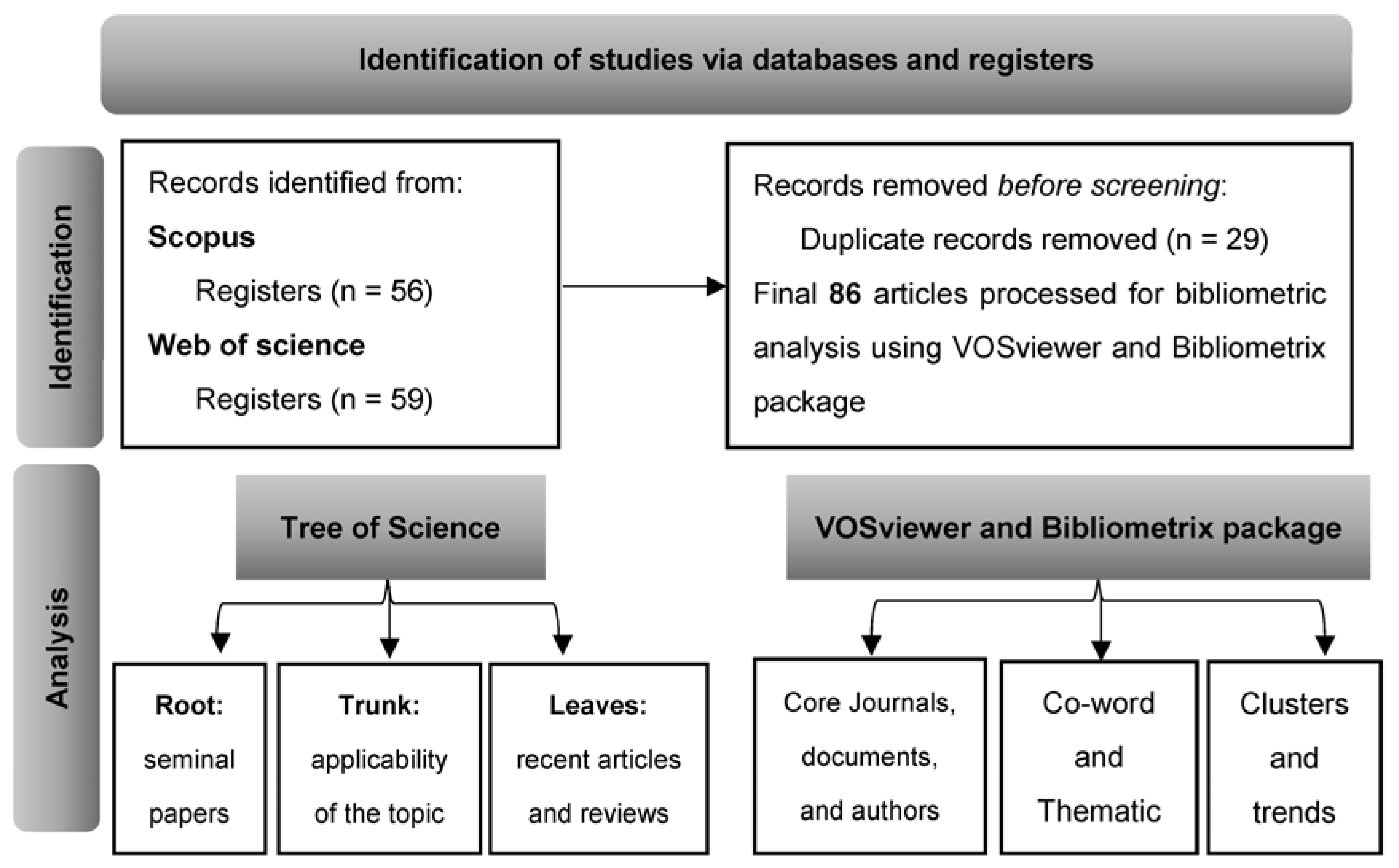
This research includes a scientometric review of the leading studies about the dynamic relationships among oil prices, green bonds, and CO₂ emissions. The documents reviewed were obtained from the Scopus and Web of Science (WoS) bibliographic databases. The research equation was: (TITLE-ABS-KEY (“oil prices*” OR “oil-price*” OR “crude oil” OR “crude-oil”) AND TITLE-ABS-KEY (CO₂ OR “CO₂ emission*” OR “carbon dioxide emission*” OR “carbon emission*” OR “emission* CO₂” OR “green bond*”) AND TITLE-ABS-KEY (“contagion” OR “interdependence*” OR “comovement*” OR “co-movement*” OR “correlation*”)). All the research documents identified were downloaded and ed into the Mendeley Reference Manager for the scientometric analysis. After removing 29 duplicates, we utilized 86 research documents for the scientometric analysis using three tools: (i) the tree of science (Robledo et al. 2014), (ii) the VOSviewer version 1.6.18 (van Eck and Waltman 2017), and (iii) the Bibliometrix package for R (Aria and Cuccurullo 2017). Figure 2 shows the literature search strategy.

As indicated by Robledo et al. (2014), the studies found at the root of the tree of science include seminal articles from the original ones about the dynamic associations among oil prices, green bonds, and CO₂ emissions. For example, studies conducted by (Henriques and Sadorsky 2008; Kumar et al. 2012; Reboredo 2015; Reboredo et al. 2017; Sadorsky 2012) were found in the root, and those papers are the identified seminal studies about the linkages among oil prices and assets related to sustainable finance, such as renewable energy or clean energy stock prices. Refs. (Kumar et al. 2012; Sadorsky 2012) analyze the correlations between clean energy stock prices and oil prices. The findings suggest, for daily data from 2001 to 2010, that stock prices of clean energy companies correlate more highly with technology stock prices than oil prices (Sadorsky 2012). Additionally, based on the weekly observations for the period 2005–2008, Kumar et al. (2012) found that past movements in oil prices explain the indexes of clean energy stocks, stock prices of high technology firms, and interest rates.

Conversely, Robledo et al. (2014) argue that documents in the trunk mainly include the first authors who discovered the applicability and have become references for dynamic associations between oil prices and the financial markets analyzed. Here, documents that study the relationship between energy markets and assets related to sustainable finance can be found, and those used the methodologies of Dynamic Conditional Correlation analysis (DCC-GARCH) or volatility linkages (Dutta et al. 2018; Lin and Chen 2019; Marín-Rodríguez et al. 2022b; Reboredo 2018); and wavelet analysis (Kassouri et al. 2022; Maji et al. 2020). According to Dutta et al. (2018), the results, using daily data from 2009 to 2017, indicate a volatility connection between the emissions and the European Clean Energy Price Indexes. However, this result does not hold for the United States market, suggesting that emissions’ return and volatility shocks are country or region-specific. Lin and Chen (2019), using a daily dataset from 2013 to 2017, found that: (i) There are significant time-varying correlations and a long-run persistence between the Beijing Carbon Emissions Trading (CET) market, the coal market, the stock market of New Energy Companies (NEC), and the coal market; (ii) the new energy stock market has a higher volatility persistence. Additionally, (ii) there is a bi-directional spillover effect between the coal market and the stock market of New Energy Companies.

Finally, the documents in the leaves, according to Robledo et al. (2014), are recent articles and reviews that should condense the analysis of dynamic relationships among oil prices, green bonds, and CO₂ emissions. In the literature review, Marín-Rodríguez et al. (2022a) can be outlined. In the new trends, in the leaves, there are several methodologies identified which have studied the dynamic relationships among energy markets and assets related to sustainable finance, for example, using Time-Varying Parameter Vector Auto Regression (TVP-VAR) (Li et al. 2022), wavelet analysis (Bouoiyour et al. 2023; Kassouri et al. 2022; Luo et al. 2022; Maghyereh et al. 2019; Shah et al. 2022; Zhou et al. 2022), DCC-GARCH and its extensions (Dutta et al. 2021; Marín-Rodríguez et al. 2022b), Copula functions (Elie et al. 2019; Naeem et al. 2021a; Wen et al. 2017), time-varying conditional analysis comprising hedging effectiveness and optimal hedge ratios (Gustafsson et al. 2022), and quantile analysis (Ren et al. 2022a, 2022c; Saeed et al. 2021; Zhang and Zhou 2022).

On the other hand, when exploring the existing literature about the dynamic relationship among oil prices, green bonds, and CO₂ emissions using the VOSviewer, the research pointed out that the most used keywords for this type of analysis are: (1) energy markets, (2) oil prices, (3) CO₂ emissions, and (4) economic analysis. The results of the analyses are presented in Figure 3.

Furthermore, during the revision through the Bibliometrix package for R applying on author keyword analysis, which offers information about research trends from the researchers’ points of view (Garfield 1970), the results indicate that the most prominent research areas are COVID-19 (2022), green bonds (2020–2021), oil prices (2016–2022), and CO₂ emissions (2019–2022). On the other hand, implementing the analysis on the keywords plus, which are terms extracted from titles or abstracts (Aria and Cuccurullo 2017), the findings reveal that the leading research areas are wavelet analysis and COVID-19 (2022), China (2020–2022), oil prices, CO₂ emissions, forecasting (2019–2021), and investments (2020–2022).

Thus, the relationships among oil prices, green bonds, and CO₂ emissions can be classified into these two major trends provided by (i) the authors’ keywords and (ii) keywords plus. The first trend (Figure 3a) delves into the bonds among these three variables, including the effects of the COVID-19 disease (Li et al. 2022; Marín-Rodríguez et al. 2022b). In this trend, the keywords COVID-19, green bonds, oil prices, and CO₂ emissions are precisely leading the trend topics. This result is according to the studies in the leaves of the Tree of Science. Additionally, in this first trend, the documents that study the impacts of the COVID-19 on the green bonds markets can be included (Liu 2022; Naeem et al. 2021b; Rao et al. 2022; Tiwari et al. 2022, 2021), as well as CO₂ emissions (Agboola et al. 2021; Balsalobre-Lorente et al. 2020; Dong et al. 2022; Shah et al. 2022; Tiwari et al. 2022), and oil prices (Alshdadi et al. 2022; Ghorbali et al. 2022; Habib et al. 2021; Ozturk and Cavdar 2021; Ren et al. 2021; Zhou et al. 2022). The findings suggest that the COVID-19 pandemic shock caused huge fluctuations and negative returns in green bond markets (Liu 2022). Furthermore, the contraction of economic growth since the beginning of the COVID-19 pandemic produced a reduction in CO₂ emissions (Agboola et al. 2021). Finally, the results also indicate that COVID-19 negatively impacted crude oil prices, which contributed to the reduction of CO₂ emissions during the pandemic period (Habib et al. 2021).

The second trend (Figure 3b) analyzes the interlinkages between oil prices and CO₂ emissions. For example, (Ali et al. 2022; Alkathery and Chaudhuri 2021; Apergis and Payne 2015; Royal et al. 2022; Sadorsky 2009; Zaghdoudi 2017) analyze the co-movements among oil prices, CO₂ emissions, and renewable energy. The findings suggest that renewable energy improves environmental quality in both the short and long run; an increase in oil prices causes a decrease in CO₂ emissions and has an important effect on economic growth. Additionally, other documents within this trend study the effects of oil price shocks on CO₂ emissions (Bassey 2015; Habib et al. 2021; Husaini et al. 2021; Maji et al. 2020; Ren et al. 2022b; Wei et al. 2022). Their results indicate that there is a negative relationship between oil price shocks and CO₂ emissions; higher oil prices can mitigate CO₂ emissions, while lower oil prices can increase sectoral CO₂ emissions. Besides, COVID-19 affects crude oil prices, the major contributor to the reduction of CO₂ emissions during the pandemic period. In this trend, the keywords COVID-19, wavelets, China, oil prices, CO₂ emissions, and forecasting are the foremost trend topics.

Finally, based on the scientometric analysis of the main studies on the dynamic co-movements among oil prices, CO₂ emissions, and green bonds conducted by Marín-Rodríguez et al. (2022a) on the dynamic co-movements among oil prices and financial markets (including energy markets and assets related to sustainable finance), the findings indicate that the most promising areas for further research in this field are represented by co-movement, copula, wavelet, dynamic correlation, and volatility analysis. Furthermore, the authors indicate that energy markets and assets related to sustainable finance emerge as crucial trends in exploring dynamic co-movements of oil prices. Additionally, as we mentioned before, Marín-Rodríguez et al. (2022b) make a previous application to the analysis of the dynamic co-movements among oil prices, CO₂ emissions, and green bonds using Granger causality and DCC-GARCH methodologies. Thus, in line with these two documents and the results of the present literature review, this study attempts to make a deeper analysis considering a time-frequency analysis (using wavelets methodology) that searches for the connection among the three variables studied in the short, medium, and long term.

3. Methodology

3.1. The Dataset

The dataset consists of daily closing prices of Brent oil prices, green bonds, and CO₂ emissions (

Table 1. List of variables.

Variable	Ticker	Description
Oil Brent price	CO1 Comdty	Generic 1st Crude Oil, Brent
Green Bond Index	GBEUTREU Index	Bloomberg MSCI Euro Green Bond Index Total Return Index Value Unhedged
CO2 futures price	MO1 Comdty	CO2 futures price, Euros per ton

Source: Authors’ own research using Bloomberg.

). Our sampling period spans from 1 January 2014 to 3 October 2022, including 2290 daily observations. The starting date of the sample is determined by the availability of the Green Bond Index data. All data were gathered from Bloomberg. Futures’ prices of CO₂ emissions (MO1 Comdty), according to Reboredo (2013) and Rittler (2012) were used. They indicate that the futures market leads the price training process by first locating information and then transferring it to the spot market. Furthermore, the Bloomberg MSCI Green Bond Index (GBEUTREU Index) is a Euro fixed-income benchmark to fund projects with direct environmental benefits. This index incorporates Euro-denominated fixed-income securities, such as treasury, corporate, government-related, and securitized debt. Additionally, the index reflects the performance of Euro-denominated fixed-income securities, including treasury, corporate, government-related, and securitized debt. Furthermore, the Brent oil price (CO1 Comdty) is included as a fundamental component of energy prices.

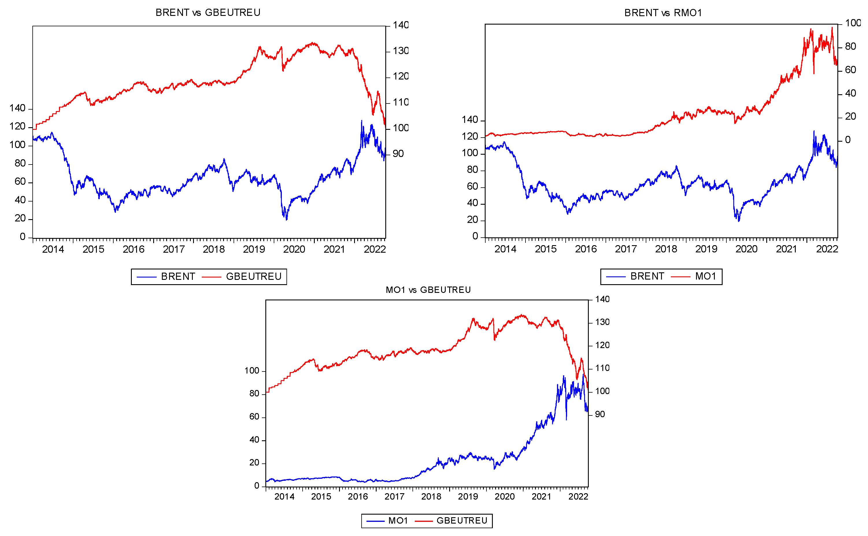
Figure 4 illustrates the temporal dynamics of Brent oil prices, green bonds, and CO₂ emissions by pairs, evidencing that oil prices positively depend on CO₂ futures prices (MO1 Comdty). Still, the dependence is negative with the Green Bond Index (GBEUTREU Index). Furthermore, in recent times the co-movements are increasing between the Green Bond Index (GBEUTREU Index) and CO₂ futures prices (MO1 Comdty), indicating clear graphical evidence of dependence, particularly in 2022.

Table 2. Summary statistics of daily returns.

Index	Mean	Max	Min	Std. Dev.	Skew.	Kurt.	JB	ADF	LBQ (25)	LBQ2 (25)
RBRENT	−0.000063	0.1908	−0.2798	0.0256	−0.982	19.46	26198.4 *	−47.16 *	48.36 [0.003]	836.81 [0]
RGBEUTREU	0.000004	0.0196	−0.0196	0.0027	−0.164	11.13	6315.4 *	−44.18 *	61.73 [0]	1655.0 [0]
RMO1	0.001145	0.162	−0.1944	0.0292	−0.527	7.61	2133.5 *	−50.34 *	38.42 [0.042]	306.21 [0]

Source: Authors’ own research using data from Bloomberg. Notes: This table presents summary statistics of daily returns of Brent oil prices (RBRENT), Green Bond Index (RGBEUTREU), and CO₂ futures’ returns (RMO1). The 1 January 2014—3 October 2022 sample yielded 2290 observations. (*) indicates the rejection of the null hypothesis at the 5% level for both the normality test (via Jarque-Bera) and unit root test [via Augmented Dickey-Fuller (ADF)], the ADF test is conducted with an intercept. LBQ (25) and LBQ2 (25) denote the Ljung–Box Q-statistics for serial correlation in the returns and squared returns series, respectively, computed using 25 lags, with p values reported in square brackets.

depicts descriptive statistics of daily returns of the considered series computed as the first difference of the natural log of the prices or indexes. The average daily returns are close to zero for all series. The standard deviations reveal that green bonds are less volatile than Brent oil prices and CO₂ futures’ prices. All daily returns are negatively biased and exhibit high values for the Kurtosis statistics consistent with heavy-tailed distortions. The Jarque–Bera (JB) test strongly rejects the normality of the unconditional distribution of the return series and the non-stationarity tests [via Augmented Dickey-Fuller (ADF)] (Dickey and Fuller 1979) evidence that all return series are stationary. Finally, the Ljung–Box Q-statistics (LBQ) indicate the presence of a serial correlation in both the return series and the squared return series; it is consistent with the existence of conditional heteroskedasticity effects.

3.2. Wavelet Analysis

The wavelets methodology is one of the mathematical applications that has recently been applied to modeling in several fields, including economics and finance. It allows for the analysis of the time series frequency and time domain simultaneously. This methodology is based on the Fourier Analysis, which focuses on studying frequency domain signals. In this way, wavelets are functions that oscillate as a wave and present fades; that is, they decay. Due to these particularities, this methodology is considered an ideal filter that allows the fragmenting of a signal into different levels of resolution, capturing large and small particularities of the analyzed series. This is known as multi-resolution decomposition using wavelets, which facilitates the decomposition of the original signal into different levels of resolution where each level will necessarily be associated with a specific time scale. The existence of non-stationary phenomena, that is, those presenting variations over time and which do not have a constant mean and/or variance in various disciplines such as geophysics, medicine, statistics, economics, and finance, among others, has expanded the use of wavelets to be ideal for the treatment of this type of series.

Ftiti et al. (2016) indicate that among their advantages, the following stand out: (i) wavelets are a process that breaks down data into different frequency components. This decomposition of different scales facilitates to distinguish of seasonality, structural changes, volatility clusters, and the identification of the local and global dynamic properties of the variables; (ii) Wavelets provide a better alternative for exploring the interconnection between oil and stock markets, as they do not impose parametric constraints on stock market dynamics and oil price fluctuations and (iii) The wavelet process adapts to different characteristics of the time series in general (such as the stock market and oil price series), where the variance is variable over time, and the covariance matrix presents possible structural breaks. This feature helps discriminate between interdependence (long-term co-movement) and contagion (short-term co-movement) in the relationship between oil and financial markets, which will be the subject of the application in this study. However, Dibal et al. (2018) identify weaknesses in the methodology, such as its excessive redundancy, its computational intensity, and the fact that an original signal cannot be perfectly reconstructed from the coefficients estimated by the process.

This research studies the co-movement among oil prices, green bonds, and CO₂ emissions, leading to knowing the linkage across different horizons (i.e., short-medium-and long-term). The wavelet coherency approach by Grinsted et al. (2004) offers this possibility by decomposing the economic relationship into time-frequency components. Furthermore, the wavelet coherency can be applied to bivariate and multivariate contexts, where patterns of covariation and causal relationships among variables across different scales are examined over time (Ahmed 2022). This methodology is similar to the Pearson Bivariate Correlation Coefficient. It measures the degree of co-movement in the time-frequency (location–scale) domain between a pair of time series variables x(t) and y(t) (Singh et al. 2022).

3.2.1. The Continuous Wavelet Transform (CWT)

Thus, the wavelet technique (i) decomposes the return series into time-scale components, and (ii) represents the variability and structure of the stochastic processes on a scale-by-scale basis. The wavelet function is a small wave and can be manipulated (stretched or squeezed over time) to extract the frequency components from a complex signal (Bouri et al. 2020).

The mother wavelet is used to produce small waves. It is expressed as a function of time and scale s as:

$${\psi }_{\tau ,s}\left(t\right)=\frac{1}{\sqrt{s}}\psi \left(\frac{t-\tau }{s}\right)$$

(1)

where $\tau$, s, and $\frac{1}{\sqrt{s}}$ represent the time position (translation parameter), scale (dilation parameter related to frequency) and normalization factor, respectively. The normalization factor ensures that the transformation remains comparable across scales and over time.

The literature provides various wavelets for the time series decomposition depending on the research topic. To examine the wavelet coherence among oil prices, green bonds, and CO₂ emissions, the Morlet Wavelet is used (Morlet et al. 1982). This wavelet provides the best balance between time and frequency localization (Addison 2017). Grinsted et al. (2004) show that the Fourier period for the Morlet wavelet is almost equal to the scale used:

$${\psi }^M\left(t\right)=\frac{1}{{\pi }^{1/4}}{e}^{i{\omega }_{0}t}{e}^{-t^2/2}$$

(2)

where ${\omega }_0$ indicates the central wavelet frequency. Like Bouri et al. (2020), this research used ${\omega }_0$ = 6, as the Morlet wavelet; this central frequency provides good localization between time and frequency.

3.2.2. Wavelet Power Spectrum

The wavelet analysis can be performed using either the continuous wavelet transforms (CWT), or the discrete wavelet transform (DWT). The CWT has several advantages over the DWT. For example, the CWT provides independence to select wavelets according to the length of data, and the redundancy in the CWT makes the interpretation and discovery of patterns or hidden information easier (Aguiar-Conraria and Soares 2011). A continuous wavelet transform $W_x$ of a discrete-time series ($x\left(t\right)$, t = 0, 1, …, n) with respect to $\psi \left(t\right)$ can be represented as:

$$W_x\left(\tau ,s\right)={{\displaystyle \int }}_{-\infty }^{+\infty }x\left(t\right){\psi }_{\tau ,s}^{*}\left(t\right)dt=\frac{1}{\sqrt{s}}{{\displaystyle \int }}_{-\infty }^{+\infty }x\left(t\right){\psi }^{*}\left(\frac{t-\tau }{s}\right)dt$$

(3)

where * denotes the complex conjugate. Notably, the wavelet transform preserves the energy of a time series that can be used to analyze the power spectra. Accordingly, the variance is given by:

$${\Vert x\Vert }^2=\frac{1}{C_{\psi }}{{\displaystyle \int }}_0^{\infty }\left[{{\displaystyle \int }}_{-\infty }^{+\infty }\left|W_x{\left(\tau ,s\right)}^2\right|d\tau \right]\frac{ds}{s^2}$$

(4)

To obtain information about the time series behavior, the wavelet power spectrum (WPS) was used in the present paper,

$$WP{S}_x\left(\tau ,s\right)={\left|W_x\left(\tau ,s\right)\right|}^2$$

(5)

Refs. Hudgins et al. (1993) and Torrence and Compo (1998) define the cross-wavelet power | $W_{xy}\left(\tau ,s\right)$ | of two time series x(t) and y(t) with the continuous transforms $W_x\left(\tau ,s\right)$ and $W_y\left(\tau ,s\right)$ as:

$$W_{xy}\left(\tau ,s\right)=W_x\left(\tau ,s\right).W_y^{*}\left(\tau ,s\right)$$

(6)

3.2.3. Wavelet Coherence

The cross-wavelet power shows the areas of high common power between two time series in the time-frequency space. The wavelet squared coherence between the two times series is given by:

$$R_{xy}^2\left(\tau ,s\right)=\frac{{\left|S\left(s^{-1}{W}_{xy}\left(\tau ,s\right)\right)\right|}^2}{S\left(s^{-1}{\left|W_x\left(\tau ,s\right)\right|}^2\right).S\left(s^{-1}{\left|W_y\left(\tau ,s\right)\right|}^2\right)}$$

(7)

where $R_{xy}^2\left(\tau ,s\right)$ represent the wavelet squared coherency between x(t) and y(t), in other words $R_{xy}^2\left(\tau ,s\right)$ is a direct measure of the contemporaneous correlations between x(t) and y(t) at each point in time and for each frequency. $S(.)$ is a smoothing parameter in scale and time. The value of the wavelet squared coherence $R_{xy}^2\left(\tau ,s\right)$ ranges between zero (no co-movement) and one (high co-movement) can be seen as a scale-specific squared correlation between series. In addition, the wavelet coherence framework allows studying the lead-lag relationship between series while avoiding the squared coherence’s inability to distinguish between the positive and negative relationship between series. Torrence and Webster (1999) and Bloomfield (2013) show that the phase difference depicting the phase relationship between x(t) and y(t) is given by:

$${\varphi }_{xy}\left(\tau ,s\right)=ta{n}^{-1}\frac{\Im \left\{W_{xy}\left(\tau ,s\right)\right\}}{\Re \left\{W_{xy}\left(\tau ,s\right)\right\}},{\varphi }_{x,y}\in \left[-\pi ,\pi \right]$$

(8)

where the parameters $\Im$ and $\Re$ give the imaginary and real parts of the smooth power spectrum, respectively. A zero-degree phase difference reveals the synchronization of x(t) with y(t) at a particular time-frequency. On the wavelet coherence plots, ${\varphi }_{xy}\left(\tau ,s\right)$ is symbolized as black rightward, leftward, upward, and downward arrow signs within areas of statistical significance. When the arrow points to the right (left) suggests that x(t) and y(t) are in phase (out of phase); it means that x(t) and y(t) are positively (negatively) associated, with negligible or no time lag. If the arrow points upwards, the first series leads the other by π/2 (the actual period is based on the specific frequency/scale of the wavelet coherence chart), and the opposite for a downward-pointing arrow. Additionally, for the interpretation of the arrows, following Kirikkaleli and Güngör (2021) arrows pointing up, right-up, or left-down denote that the second variable causes the first variable, while arrows pointing down, right-down, or left-up indicate that the first variable causes the second variable.

The wavelet coherence results are standardly shown on a chart with time and scale (or frequency) on the respective axes and the coherences are represented by a color scale. The color spectrum shows the intensity of the association (co-movement) between the pair of the analyzed series. The warmer colors (red) indicate significant co-movements, while colder colors (blues) signify weak co-movements between the series. In regions beyond the black line cone or the cone of influence, the estimates of wavelet coefficients are statistically insignificant at 5% significance and are not considered.

4. Application and Results

4.1. Unconditional Correlation Analysis

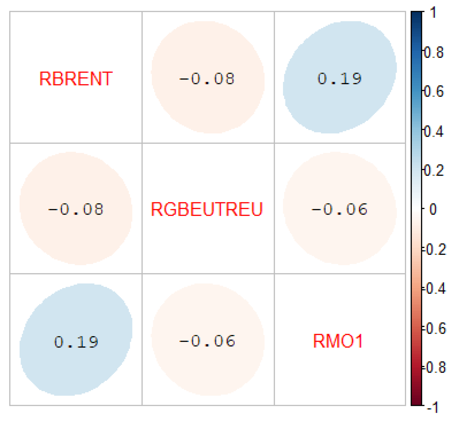
Pairwise correlations across the returns of the variables considered are presented in Figure 5. The correlation of oil price return (RBRENT) with the CO₂ futures’ returns (RMO1) is positive (19%), and the Green Bond Index (GBEUTREU) is negative (−6%). Additionally, the correlation between the CO₂ futures’ returns (RMO1) and the Green Bond Index return (GBEUTREU) is negative too (−8%).

According to the existing literature, it is expected that oil prices and CO₂ emissions have a positive relationship, and their co-movement against the Green Bond Index is in the same sense because an increase in oil prices tends to increase CO₂ emissions (Mahmood et al. 2022; Mahmood and Furqan 2021; Sadorsky 2009; Zheng et al. 2021). Additionally, increasing green bond issuances tends to reduce CO₂ emissions (al Mamun et al. 2022; Fatica and Panzica 2021). For example, the study conducted by al Mamun et al. (2022) shows that green finance significantly reduces carbon emissions in the short and long run by supporting waste and pollution control and improving energy efficiency.

4.2. Wavelet Power Spectrum

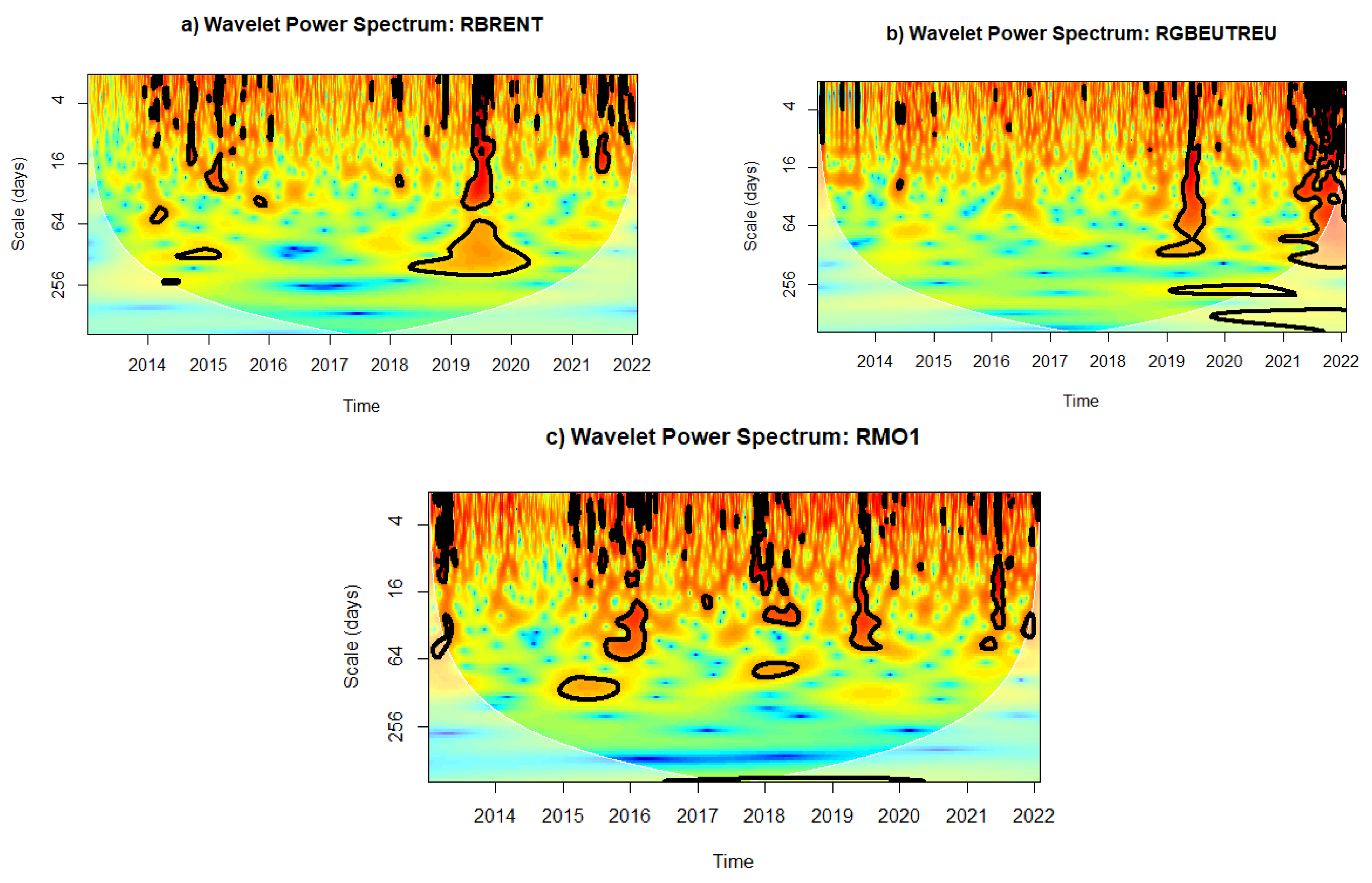
Figure 6 presents the wavelet power spectrum for the Brent oil returns (RBRENT), Green Bond Index (RGBEUTREU), and CO₂ futures’ returns (RMO1) variables, respectively. The Brent oil returns (RBRENT), Figure 6a, appear to show significant volatility at low and medium frequencies, particularly in 2014, the end of 2019–2020, and 2022. This phenomenon is according to the high volatility observed in these periods due to the FED’s Taper Announcement and the first oil prices crisis in 2014, the global COVID-19 pandemic at the end of 2019–2020, and the Russian invasion of Ukraine in February 2022.

The Green Bond Index (RGBEUTREU) behavior, Figure 6b, exhibits significant volatility at the end of 2019–2020 and the beginning of 2022 at low, medium, and high frequencies, which is consistent with the two last events identified previously. For example, in 2019–2020, the issuances of green bonds were extended worldwide. However, in February 2022, the Russian invasion of Ukraine and the subsequent European energy crisis exacerbated post-COVID-19 inflation and impacted the bond market dynamics by increasing interest rates. As a result, high volatility resulted in decreased bond issuance. It is important to note that the Green Bond Principles (GBP) were launched in 2014, its first update occurred in 2015, and the development of this market is constantly changing.

Finally, CO₂ futures’ returns (RMO1), Figure 6c, present high volatility at low and medium frequencies, particularly in 2015–2016, 2018, the end of 2019–2020, and 2022.

4.3. Wavelet Coherence Approach

The wavelet coherence approach is applied to capture the causal relationship between the Brent oil returns (RBRENT), the Green Bond Index (RGBEUTREU), and the CO₂ futures’ returns (RMO1). Figure 7 presents the results from the wavelet coherence. It captures the co-movement of these three variables in the time-frequency space.

Figure 7 and its table depict the wavelet coherence and phase difference and principal results between each pair of times series considered. In the figure, the horizontal axis (x-axis) represents the research period in days, while the vertical axis (y-axis) represents the frequency domain. This study considered five frequency cycles: 1–4, 4–16, 16–64, 64–256, and 256–512 daily bands. The shortest band, which considers 2–4 days, denotes the highest frequency band, and the most extended band includes 256–512 days, the lowest frequency band. For a better comprehension of the results, they include in the short-term (ST), the signals between the 2–4 days and 4–16 bands; medium-term (MT), the signals between the 16–64 days and 64–256 bands; and long-term (LT) the signals in 256–512 days band (see Figure 7 and its table). Located on the right-hand side of each plot, there is the color gradient code of power, where dark blue indicates low power (close to zero), and dark red implies high power (close to one).

Figure 7a shows that wavelet coherence between the Brent oil returns (RBRENT) and the Green Bond Index (RGBEUTREU) from scales 64 to 256 days, down arrows are obtained in 2014, indicating that in the medium-term, the Brent oil returns (RBRENT) significantly affected the Green Bond Index (RGBEUTREU) negatively. However, the direction of the causality changes between 2019–2020 at different frequencies (16–64 and 64–256 days, medium-term and long-term, respectively) since the arrows mostly point right-up, implying a positive relationship and that the Green Bond Index (RGBEUTREU) is an important predictor of the Brent oil returns (RBRENT) in the medium-term and long term for the period between 2019–2020. Finally, in 2021, the Brent oil returns (RBRENT) significantly affected the Green Bond Index (RGBEUTREU) for scales 16–64, and the arrows mostly point left-up, indicating a negative relationship in the medium-term. The summary of the results in the table supports a bi-directional causality relationship between the Brent oil returns (RBRENT) and the Green Bond Index (RGBEUTREU).

Additionally, Figure 7b depicts that wavelet coherence between the Brent oil returns (RBRENT) and CO₂ futures’ returns (RMO1) presents, from scales 4 to 16 days, arrows that point down and left-down in 2014, indicating that in the short term, the CO₂ futures’ returns (RMO1) affected Brent oil returns (RBRENT) significantly with a negative relationship. In 2018, Figure 7b indicates that from scales 4–16 and 64–256, the arrows point right, implying that in the short-term and medium-term, Brent oil returns (RBRENT) influenced the CO₂ futures’ returns (RMO1) with a positive relationship. From 2019 to 2020, Figure 7b shows a change in the direction of the causality for the frequencies 16–64, indicating that in the medium-term CO₂ futures’ returns (RMO1) significantly influenced the Brent oil prices (RBRENT) with a positive relationship. However, for the period between 2019–2020, left-up arrows are obtained for a scale of 16–64, indicating that in the medium-term, the Brent oil returns (RBRENT) significantly affected the CO₂ futures’ returns (RMO1) with a negative relationship. Additionally, for the frequency 64–256 days in the period 2021, the presence of left-down arrows indicates that in the medium-term CO₂ futures’ returns (RMO1) significantly caused the Brent oil prices (RBRENT) with a negative relationship. Finally, for scales 256–512 days, the arrows point right-down, indicating that in the long-term, Brent oil returns (RBRENT) significantly caused the CO₂ futures’ returns (RMO1) with a positive relationship. The summary of the findings in the table validates a bi-directional causality relationship between the Brent oil returns (RBRENT) and CO₂ futures’ returns (RMO1).

Finally, Figure 7c presents the wavelet coherence between CO₂ futures’ returns (RMO1) and Green Bond Index (RGBEUTREU). In 2014, from scales 64 to 256 days, arrows pointed right, denoting that the Green Bond Index (RGBEUTREU) and CO₂ futures’ returns (RMO1) have a positive relationship in the medium-term. But, in 2014, from scales 256–512, arrows point left-down, which indicates that the Green Bond Index (RGBEUTREU) affects the CO₂ futures’ returns (RMO1) in the long-term, having a negative relationship. In 2015–2016 arrows point left-down at different frequencies (4–16, 16–64, and 64–256 days), denoting that the Green Bond Index (RGBEUTREU) causes the CO₂ futures’ returns (RMO1) for 2015–2016 in short-term, medium-term, and long-term with a negative relationship. For the period 2019–2020, for the frequency 16–64 days, arrows point right-up, indicating that the Green Bond Index (RGBEUTREU) causes CO₂ futures’ returns (RMO1) in the medium-term with a positive relationship. In 2021, for a scale of 4–16, the arrows pointed left-down, denoting that the Green Bond Index (RGBEUTREU) causes the short-term CO₂ futures’ returns (RMO1) with a negative relationship. Finally, in 2022 the direction of the causality changes, and for the frequency of 16–64 days, the arrows pointing down indicate that the CO₂ futures’ returns (RMO1) variable affect the Green Bond Index (RGBEUTREU) in the medium-term with a negative relationship. The summary of the results in the table supports a unidirectional causality relationship from the Green Bond Index (RGBEUTREU) to CO₂ futures’ returns (RMO1), with an exception in 2022 when the direction of the causality changes.

5. Discussion

The findings from the wavelet power spectrum reveal that (i) there was significant volatility in the Brent oil returns at low and medium frequencies, particularly in 2014, the end of 2019–2020, and 2022 at low and medium frequencies; (ii) the Green Bond Index exhibit significant volatility at the end of 2019–2020 and at the beginning of 2022 at low, medium, and high frequencies; and (iii) the CO₂ futures’ returns present high volatility at low and medium frequencies, specifically in 2015–2016, 2018, the end of 2019–2020, and 2022. This phenomenon is according to the high volatility observed in these periods due to the FED’s Taper Announcement and the first oil prices crisis in 2014, the global COVID-19 pandemic at the end of 2019–2020, and the Russian invasion of Ukraine in February 2022. These results are in line with Jin et al. (2020), who argues that carbon emissions and energy markets (including oil prices) are due to the similar nature of the markets. We can include the green bond issuances for their relationship with these two markets, which is increasing due to the transition of energy to a decarbonized economy. Thus, the three considered markets are sensitive to the same macroeconomic variables, such as climate change, market conditions, and geopolitical situations, such as those reported in recent empirical facts.

Additionally, wavelet coherence results indicate that (i) the Brent oil returns have a negative impact on the Green Bond Index in the medium term for 2015 and 2021, respectively. Still, the Green Bond Index positively impacts the Brent oil returns in the period 2019–2020 in the medium-term and long-term, which indicates a feedback relationship, suggesting that oil prices and green bond prices are interdependent when these markets are in a bearish state. This result is in line with Lee et al. (2021). Also, the wavelet coherence analysis indicates a negative relationship between oil prices and CO₂ futures’ returns in 2019–2020. However, the relationship becomes positive during 2018 (short-term and medium-term) and 2022 (long-term). This paper’s findings support Li et al. (2022), since oil price has a negative effect on the Green Bond Index and carbon price due to higher oil prices may lead to higher consumption of non-fossil energy, and then reducing the demand and willingness of companies to raise green financing. These research findings are also in line with Mensah et al. (2019), which provide evidence of causality that runs from the oil returns to the CO₂ futures’ returns. For example, Mensah et al. (2019) determined a unilateral effect from oil prices to carbon emissions both in the long and short run. In contrast, Marín-Rodríguez et al. (2022b) found a unidirectional causality running from the Green Bond Index to the Brent oil returns, a unidirectional causality running from the Green Bond Index to the CO₂ futures’ returns, and a unidirectional causality running from the Brent oil returns to the CO₂ futures’ returns.

(ii) The wavelet coherence analysis results also show that there is a causal relationship between CO₂ futures’ returns and oil prices, which was negative in 2014 (short-term) and 2021 (medium-term); however, this relationship becomes positive in 2019–2020 (medium-term). This paper’s finding is in line with Li et al. (2022), who showed that carbon emissions trading is negatively affected by oil price shocks, and the impact is negative in both the short and medium term. A possible explanation for this is that an increase in oil prices may lead to a rise in the use of low-carbon energy and then diminish firms’ demand for carbon credits.

(iii) Finally, other results from wavelet coherence suggest that the Green Bonds Index negatively affects the CO₂ futures’ returns in the medium-term in 2022. Additionally, the Green Bond Index significantly affected CO₂ futures’ returns positively (2014 and 2019–2020) and negatively (2015–2016 and 2021) in the short-term, medium-term, and long-term. In contrast, Li et al. (2022) using time-varying impulse response analysis found that carbon emission trading price is mainly positively affected by the impact of the Green Bond Index in the short and medium-term and tends to 0 in the long term.

The findings in this study extend several implications for researchers, managers, policymakers, and decision-makers. Thus, (i) The negative relationship between oil prices and green bonds causes the financial markets to generate incentives to raise green financing in the context of higher oil prices. Additionally, the positive linkage between oil prices and CO₂ emissions generates that policy decisions on the transition of energy to a decarbonized economy should consider the incentives for generating green bond issuances, which are an essential instrument for the transition to a climate-resilient economy. These results are in line with Jin et al. (2020).

Our findings are also relevant in the contribution to formulating green finance policies and supporting renewable investments. This is due to the negative relation found between green bonds and CO₂ emissions. This topic acquires a particular interest in emerging countries where more outstanding efforts are required to expand the offer of these eco-friendly instruments. The preceding is because, for example, in Latin American and the Caribbean markets there is a strong demand for this type of instrument by investors in the local markets. Additionally, the support from policymakers towards the generation of energy transition policies could facilitate and encourage the generation of renewable energies procuring the criteria of climate bond initiatives.

The findings are also according to Jin et al. (2020), who suggests that investors in green bond markets are sensitive to fluctuations in energy and carbon markets because the carbon market can reflect climate change, uncertainty in green public policies, and changes in geopolitical situations. Additionally, we can admit that the search for sustainable investments promoted for the climate change risk has increased the popularity of green bonds, contributing to the enhanced correlation among the green bond market, oil prices, and the carbon market. This phenomenon can explain that during the outbreak of COVID-19 and the recent Russian invasion of Ukraine in February 2022, a greater percentage of co-movement among green bonds was driven by linkage connections among the markets (Tiwari et al. 2022).

Finally, for market players and decision-makers, our results can help to improve portfolio composition since we present the diversification potential of green bonds to CO₂ emissions and oil prices. Furthermore, based on the principal findings, several co-movements patterns in different frequency bands suggest that investors should determine the corresponding risk prevention strategies based on their investment time horizons. The above results can assist investors in making portfolio selection decisions within Brent oil price, green bond markets, and carbon markets, as well as scale-conscious (or investment horizons-conscious) traders making trading decisions, as Omane-Adjepong et al. (2019) and Qureshi et al. (2020) mentioned.

6. Conclusions

The present study explores the time-dependency among the Brent oil returns, the Green Bond Index, and the CO₂ futures’ returns using the wavelet power spectrum and wavelet coherence for measuring the co-movements and causality test over the period 2014 to 2022 over different time frequencies: short, middle, and long term. The use of the wavelet approach permits the present research to (i) capture the volatility periods of the Brent oil returns, the Green Bond Index, and the CO₂ futures’ returns; and (ii) to study the short-term, medium-term and long-term causal relationships among the Brent oil returns, the Green Bond Index, and the CO₂ futures’ returns since the approach combines both time and frequency domain causalities.

Understanding the co-movements among the Brent oil returns, the Green Bond Index, and the CO₂ futures’ returns are essential in assessing macroeconomic performance in the global decarbonization scenario. These three instruments are fundamental in implementing Sustainable Development Goals (SDGs) and the three traditional pillars of sustainable development based on the environmental, social, and economic domains. The SDGs represent the efforts to guide humanity toward long-term prosperity, and the variables used in this study are essential in the analysis of the global goals about affordable and clean energy, sustainable cities and communities, responsible consumption and production, and climate action. However, their implementation represents significant challenges due to the tensions and trade-offs among the three pillars of sustainability (Giuliodori et al. 2022). In this context, knowing the relationships among these variables can help researchers, managers, policymakers, and decision-makers to understand the importance of the oil price shocks on the design of assets and policies that tend to improve sustainability practices. For example, Rodriguez-Fernandez (2016) found a positive bidirectional relationship between Corporate Social Responsibility and Financial Performance, originating a positive feedback virtuous circle in Spanish-listed companies.

On the other hand, based on Kirikkaleli and Güngör (2021), climate change risk and its direct and indirect impacts on the price formation of energy markets and assets related to sustainable finance seem to be one of the main areas of further research due to the pressures of climate change over production technologies, investment practices, and regulations. In this point, green bonds have a pivotal role in being an essential instrument for financing energy transition reinforcing the importance it should have for policymakers to improve the legal framework relating to their issuance. Thus, there is great potential for further research on exploring the relationships among the Brent oil returns, the Green Bond Index, and the CO₂ futures’ returns, for example, using artificial intelligence techniques such as machine learning models that have been used for predicting the direction of markets. In particular, deep learning strategies that use neural networks can be helpful for measuring the co-movements among the variables considered; for example, Deep Neural Networks (DNN); Convolutional Neural Networks (CNN); Autoencoders; and Recurrent Neural Networks (RNN) like Long Short-Term Memory (LSTM), Bidirectional LSTM (BiLSTM), stacked LSTM (SLSTM) or Gated Recurrent Unit (GRU) networks. These studies could also be extended to Latin American and Caribbean markets, where the lack of data makes this kind of research scarce.

Although this study enlarges the discussion around the dynamic association among oil prices, green bonds, and CO₂ emissions and addresses the diversification potential of green bonds to CO₂ emissions prices and oil prices in different frequency bands, a possible limitation of our study can be related to the data time-frequency. For example, some investors in energy markets and sustainable assets can prefer to make decisions over longer investment horizons, which is in line with Saeed et al. (2021). Therefore, future research can address this limitation by using lower frequency data (i.e., weekly or monthly data) and considering the heterogeneity of investors over different investment horizons.

References

1. Addison, Paul. 2017. The Illustrated Wavelet Transform Handbook. Boca Raton: CRC Press. ISBN 9781482251333. [Google Scholar]
2. Agboola, Mary Oluwatoyin, Festus Victor Bekun, and Daniel Balsalobre-Lorente. 2021. Implications of Social Isolation in Combating COVID-19 Outbreak in Kingdom of Saudi Arabia: Its Consequences on the Carbon Emissions Reduction. Sustainability 13: 9476. [Google Scholar] [CrossRef]
3. Aguiar-Conraria, Luís, and Maria Joana Soares. 2011. Oil and the Macroeconomy: Using Wavelets to Analyze Old Issues. Empirical Economics 40: 645–55. [Google Scholar] [CrossRef]
4. Ahmed, Walid. 2022. On the Higher-Order Moment Interdependence of Stock and Commodity Markets: A Wavelet Coherence Analysis. The Quarterly Review of Economics and Finance 83: 135–51. [Google Scholar] [CrossRef]
5. al Mamun, Md, Sabri Boubaker, and Duc Khuong Nguyen. 2022. Green Finance and Decarbonization: Evidence from around the World. Finance Research Letters 46: 102807. [Google Scholar] [CrossRef]
6. Alhodiry, Ahmed, Husam Rjoub, and Ahmed Samour. 2021. Impact of Oil Prices, the U.S Interest Rates on Turkey’s Real Estate Market. New Evidence from Combined Co-Integration and Bootstrap ARDL Tests. PLoS ONE 16: e0242672. [Google Scholar] [CrossRef] [PubMed]
7. Ali, Mumtaz, Turgut Tursoy, Ahmed Samour, Delani Moyo, and Abrahim Konneh. 2022. Testing the Impact of the Gold Price, Oil Price, and Renewable Energy on Carbon Emissions in South Africa: Novel Evidence from Bootstrap ARDL and NARDL Approaches. Resources Policy 79: 102984. [Google Scholar] [CrossRef]
8. Alkathery, Mohammed, and Kausik Chaudhuri. 2021. Co-Movement between Oil Price, CO2 Emission, Renewable Energy and Energy Equities: Evidence from GCC Countries. Journal of Environmental Management 297: 113350. [Google Scholar] [CrossRef]
9. Allen, Roy George Douglas. 1950. The Substitution Effect in Value Theory. The Economic Journal 60: 675. [Google Scholar] [CrossRef]
10. Alshdadi, Abdulrahman, Malik Khizar Hayat, Ali Daud, Ameen Banjar, and Hussain Dawood. 2022. Measuring the Impact of COVID-19 Surveillance Variables over the International Oil Market. International Journal of Advanced and Applied Sciences 9: 27–33. [Google Scholar] [CrossRef]
11. Apergis, Nicholas, and James Payne. 2015. Renewable Energy, Output, Carbon Dioxide Emissions, and Oil Prices: Evidence from South America. Energy Sources, Part B: Economics, Planning and Policy 10: 281–87. [Google Scholar] [CrossRef]
12. Aria, Massimo, and Corrado Cuccurullo. 2017. bibliometrix: An R-Tool for Comprehensive Science Mapping Analysis. Journal of Informetrics 11: 959–75. [Google Scholar] [CrossRef]
13. Azhgaliyeva, Dina, Ranjeeta Mishra, and Zhanna Kapsalyamova. 2021. Oil Price Shocks and Green Bonds: A Longitudinal Multilevel Model. Tokyo: Asian Development Bank. [Google Scholar]
14. Azhgaliyeva, Dina, Zhanna Kapsalyamova, and Ranjeeta Mishra. 2022. Oil Price Shocks and Green Bonds: An Empirical Evidence. Energy Economics 112: 106108. [Google Scholar] [CrossRef]
15. Balsalobre-Lorente, Daniel, Oana M. Driha, Festus Victor Bekun, Avik Sinha, and Festus Fatai Adedoyin. 2020. Consequences of COVID-19 on the Social Isolation of the Chinese Economy: Accounting for the Role of Reduction in Carbon Emissions. Air Quality, Atmosphere & Health 13: 1439–51. [Google Scholar] [CrossRef]
16. Barsky, Robert, and Lutz Kilian. 2004. Oil and the Macroeconomy Since the 1970s. Journal of Economic Perspectives 18: 115–34. [Google Scholar] [CrossRef] [Green Version]
17. Bassey, Enobong. 2015. Oil Price: Effect on Carbon Emission. Paper presented at the Carbon Management Technology Conference 2015: Sustainable and Economical CCUS Options, CMTC 2015, Sugar Land, TX, USA, November 17–19; vol. 1, pp. 37–51. [Google Scholar]
18. Beirne, John, and Jana Gieck. 2014. Interdependence and Contagion in Global Asset Markets. Review of International Economics 22: 639–59. [Google Scholar] [CrossRef] [Green Version]
19. Bloomfield, Peter. 2013. Fourier Analysis of Time Series: An Introduction, 2nd ed. New York: John Wiley & Sons. ISBN 04718899482. [Google Scholar]
20. Bouoiyour, Jamal, Marie Gauthier, and Elie Bouri. 2023. Which Is Leading: Renewable or Brown Energy Assets? Energy Economics 117: 106339. [Google Scholar] [CrossRef]
21. Bouri, Elie, Syed Jawad Hussain Shahzad, David Roubaud, Ladislav Kristoufek, and Brian Lucey. 2020. Bitcoin, Gold, and Commodities as Safe Havens for Stocks: New Insight through Wavelet Analysis. The Quarterly Review of Economics and Finance 77: 156–64. [Google Scholar] [CrossRef]
22. Dibal, Peter Yusuf, Elizabeth Onwuka, James Agajo, and Caroline Alenoghena. 2018. Application of Wavelet Transform in Spectrum Sensing for Cognitive Radio: A Survey. Physical Communication 28: 45–57. [Google Scholar] [CrossRef]
23. Dickey, David, and Wayne Fuller. 1979. Distribution of the Estimators for Autoregressive Time Series with a Unit Root. Journal of the American Statistical Association 74: 427–31. [Google Scholar] [CrossRef]
24. Dong, Feng, Yujin Gao, Yangfan Li, Jiao Zhu, Mengyue Hu, and Xiaoyun Zhang. 2022. Exploring Volatility of Carbon Price in European Union Due to COVID-19 Pandemic. Environmental Science and Pollution Research 29: 8269–80. [Google Scholar] [CrossRef] [PubMed]
25. Dutta, Anupam, Elie Bouri, and Md Hasib Noor. 2018. Return and Volatility Linkages between CO2 Emission and Clean Energy Prices. Energy 164: 803–10. [Google Scholar] [CrossRef]
26. Dutta, Anupam, Elie Bouri, and Md Hasib Noor. 2021. Climate Bond, Stock, Gold, and Oil Markets: Dynamic Correlations and Hedging Analyses during the COVID-19 Outbreak. Resources Policy 74: 102265. [Google Scholar] [CrossRef] [PubMed]
27. Elie, Bouri, Jalkh Naji, Anupam Dutta, and Gazi Salah Uddin. 2019. Gold and Crude Oil as Safe-Haven Assets for Clean Energy Stock Indices: Blended Copulas Approach. Energy 178: 544–53. [Google Scholar] [CrossRef]
28. Fatica, Serena, and Roberto Panzica. 2021. Green Bonds as a Tool against Climate Change? Business Strategy and the Environment 30: 2688–701. [Google Scholar] [CrossRef]
29. Ftiti, Zied, Khaled Guesmi, and Ilyes Abid. 2016. Oil Price and Stock Market Co-Movement: What Can We Learn from Time-Scale Approaches? International Review of Financial Analysis 46: 266–80. [Google Scholar] [CrossRef]
30. Garfield, Eugene. 1970. Citation Indexing for Studying Science. Nature 227: 669–71. [Google Scholar] [CrossRef]
31. Ghorbali, Bassem, Kamel Naoui, and Abdelkader Derbali. 2022. Co-Movement Among COVID-19 Pandemic, Crude Oil, Stock Market of US, and Bitcoin: Empirical Evidence from WCA. In Artificial Intelligence and COVID Effect on Accounting. Singapore: Springer, pp. 33–51. [Google Scholar] [CrossRef]
32. Giuliodori, Andrea, Pascual Berrone, and Joan Enric Ricart. 2022. Where Smart Meets Sustainability: The Role of Smart Governance in Achieving the Sustainable Development Goals in Cities. BRQ Business Research Quarterly, 234094442210912. [Google Scholar] [CrossRef]
33. Grinsted, Aslak, John Moore, and Svetlana Jevrejeva. 2004. Application of the Cross Wavelet Transform and Wavelet Coherence to Geophysical Time Series. Nonlinear Process Geophys 11: 561–66. [Google Scholar] [CrossRef]
34. Gustafsson, Robert, Anupam Dutta, and Elie Bouri. 2022. Are Energy Metals Hedges or Safe Havens for Clean Energy Stock Returns? Energy 244: 122708. [Google Scholar] [CrossRef]
35. Habib, Yasir, Enjun Xia, Zeeshan Fareed, and Shujahat Haider Hashmi. 2021. Time–Frequency Co-Movement between COVID-19, Crude Oil Prices, and Atmospheric CO2 Emissions: Fresh Global Insights from Partial and Multiple Coherence Approach. Environment, Development and Sustainability 23: 9397–417. [Google Scholar] [CrossRef]
36. Hamilton, James. 1983. Oil and the Macroeconomy since World War II. Journal of Political Economy 91: 228–48. [Google Scholar] [CrossRef]
37. Henriques, Irene, and Perry Sadorsky. 2008. Oil Prices and the Stock Prices of Alternative Energy Companies. Energy Economics 30: 998–1010. [Google Scholar] [CrossRef]
38. Hudgins, Lonnie, Carl Friehe, and Meinhard Mayer. 1993. Wavelet Transforms and Atmopsheric Turbulence. Physical Review Letters 71: 3279–82. [Google Scholar] [CrossRef] [PubMed]
39. Husaini, Dzul Hadzwan, Hooi Hooi Lean, and Rossazana Ab-Rahim. 2021. The Relationship between Energy Subsidies, Oil Prices, and CO2 Emissions in Selected Asian Countries: A Panel Threshold Analysis. Australasian Journal of Environmental Management 28: 339–54. [Google Scholar] [CrossRef]
40. Jin, Jiayu, Liyan Han, Lei Wu, and Hongchao Zeng. 2020. The Hedging Effect of Green Bonds on Carbon Market Risk. International Review of Financial Analysis 71: 101509. [Google Scholar] [CrossRef]
41. Kassouri, Yacouba, Faik Bilgili, and Sevda Kuşkaya. 2022. A Wavelet-Based Model of World Oil Shocks Interaction with CO2 Emissions in the US. Environmental Science & Policy 127: 280–92. [Google Scholar] [CrossRef]
42. Kassouri, Yacouba, Kacou Yves Thierry Kacou, and Andrew Adewale Alola. 2021. Are Oil-Clean Energy and High Technology Stock Prices in the Same Straits? Bubbles Speculation and Time-Varying Perspectives. Energy 232: 121021. [Google Scholar] [CrossRef]
43. Kilian, Lutz. 2009. Not All Oil Price Shocks Are Alike: Disentangling Demand and Supply Shocks in the Crude Oil Market. American Economic Review 99: 1053–69. [Google Scholar] [CrossRef] [Green Version]
44. Kirikkaleli, Dervis, and Hasan Güngör. 2021. Co-Movement of Commodity Price Indexes and Energy Price Index: A Wavelet Coherence Approach. Financial Innovation 7: 15. [Google Scholar] [CrossRef]
45. Kumar, Surender, Shunsuke Managi, and Akimi Matsuda. 2012. Stock Prices of Clean Energy Firms, Oil and Carbon Markets: A Vector Autoregressive Analysis. Energy Economics 34: 215–26. [Google Scholar] [CrossRef]
46. Lee, Chi-Chuan, Chien-Chiang Lee, and Yong-Yi Li. 2021. Oil Price Shocks, Geopolitical Risks, and Green Bond Market Dynamics. The North American Journal of Economics and Finance 55: 101309. [Google Scholar] [CrossRef]
47. Li, Houjian, Deheng Zhou, Jiayu Hu, and Lili Guo. 2022. Dynamic Linkages among Oil Price, Green Bond, Carbon Market and Low-Carbon Footprint Company Stock Price: Evidence from the TVP-VAR Model. Energy Reports 8: 11249–58. [Google Scholar] [CrossRef]
48. Lichtenberger, Andreas, Joao Paulo Braga, and Willi Semmler. 2022. Green Bonds for the Transition to a Low-Carbon Economy. Econometrics 10: 11. [Google Scholar] [CrossRef]
49. Lin, Boqiang, and Yufang Chen. 2019. Dynamic Linkages and Spillover Effects between CET Market, Coal market and Stock Market of New Energy Companies: A Case of Beijing CET market in China. Energy 172: 1198–210. [Google Scholar] [CrossRef]
50. Liu, Min. 2022. The Driving Forces of Green Bond Market Volatility and the Response of the Market to the COVID-19 Pandemic. Economic Analysis and Policy 75: 288–309. [Google Scholar] [CrossRef]
51. Luo, Rundong, Yan Li, Zhicheng Wang, and Mengjiao Sun. 2022. Co-Movement between Carbon Prices and Energy Prices in Time and Frequency Domains: A Wavelet-Based Analysis for Beijing Carbon Emission Trading System. International Journal of Environmental Research and Public Health 19: 5217. [Google Scholar] [CrossRef]
52. Maghyereh, Aktham, Basel Awartani, and Hussein Abdoh. 2019. The Co-Movement between Oil and Clean Energy Stocks: A Wavelet-Based Analysis of Horizon Associations. Energy 169: 895–913. [Google Scholar] [CrossRef]
53. Mahmood, Haider, Alam Asadov, Muhammad Tanveer, Maham Furqan, and Zhang Yu. 2022. Impact of Oil Price, Economic Growth and Urbanization on CO2 Emissions in GCC Countries: Asymmetry Analysis. Sustainability 14: 4562. [Google Scholar] [CrossRef]
54. Mahmood, Haider, and Maham Furqan. 2021. Oil Rents and Greenhouse Gas Emissions: Spatial Analysis of Gulf Cooperation Council Countries. Environment, Development and Sustainability 23: 6215–33. [Google Scholar] [CrossRef]
55. Maji, Ibrahim Kabiru, Muzafar Shah Habibullah, and Mohd Yusof Saari. 2020. Does Oil Price Shocks Mitigate Sectoral Co2 Emissions in Malaysia? Evidence from Ardl Estimations. Kasetsart Journal of Social Sciences 41: 633–40. [Google Scholar] [CrossRef]
56. Marín-Rodríguez, Nini Johana, Juan David González-Ruiz, and Sergio Botero. 2022a. Dynamic Co-Movements among Oil Prices and Financial Assets: A Scientometric Analysis. Sustainability 14: 12796. [Google Scholar] [CrossRef]
57. Marín-Rodríguez, Nini Johana, Juan David González-Ruiz, and Sergio Botero. 2022b. Dynamic Relationships among Green Bonds, CO2 Emissions, and Oil Prices. Frontiers in Environmental Science 10: 992726. [Google Scholar] [CrossRef]
58. Mejía-Escobar, Juan Camilo, Juan David González-Ruiz, and Giovanni Franco-Sepúlveda. 2021. Current State and Development of Green Bonds Market in the Latin America and the Caribbean. Sustainability 13: 872. [Google Scholar] [CrossRef]
59. Mensah, Isaac Adjei, Mei Sun, Cuixia Gao, Akoto Yaw Omari-Sasu, Dongban Zhu, Benjamin Chris Ampimah, and Alfred Quarcoo. 2019. Analysis on the Nexus of Economic Growth, Fossil Fuel Energy Consumption, CO2 Emissions and Oil Price in Africa Based on a PMG Panel ARDL Approach. Journal of Cleaner Production 228: 161–74. [Google Scholar] [CrossRef]
60. Morlet, Jean, Georges Arens, Eliane Fourgeau, and Dominique Glard. 1982. Wave Propagation and Sampling Theory—Part I: Complex Signal and Scattering in Multilayered Media. Geophysics 47: 203–21. [Google Scholar] [CrossRef] [Green Version]
61. Mujtaba, Aqib, and Pabitra Kumar Jena. 2021. Analyzing Asymmetric Impact of Economic Growth, Energy Use, FDI Inflows, and Oil Prices on CO2 Emissions through NARDL Approach. Environmental Science and Pollution Research 28: 30873–86. [Google Scholar] [CrossRef]
62. Naeem, Muhammad Abubakr, Elie Bouri, Mabel D. Costa, Nader Naifar, and Syed Jawad Hussain Shahzad. 2021a. Energy Markets and Green Bonds: A Tail Dependence Analysis with Time-Varying Optimal Copulas and Portfolio Implications. Resources Policy 74: 102418. [Google Scholar] [CrossRef]
63. Naeem, Muhammad Abubakr, Imen Mbarki, Majed Alharthi, Abdelwahed Omri, and Syed Jawad Hussain Shahzad. 2021b. Did COVID-19 Impact the Connectedness Between Green Bonds and Other Financial Markets? Evidence from Time-Frequency Domain with Portfolio Implications. Frontiers in Environmental Science 9: 1–15. [Google Scholar] [CrossRef]
64. Nenonen, Suvi, Aapo Koski, Ari-Pekka Lassila, and Suvi Lehikoinen. 2019. Towards Low Carbon Economy—Green Bond and Asset Development. Paper presented at the IOP Conference Series: Earth and Environmental Science, Trondheim, Norway, November 6–7; vol. 352. [Google Scholar]
65. Omane-Adjepong, Maurice, Paul Alagidede, and Nana Kwame Akosah. 2019. Wavelet Time-Scale Persistence Analysis of Cryptocurrency Market Returns and Volatility. Physica A: Statistical Mechanics and Its Applications 514: 105–20. [Google Scholar] [CrossRef]
66. Ozturk, Melek, and Şeyma Çalışkan Cavdar. 2021. The Contagion of Covid-19 Pandemic on The Volatilities of International Crude Oil Prices, Gold, Exchange Rates and Bitcoin. Journal of Asian Finance, Economics and Business 8: 171–79. [Google Scholar] [CrossRef]
67. Qureshi, Saba, Muhammad Aftab, Elie Bouri, and Tareq Saeed. 2020. Dynamic Interdependence of Cryptocurrency Markets: An Analysis across Time and Frequency. Physica A: Statistical Mechanics and Its Applications 559: 125077. [Google Scholar] [CrossRef]
68. Rannou, Yves, Mohamed Amine Boutabba, and Pascal Barneto. 2021. Are Green Bond and Carbon Markets in Europe Complements or Substitutes? Insights from the Activity of Power Firms. Energy Economics 104: 105651. [Google Scholar] [CrossRef]
69. Rao, Amar, Mansi Gupta, Gagan Deep Sharma, Mandeep Mahendru, and Anirudh Agrawal. 2022. Revisiting the Financial Market Interdependence during COVID-19 Times: A Study of Green Bonds, Cryptocurrency, Commodities and Other Financial Markets. International Journal of Managerial Finance 18: 725–55. [Google Scholar] [CrossRef]
70. Reboredo, Juan Carlos, and Andrea Ugolini. 2020. Price Connectedness between Green Bond and Financial Markets. Economic Modelling 88: 25–38. [Google Scholar] [CrossRef]
71. Reboredo, Juan Carlos, Miguel Angel Rivera-Castro, and Andrea Ugolini. 2017. Wavelet-Based Test of Co-Movement and Causality between Oil and Renewable Energy Stock Prices. Energy Economics 61: 241–52. [Google Scholar] [CrossRef]
72. Reboredo, Juan Carlos. 2013. Modeling EU Allowances and Oil Market Interdependence. Implications for Portfolio Management. Energy Economics 36: 471–80. [Google Scholar] [CrossRef]
73. Reboredo, Juan Carlos. 2015. Is There Dependence and Systemic Risk between Oil and Renewable Energy Stock Prices? Energy Economics 48: 32–45. [Google Scholar] [CrossRef]
74. Reboredo, Juan Carlos. 2018. Green Bond and Financial Markets: Co-Movement, Diversification and Price Spillover Effects. Energy Economics 74: 38–50. [Google Scholar] [CrossRef]
75. Ren, Xiaohang, Yiying Li, Cheng yan, Fenghua Wen, and Zudi Lu. 2022a. The Interrelationship between the Carbon Market and the Green Bonds Market: Evidence from Wavelet Quantile-on-Quantile Method. Technological Forecasting and Social Change 179: 121611. [Google Scholar] [CrossRef]
76. Ren, Xiaohang, Yiying Li, Yinshu Qi, and Kun Duan. 2022b. Asymmetric Effects of Decomposed Oil-Price Shocks on the EU Carbon Market Dynamics. Energy 254: 124172. [Google Scholar] [CrossRef]
77. Ren, Xiaohang, Yue Dou, Kangyin Dong, and Yiying Li. 2022c. Information Spillover and Market Connectedness: Multi-Scale Quantile-on-Quantile Analysis of the Crude Oil and Carbon Markets. Applied Economics 54: 4465–85. [Google Scholar] [CrossRef]
78. Ren, Yi-Shuai, Seema Narayan, and Chao-qun Ma. 2021. Air Quality, COVID-19, and the Oil Market: Evidence from China’s. Economic Analysis and Policy 72: 58–72. [Google Scholar] [CrossRef]
79. Rittler, Daniel. 2012. Price Discovery and Volatility Spillovers in the European Union Emissions Trading Scheme: A High-Frequency Analysis. Journal of Banking & Finance 36: 774–85. [Google Scholar] [CrossRef]
80. Robledo, Sebastian, German Osorio, and Carolina Lopez. 2014. Networking En Pequeña Empresa: Una Revisión Bibliográfica Utilizando La Teoria de Grafos. Revista Vínculos 11: 6–16. [Google Scholar] [CrossRef]
81. Rodriguez-Fernandez, Mercedes. 2016. Social Responsibility and Financial Performance: The Role of Good Corporate Governance. BRQ Business Research Quarterly 19: 137–51. [Google Scholar] [CrossRef] [Green Version]
82. Royal, Saransh, Kamaljit Singh, and Ramesh Chander. 2022. A Nexus between Renewable Energy, FDI, Oil Prices, Oil Rent and CO2 Emission: Panel Data Evidence from G7 Economies. OPEC Energy Review 46: 208–27. [Google Scholar] [CrossRef]
83. Sadorsky, Perry. 2009. Renewable Energy Consumption, CO2 Emissions and Oil Prices in the G7 Countries. Energy Economics 31: 456–62. [Google Scholar] [CrossRef]
84. Sadorsky, Perry. 2012. Correlations and Volatility Spillovers between Oil Prices and the Stock Prices of Clean Energy and Technology Companies. Energy Economics 34: 248–55. [Google Scholar] [CrossRef]
85. Saeed, Tareq, Elie Bouri, and Hamed Alsulami. 2021. Extreme Return Connectedness and Its Determinants between Clean/Green and Dirty Energy Investments. Energy Economics 96: 105017. [Google Scholar] [CrossRef]
86. Shah, Muhammad Ibrahim, Matteo Foglia, Umer Shahzad, and Zeeshan Fareed. 2022. Green Innovation, Resource Price and Carbon Emissions during the COVID-19 Times: New Findings from Wavelet Local Multiple Correlation Analysis. Technological Forecasting and Social Change 184: 121957. [Google Scholar] [CrossRef]
87. Singh, Sanjeet, Pooja Bansal, and Nav Bhardwaj. 2022. Correlation between Geopolitical Risk, Economic Policy Uncertainty, and Bitcoin Using Partial and Multiple Wavelet Coherence in P5 + 1 Nations. Research in International Business and Finance 63: 101756. [Google Scholar] [CrossRef]
88. Su, Chi Wei, Yingfeng Chen, Jinyan Hu, Tsangyao Chang, and Muhammad Umar. 2022. Can the Green Bond Market Enter a New Era under the Fluctuation of Oil Price? Economic Research-Ekonomska Istrazivanja 36: 536–61. [Google Scholar] [CrossRef]
89. Tiwari, Aviral Kumar, Emmanuel Joel Aikins Abakah, David Gabauer, and Richard Adjei Dwumfour. 2021. Green Bond, Renewable Energy Stocks and Carbon Price: Dynamic Connectedness, Hedging and Investment Strategies during COVID-19 Pandemic. SSRN Electronic Journal 1: 1–42. [Google Scholar] [CrossRef]
90. Tiwari, Aviral Kumar, Emmanuel Joel Aikins Abakah, David Gabauer, and Richard Adjei Dwumfour. 2022. Dynamic Spillover Effects among Green Bond, Renewable Energy Stocks and Carbon Markets during COVID-19 Pandemic: Implications for Hedging and Investments Strategies. Global Finance Journal 51: 100692. [Google Scholar] [CrossRef]
91. Torrence, Christopher, and Gilbert Compo. 1998. A Practical Guide to Wavelet Analysis. Bulletin of the American Meteorological Society 79: 61–78. [Google Scholar] [CrossRef]
92. Torrence, Christopher, and Peter Webster. 1999. Interdecadal Changes in the ENSO–Monsoon System. Journal of Climate 12: 2679–90. [Google Scholar] [CrossRef]
93. van Eck, Nees Jan, and Ludo Waltman. 2017. Citation-Based Clustering of Publications Using CitNetExplorer and VOSviewer. Scientometrics 111: 1053–70. [Google Scholar] [CrossRef] [Green Version]
94. Wang, Xiong, Jingyao Li, and Xiaohang Ren. 2022. Asymmetric Causality of Economic Policy Uncertainty and Oil Volatility Index on Time-Varying Nexus of the Clean Energy, Carbon and Green Bond. International Review of Financial Analysis 83: 102306. [Google Scholar] [CrossRef]
95. Wei, Ping, Yiying Li, Xiaohang Ren, and Kun Duan. 2022. Crude Oil Price Uncertainty and Corporate Carbon Emissions. Environmental Science and Pollution Research 29: 2385–400. [Google Scholar] [CrossRef]
96. Wen, Xiaoqian, Elie Bouri, and David Roubaud. 2017. Can Energy Commodity Futures Add to the Value of Carbon Assets? Economic Modelling 62: 194–206. [Google Scholar] [CrossRef]
97. Zaghdoudi, Taha. 2017. Oil Prices, Renewable Energy, CO2 Emissions and Economic Growth in OECD Countries. Economics Bulletin 37: 1844–50. [Google Scholar]
98. Zhang, Baoshuai, and Yuqin Zhou. 2022. Oil Prices, Emission Permits Trade of Carbon, and the Dependence between Their Quantiles. International Journal of Circuits, Systems and Signal Processing 16: 38–45. [Google Scholar] [CrossRef]
99. Zheng, Yan, Min Zhou, and Fenghua Wen. 2021. Asymmetric Effects of Oil Shocks on Carbon Allowance Price: Evidence from China. Energy Economics 97: 105183. [Google Scholar] [CrossRef]
100. Zhou, Xuefeng, Asif Razzaq, Korhan Gokmenoglu, and Faheem Ur Rehman. 2022. Time Varying Interdependency between COVID-19, Tourism Market, Oil Prices, and Sustainable Climate in United States: Evidence from Advance Wavelet Coherence Approach. Economic Research-Ekonomska Istrazivanja 35: 3337–59. [Google Scholar] [CrossRef]
101. Zou, Xiaohua. 2018. An Analysis of the Effect of Carbon Emission, GDP and International Crude Oil Prices Based on Synthesis Integration Model. International Journal of Energy Sector Management 12: 641–55. [Google Scholar] [CrossRef]
Figure 1. Timeline of principal common financial shocks, 2014–2022. Source: Author’s own research.
Risks 11 00015 g001
Figure 2. Literature search strategy.
Risks 11 00015 g002
Figure 3. Main keyword trends identified in the research topic are dynamic linkages among oil prices, green bonds, and CO2 emissions. Source: Authors’ research using VOSviewer, Bibliometrix tools, Scopus, and WoS databases. (a) Author’s keywords trend topics; (b) Keywords plus trend topics.
Risks 11 00015 g003
Figure 4. Daily prices and returns of Brent oil prices (RBRENT), Green Bond Index (RGBEUTREU), and CO2 futures’ returns (RMO1). Source: Author’s own research using data from Bloomberg.
Risks 11 00015 g004
Figure 5. Unconditional correlation for Brent oil returns (RBRENT), Green Bond Index (RGBEUTREU), and CO2 futures’ returns (RMO1). Source: Authors’ own research using data from Bloomberg.
Risks 11 00015 g005
Figure 6. Wavelet power spectrum for Brent oil returns (RBRENT), Green Bond Index (RGBEUTREU), and CO2 futures’ returns (RMO1). Source: Authors’ own research using data from Bloomberg.
Risks 11 00015 g006
Figure 7. Wavelet coherence among Brent oil returns (RBRENT), CO2 futures’ returns (RMO1), and Green Bond Index (RGBEUTREU). Source: Authors’ own research using data from Bloomberg. Note: The value of squared wavelet coherence is depicted in color, and the value of relative phase by arrows. The color code for the coherence ranges from blue (low coherence—close to zero) to red (high coherence—close to one). The area affected by edge effects is the semi-transparent region at the left and right boundary separated by the black U-shaped curve, which is the cone of influence (CoI). The thick black contours within CoI are the regions of significant coherence (at 5% level). The direction of the arrows reveals the phase relationship between each moment pair of times series returns in the time-frequency space. Notes: ST: short-term, MT: medium-term, LT: long-term.
Risks 11 00015 g007