Abstract
China has accelerated its banking sector reform in recent years, paying particular attention to non-performing loans (NPLs). The paper’s scope is to analyse the relationship between NPLs and macroeconomic variables in China using quarterly data from 2008/Q1 to 2021/Q1 applying wavelet analysis, which allows the study to scan both short- and long-term causal relationships and connections. The analysis produces interesting results. The GDP does not appear to be as important and as much of a driving force in the dynamics of NPLs as in other emerging countries. On the other hand, inflation shows a highly dynamic dependence on NPLs as it varies over time; however, the most interesting data is the relationship between NPLs and economic policy uncertainty. In the short term, the variables are in phase. In the long term, an increase of EPU has a reduction effect on NPLs, indicating that it affects commercial bank loan sizes by reducing enterprise demand for and bank supply of credit resources.
1. Introduction
The quality of a bank’s loan portfolio strongly influences its ability to lend to the real economy, and NPLs negatively affect a bank’s ability to generate new lending. As a result, banks with large and numerous NPLs on their balance sheets need to deflect their capitals from profitable services to reserves for losses. Indeed, to manage their risks, banks must implement a safety net to compensate for losses deriving from impaired loans.
Banking reforms have played a key role in China’s transformation of their centrally planned economy into a market-based economy. Several reforms were proposed in 1998 by the government to manage NPLs and protect against financial risks (Mo 1999). The four major measures were the following: (I) injecting equity into state-owned banks; (II) requiring banks to use international classification requirements for NPLs; (III) making loans solely on a commercial basis; and (IV) restricting local governments from influencing bank lending decisions. Implementing the first measure involved the government issuing special bonds for RMB 270 billion (US 32.5 billion) in August 1998, intending to recapitalise state-owned banks. Concomitantly, the deposit reserve requirement was reduced. The second measure introduced a “new” risk-based loan system, and a significant step was to recognise NPLs. The classification follows the international standard of the four types: special mention, substandard, doubtful and loss. The third major reform involved the abolition of the credit plan. China had a mandatory credit allocation system until 1997; the People’s Bank of China had set a lower limit on new loans to be made each year and allowed them to be allocated to specific sectors. However, from January 1998, the People’s Bank of China has provided only an indicative and non-mandatory goal for commercial banks. This measure has made obtaining bank credit for loss-making SOEs more difficult because loans are granted based on repayment ability.
On the other hand, foreign-owned and non-state firms with high creditworthiness engaging in productive investment are more likely to borrow from banks. In addition, efficient credit allocation generate fewer bad credits. Through the last measure of the reform, the reorganisation of the People’s Bank of China, the banking supervision and the examination process will be strengthened and depoliticised.
Another aspect that must be highlighted is that Chinese NPLs have been available for purchase by foreign investors since 2001. As a result of recent efforts by China to streamline processes and widen market access, the prospect of investing in Chinese NPLs has become more appealing and simpler than in the past. In addition, foreign investors (mostly US and European investors) can buy Chinese non-performing loans through new channels while processing cross-border transactions to increase efficiency.
However, despite massive efforts by the banking sector, the profound structural problems continue to pose a great threat to the entire sector. In recent years, China has accelerated banking sector reform. The focus has been on addressing past and future accumulated non-performing loans (NPLs). Therefore, to better understand NPLs in China, it essential to make a brief excursus about the definitions and classifications of NPLs used worldwide to be aware of any differences.
The first definition to be provided of NPLs is given in the IMF’s Compilation Guide: “A loan is non-performing when payments of interest and/or principal are past due by 90 days or more, or interest payments equal to 90 days or more have been capitalised, refinanced, or delayed by agreement, or payment are less than 90 days overdue, but there are good reasons—such as a debtor filing for bankruptcy—to doubt that payments will be made in full. After a loan is classified as non-performing, it (and/or any replacement loans(s)) should remain classified as such until written off or payments of interest and/or principal are received on this or subsequent loans that replace the original” (IMF 2005, p. 4).
The European Central Bank (ECB), in March 2017, defined non-performing loans as: “(1) material loans which are more than 90 days past-due; (2) the debtor is assessed as unlikely to pay its credit obligations in full without realisation of collateral, regardless of the existence of any past-due amount or of the number of days past due” (European Central Bank 2017, p. 49). Non-performing loans include defaulted and impaired loans.
In China, in 2007, the China Banking Regulatory Commission (CBRC) promulgated “Loan Risk Categorisation Guidelines” to strengthen the filing of non-performing loans and clearly define the criteria for estimating the amount needed as losses on impaired loans. In April 2019, the competent regulatory authority of China’s banking and insurance industry (China Banking and Insurance Regulatory Commission—CBIRC) published a draft relating to the measures to be followed to manage NPL “Commercial Bank Financial Asset Risk Categorisation Provisional Measures”. The draft rules define several categories for classification: (a) overdue loans should be classified as special loans mentioned; (b) loans overdue by more than 90 days must be classified as “substandard”; (c) loans overdue by more than 270 days must be classified as “bad loans”; (d) loans overdue by more than 360 days must be classified as “loss-making loans” (Lu 2020). When the instructions have been implemented, loans that are 90 days past due, even if they have sufficient collateral, should be classified as NPLs. In addition, if a non-retail borrower’s total loan over 90 days past due is more than 5% of the total lending of a single bank, all banks should classify this borrower’s loans as non-performing. As well as releasing the draft guidelines, the CBIRC encourages banks to consider corporate loans past due more than 60 days as NPLs.
To summarise, according to China’s banking regulations, banks must hold a ratio of allowance for loan impairment losses to NPLs. AMCs (Asset Management Companies) help banks reduce the number of NPLs on their balance sheets and enable them to make it easier to meet regulatory requirements by buying NPLs. In agreement with this prediction, banks tend to sell NPLs to comply with the regulatory requirements: NPL sales concentrate around the time of quarterly regulatory reporting, and banks with a history of violating the regulation are more likely to sell NPLs. The effect of the transactions of NPLs is that the banks allow more loans, increase capital ratio, and have a lower probability of breaking the regulation in the next year.
Initially, regulators planned to strengthen the risk-based classification requirement in order to make the recognition of NPLs more efficient. However, this process was put on hold due to the pandemic. Further, the pandemic allowed banks to increase the tolerance for bad loans to affected small businesses.
The IMF, ECB, and CBIRC recognise non-performing loans based on the same general principles. Therefore, they all use the 90-day delay as a benchmark to classify loans as non-performing. Using quarterly data from 2008/Q1 to 2021/Q1, the current paper analyses the relationship between NPL ratio and macroeconomic variables in China using wavelet coherence analysis, which allows the study to observe causal relationships and short- and long-term connections.
The three macro variables examined are GDP growth rate, the Consumer Price Index, and the Economic Policy Uncertainty (EPU) Index. In addition, the authors were interested in considering relationships between NPLs and the unemployment rate, but the idea was abandoned due to a lack of data from China.
The selection of these macro variables derives from the graphical analysis on the particular trend of the ratio of non-performing loans recorded in China from 1994 to the present day, shown below.
The main benefit of the wavelet analysis is to allow a rapid analysis at the time variation of movement of time series at various frequencies. Moreover, this methodology identifies structural disruptions when a correlation is completely broken, or frequency bands have shifted. The unique feature of the paper is its applied method, and particularly in its analysis of macro variables such as the EPU and CPI have not been considered in previous studies. Further, to our knowledge, there are no others works that have analysed the case of China, instead focusing on other countries. For example, one paper considers the relationship between NPLs and GDP in Turkey (Kartal et al. 2021).
2. Literature Review and Hypotheses Development
The study is implemented based on three hypotheses:
H1:
GDP growth rate strongly influences NPLs, and an increase of GDP generates a decrease of NPLs.
H2:
The impact of inflation on bank NPLs is ambiguous.
H3:
EPU index is positively related to bank NPLs.
In detail:
H1: GDP growth rate strongly influences NPLs, and an increase of GDP generates a decrease in NPLs.
In the literature, NPLs are generally influenced by macroeconomic variables, such as GDP, Consumer Price Index, interest rate, and micro variables specific to the banks (Balgova et al. 2018; Berti et al. 2017; Cucinelli 2015; Klein 2013; Umar and Sun 2018). For example, Klein affirms that the GDP growth rate in Euro areas generates a decrease of NPLs. Empirical studies (Nouaili et al. 2015) have typically found a relevant relationship between macroeconomic developments and asset and credit risk quality, a relationship that is generally bilateral and highly non-linear (Borio et al. 2012). Real GDP growth and lending conditions tend to be common drivers of NPLs. Ahmed et al. (2021) examine macro- and microeconomic variables to determine how the GDP and bank-specific determinants of NPLs influence Pakistan’s commercial banks from 2008 to 2018. The results show that GDP growth produced a reduction of NPLs. Kartal et al. (2021) study the co-movement between NPLs and economic growth in Turkey and affirm that the GDP strongly influences NPLs in the long term. There are several studies that focus on NPLs in China. For example, Arestis and Mo Jia (2019), using a macroeconomic stress test, examined the sensitivity of commercial banks in China to the changes in macroeconomic conditions. Arham et al. (2020) examined the impact of two types of variables, macroeconomics and country governance indicators, on bank NPLs. We expect results in line with the literature, but we would like to obtain results about the co-movements and the short and long-term causal links between the variables.
H2: The impact of inflation on bank NPLs is ambiguous.
Inflation may have an ambiguous (negative and positive) impact on NPLs. Several studies report this ambiguity or indeterminacy of inflation on bank NPLs. Wood and Skinner (2018) affirm that high inflation rates are associated with a higher risk premium; thus, borrowers’ cash flow is negatively affected, reducing their ability to repay the loan. Rajha (2016) find that economic growth and inflation rates negatively affect non-performing loans in the Jordanian banking sector. However, a rising inflation rate can enhance the loan payment capacity of borrowers by reducing the real value of outstanding debt and thus reducing NPLs. The NPLs of the Pakistani banking sector is significantly positively correlated with inflation, unemployment, interest rates, energy crises, and exchange rates, as claimed by Farhan et al. (2012). Despite these unclear findings, the following hypothesis is formulated: the impact of inflation on bank NPLs is ambiguous, but we expect a strong influence between the macro variables. The rise in inflation makes debt servicing easier by reducing the real value of the outstanding loan, but when wages are stagnant, it can also cause the borrowers to lose real income.
H3: EPU index is positive related to bank NPLs.
The Economic Policy Uncertainty Index (EPU) is used in literature as a variable in various situations, including the uncertainties created by frequent policy changes introduced by the government or for position opposing policy in enforcement, also as a factor that influences economic development (Baker et al. 2013; Feng 2001; Le and Zak 2001). Chi and Li (2017) examine the effect of EPU on banks’ credit risks and lending decisions. The results reveal a positive relationship between EPU and NPLs, loan concentrations and the normal migration rate. The aim is to individuate the relevant associations by variables and the capacity of EPU to influence the NPLs in the short- and long-term causal linkages, or if the opposite is true, and NPLs condition the index.
To summarise, the paper’s scope is to analyse the relationship between the non-performing loans ratio and macroeconomic variables in China using data from 2008/Q1 to 2021/Q1 quarterly, applying wavelet coherence analysis, which allows the study to observe causal relationships and short- and long-term connections. Exploring the relationships between NPLs and GDP growth rate, the Consumer Price Index (CPI), and the Economic Policy Uncertainty Index are critical for administrators, investors, and academics. To our knowledge, co-movements between these variables have not been analysed in other studies through the application of wavelet analysis. This study is conducted using both time- and frequency-based causality approaches. Compared to time-domain causality methods, wavelet analysis offers more meaningful and valid results on time series factors with nonlinearities and chaotic dimensions.
3. Data and Methodology
3.1. Data
The dataset is composed of fifty-seven quarterly observations from 2008/Q1 to 2021/Q1. The variables are the NPLs ratio, growth rate quarterly GDP, EPU index and Consumer Price Indices (the inflation proxy). The databases used were the World Bank, the OECD (Organisation for Economic Co-operation and Development) and EPU Index.
The ratio of bank non-performing loans measures the bank’s health and efficiency by identifying problems with the quality of assets in the loan portfolio. According to international guidelines, loans qualify as non-performing when they are more than 90 days past due on interest and principal payments or if future payments will not be received in full. The variables dubbed “GDP” and “CPI” are defined as growth rates based on seasonally adjusted volume data and percentage changes from the previous quarter.
To measure EPU for China, Davis et al. (2019) quantifies uncertainty, economic and political, in China since 1949, perceived through two major newspapers: the Renmin Daily and the Guangming Daily. Unlike Baker et al. (2013), this study uses natural language processing tools to identify and choose policy-relevant terms.
The NPLs Ratio and EPU variables were transformed into growth rates based on the previous quarter for methodological purposes.
From Figure 1, it can be seen that the NPL ratio within the Chinese banking system was 35% in 1999, according to data from the Chinese central bank’s statistical report (Zeng 2012). However, the NPL ratio has steadily declined to reach a rate of 0.95% in 2012, increasing marginally over 2013–2020 (Figure 2).
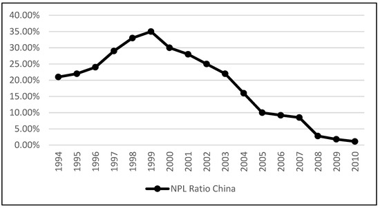
Figure 1.
NPL ratio in China from 1994 to 2010. Source: Elaboration from the data of the central bank of China statistics report and CBRC.
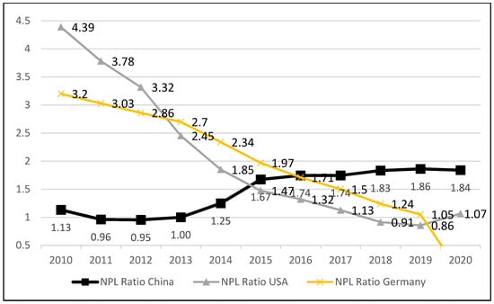
Figure 2.
NPL ratios of China, USA, and Germany from 2010–2020. Source: Elaboration of World Bank data.
It is evident from Figure 2 that the NPL ratio in China in recent years has trended in the opposite direction to that of the USA and Germany (used as a proxy for Europe). The drastic decrease in NPL ratio up to 2012 has a double explanation. First, the government chose to form asset management corporations (AMC), then state-owned asset management companies to take over bad loans from state-owned commercial banks. Another reason is that adequate supervision has been established to oversee the development of the banking system.
Figure 3 compares the China EPU with that of the USA and EU. According to the chart above, the uncertainty indices in China, Europe, and the USA are highly correlated, while the China index has a higher mean and volatility. Therefore, we must investigate the effects of the EPU on bad loans in China in order to estimate the efficiency of the institutional instruments of the various economic policies introduced by the government.
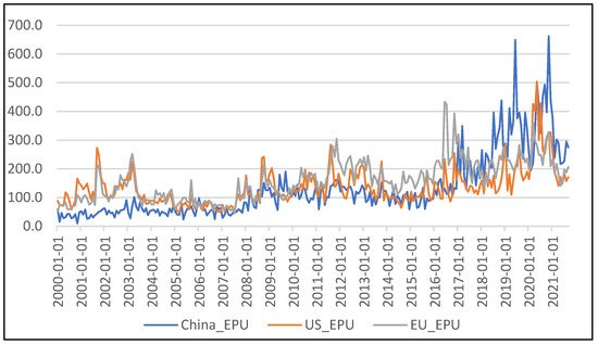
Figure 3.
Comparison of EPU indices in China, USA, and the European Union. Source: Elaboration of economic policy uncertainty data.
According to the literature, inflation (Klein 2013; Mazreku et al. 2018; Umar and Sun 2018) shows a significant negative relationship with NPLs. Furthermore, Figure 4 shows the trend of Consumer Price Index during several global crises, consequently affecting NPLs.. Further, Figure 5 depicts how the GDP growth rate suffered an important setback in the first quarter of 2020 due to the pandemic.
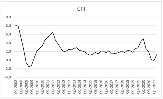
Figure 4.
Consumer Price Index growth rate based on seasonally adjusted volume data, percentage changes from the previous quarter.
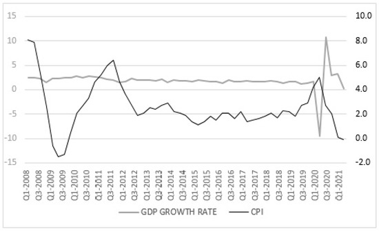
Figure 5.
Comparison of the trend of GDP growth rate and Consumer Price Index.
3.2. Methodology
The methodology used in this study was wavelet analysis. The wavelet approach is based on a coherent mathematical theory. Aguiar-Conraria et al. (2008) claim that it provides the possibility of uncovering transient relationships, in contrast to Fourier analysis. Furthermore, compared to the sine function, which is a large wave, wavelets are a small wave with finite support, so they are useful for locally approximating variables in space and time. The starting point of the analysis is what is known as mother wavelet ψ. Then, a variety of wavelets can be generated by scaling and translation.
where is a normalisation constant that guarantees that the wavelet has unit variance and and are the location and scale parameters that determine the exact position of the wavelet and wavelet dilation or stretch, respectively.
The discrete-time transform (DWR) and continuous form (CWT) are two versions of the wavelet transform. The continuous wavelet transform is an important instrument in economics, finance, and other fields. It is two-dimensional but depends on a one-dimensional signal, and it contains redundancy. There is little difference in continuous wavelet transform between adjacent scales when moving into larger scales, and there are slow variations across time at any fixed large scale.
The continuous wavelet transform, , is obtained by projecting onto the family
where * illustrates the complex conjugate. The continuous wavelet transform may also be represented in the frequency domain as
where indicates the Fourier transform of , determined as
and is the angular frequency.
A wavelet attempt is used in the paper, and the wavelet approach is included in the Morlet wavelet lineage. In addition, the Morlet wavelet is complex valued, which allows for the analysis of phase differences, i.e., lead–lag structures.
The wavelet power spectrum (WPS) is employed in this paper and is defined as:
The cross wavelet (continuous wavelet transform) reduces the time series factors. It is defined as
where * denotes the complex conjugate.
The cross-wavelet power spectrum is defined as
Wavelet coherency between two time series and can be interpreted as local correlation. The equation of squared wavelet coherence is defined as
where is a smoothing operator concerning time and scale, and represents a number between 0 and 1. When is closer to 1, it indicates that the time-series factors are connected at a particular dimension. This dimension is encircled by a black bar and is displayed in red. Furthermore, if the rate is closer to 0, there are no patterns between the series, and the blue line illustrates this graphically. For completeness, the analysis used wavelet coherence phase differences that depict details of the delays in oscillation (cycles) between the two time series of the variables under observation. Following the paper of Torrence and Webster (1999) we define the phase difference of the wavelet coherence as:
where symbolises an imaginary operator and represents the actual part of the operator in the previous equation. In the wavelet coherence diagram, the warmer coloured regions show the significant relationships between the variables, whereas the cold or blue area indicates low power between them. The arrows indicate whether the factors are in phase or anti-phase on the wavelet coherence plots.
The arrows surrounded by a thick black border indicate the amplitude of the importance of causality. The arrows pointing to the left reveal a negative link between the factors, while the arrows pointing to the right indicate positive connections. Furthermore, arrows pointing up, right up, or left down show that the second variable determines the first variable, while arrows pointing down, right down, or left up reveal that shifts in the first factor contribute considerably to changes in the second factor (Addison 2017).
The study explores the time–frequency relationship between NPLs and three different macro variables in China by applying the wavelet approach developed by Goupillaud et al. (1984). The investigation analyses the short-term and long-term relationship between the factors. Furthermore, a multiscale decomposition method produces an intrinsic pattern to indicate a frequency-related attitude to investigate the affiliation between NPL and macro variables in China. However, the wavelet coherency is limited to two variables and cannot be applied when multiple (≥3) variables are involved. It should be noted that the study purpose’s is to analyse and understand the relationships between pairs of variables for the correct interpretation of the direction and power that each has over the other.
4. Results
Figure 6 shows the progress of the NPL ratio and GDP growth rate in China since 2008 Q1. Economic growth was positive and almost constant over time, except for the years related to the first period of the COVID-19 outbreak.
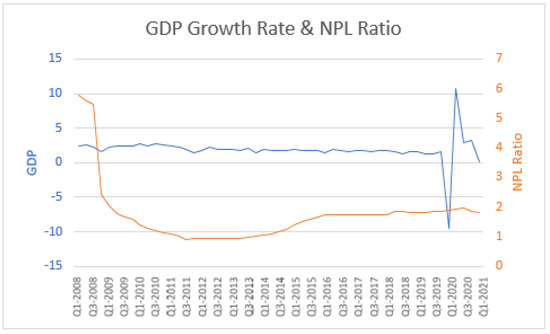
Figure 6.
Comparison between the NPL ratio and GDP growth rate.
There was a high NPL ratio until 2007 when the competent Chinese commission issued guidelines to strengthen the classification of bad loans and elucidate the criteria for estimating the volume necessary to cancel bad debts. From this point, non-performing loans decreased until 2014 and then increased once more.
The percentage of NPLs in China reflects the health of the banking system. However, a higher rate of such loans suggests that banks have difficulties collecting interest and principal from their customers. This could lead to lower profits for banks in China and possibly bank closures. Exploring the relationships between NPLs and GDP, NPLs and CPI, and NPLs and EPU is crucial for all countries and jurisdictions. However, a wavelet coherence approach capable of capturing both short- and long-term relationships has not been applied in any study on the co-movement of NPLs and macro variables in China. The methodology couples causality approaches based on the time and frequency domains. One of the wavelet method’s main benefits is to perform analyses that capture a larger image’s localised sub-image area.
Furthermore, the application of wavelet analysis allows evaluation of the degree of co-movements at different frequencies simultaneously. Thus, wavelet analysis differs from previously developed causality methods based on these features. In the present study, we fill this gap using an approach based on wavelet time- and frequency-based models.
In other terms, the paper aims to identify any relationship between NPLs and GDP, NPLs and CPI, and NPLs and EPU in China and whether these relationships are short or long term co-movement. Correspondingly, the wavelet power spectrum for NPLs, GDP, CPI and EPU is reported in Figure 7, Figure 8, Figure 9 and Figure 10. In addition, EPU and NPLs were transformed into quarterly growth to make the data homogeneous.
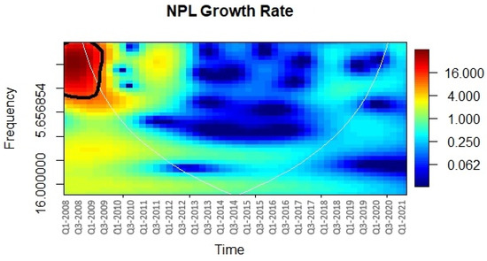
Figure 7.
WPS for NPL ratio growth rate. Note: The vertical axis presents frequencies (period), and the horizontal axis shows time.
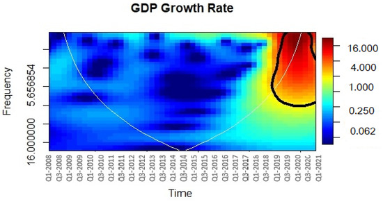
Figure 8.
WPS for GDP growth rate. Note: The vertical axis presents frequencies (period), and the horizontal axis shows time.
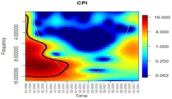
Figure 9.
Wavelet power spectrum for Consumer Price Index. Note: The vertical axis presents frequencies (period), and the horizontal axis shows time.
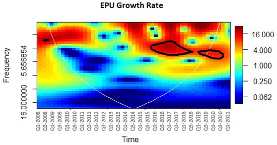
Figure 10.
Wavelet power spectrum for EPU index. Note: The vertical axis presents frequencies (period), and the horizontal axis shows time.
The regions with warmer colours (red) represent regions with significant inter-relation in the plot, while colder colours (blue) signify low power between the series. Cold regions beyond the lower significant areas represent any dependence between time and frequencies in the series. The arrows of the wavelet coherence plots indicate if the examined series are in lead/lag phase relations. When the two time series have zero phase difference, they move together at a particular scale. Arrows point to the right when the time series are in phase and point to the left when the time series are in anti-phase. When the two variables are in phase, they move in the same direction, while when they are in anti-phase, they move in opposite directions. Moreover, the direction of the arrows indicates what the variable that is leading is: when the arrows are pointing to the right-down or left-up, then the first variable is leading, and when the arrows are pointing to the right-up or left-down, then the second variable is leading (Addison 2017). The time horizon of the analysis is shown on the abscissa axis; the ordinate axis shows the frequency (the lower the frequency, the higher the scale). Wavelet coherence locates the regions where two time series covariate in time–frequency space.
Figure 7 indicates a high and statistically significant wavelet power spectrum for NPLs until 2009. Subsequently, the volatility has been lower. The blue part of the plot indicates low power, and red denotes high power. The area within the black line represents a significant effect at 5 per cent.
The wavelet power spectrum of the GDP growth rate (Figure 8) does not vary considerably over time. The period of the highest volatility was Q4 2019 to 2020. The highest point of the spectrum is at periodicities around the 0–3 quarter period. Due to zero padding or reflection, the data from the areas outside the white lines (“cone of influence”) are unreliable and are excluded from this analysis.
The CPI shows high volatility from 2008 to 2013, but only the period from 2011 to 2013 indicates statistically significant wavelet power. Subsequently, the volatility is lower (Figure 9).
The EPU growth rate has a high power at the scale of 3–6 quarter periods, indicating that there was uncertainty in China during the period 2015–2020 (Figure 10).
The wavelet analysis observed the co-movements between NPLs and three macroeconomic variables. Figure 11 shows wavelet coherence and reveals the strength of the correlation between NPLs and GDP in China. The results show that the coherence between NPLs and real GDP changes over time. In 2009–2010, there was a relevant correlation within the frequency of quarters three and four. Between 2011 and 2012 and in all quarters of 2015, the coherence broke down. For the most recent years, there was coherence for the eighth quarter. Therefore, GDP might not be a good determinant of the number of NPLs. In the plot, the cold areas outside the cone of influence represent time and frequencies without dependence on the variables.
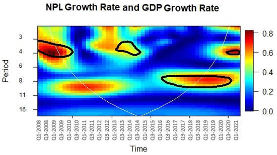
Figure 11.
Wavelet power coherence between NPLs and GDP. Note: The vertical axis presents frequencies (period), and the horizontal axis shows time.
In terms of the correlation value between NPLs and CPI regarding , the bright red colour indicates the higher correlation value. When analysing this figure, we concentrated on the arrows inside the significant area, which was accepted as the cone of influence. The direction of the arrows indicates the direction of the causality or correlation between NPLs and GDP.
Figure 12 shows that the arrows point left-down for Q1 2011 to Q3 2012. This means that the time series are anti-phase that move in the opposite direction. While, for the period from Q1 2014 to Q1 2015, the arrows pointing up and right mean that the time series move in the same direction (phase), with the first series leading the second one. Thus, it is evident that the dependence varies with time, which may be due to the period of rising CPI.
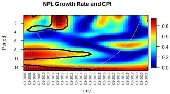
Figure 12.
Wavelet power coherence between NPLs and CPI. Note: The vertical axis presents frequencies (period), and the horizontal axis shows the time.
Figure 13 shows the different dynamics that connect the NPLs and EPU in the analysed time frame. It illustrates that the arrows point down and left at the end of the plot at the scale of 7 and 12 quarters (low frequency) in periods Q3 2010–Q3 2012, implying that in the medium-term, the EPU is essential for predicting NPLs in China. On the other hand, between Q1 2014 and Q 2016, the arrows point down, but at the top of the figure at the scale of 0–3 (high frequency), that is, in the short term, NPLs were leading EPU index.
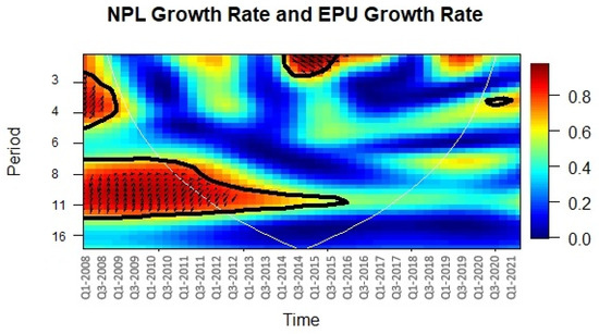
Figure 13.
Wavelet power coherence between NPLs and EPU. Note: The vertical axis presents frequencies (period), and the horizontal axis shows time.
For completeness, we carried out a robustness analysis through a linear Granger causality test that we report in the appendix (Appendix A).
5. Conclusions
In 2007, the Chinese authority responsible for the banking sector (CBIRC) issued guidelines by categorising NPLs and defining the criteria for the definition of reserves for bad loans. Further, in April 2019, they published a draft relating to the measures to be followed to manage NPL “Commercial Bank Financial Asset Risk Categorisation Provisional Measures”. Regulators sought to strengthen the risk-based classification requirement to speed up the recognition of bad loans. However, this measure was sidelined due to the pandemic. Moreover, the commission allowed banks to increase tolerance for NPLs taken out by small businesses affected by the pandemic. At present, China is entering a new economic phase; however, growth has slowed down, and a series of structural weaknesses are manifesting, while inflation is growing, fuelled by rising prices of raw materials and energy. In addition, there is concern regarding the liquidity and debt of important sectors like real estate, which is experiencing a profound crisis with some large operators in the industry at risk of bankruptcy.
The Chinese authorities have set rules and constraints on operators in this sector to bring their debt situation back to a sustainable level. However, this has highlighted their fragility and the risk of a domino effect in the financial sector.
In light of this situation, the relationship between non-performing loans and macroeconomic variables in China was analysed. Using quarterly data from 2008/Q1 to 2021/Q1 and through wavelet coherence analysis, the study evaluated causal relationships and short- and long-term connections. The main benefit of the wavelet analysis is to allow the time variation of movement of time series at various frequencies to be analysed efficiently and effectively. Furthermore, this methodology can be used to identify structural disruptions in terms of complete breakdowns of correlation or a shift in relevant frequency bands. The unique feature of the paper is its applied methodology, and particularly in its analysis of macro variables such as the EPU and CPI, which have never been considered in previous studies. Further, to our knowledge, there are no others works that have analysed the case of China.
The results show the relationship between NPLs and GDP growth rate. The figure of the wavelet coherence shows a zero-phase difference, which means that the two series move together on a medium period, with a high correlation but without indicating which variable is leading. This information leads to the assumption that GDP may not be the most appropriate determinant of NPLs in China. Regarding the connection between NPLs and CPI, the dependence is highly dynamic as it varies with time. Over a short time, the time series are anti-phase, while over a long time, the time series are in phase, with the NPLs series leading the CPI. The interesting finding may be due to an increase of the CPI. Another unique element is the consideration of the EPU index as a variable that influences NPLs in wavelet analysis. The EPU index has a notable influence on the number of NPLs. The results show that, in the short term, NPLs and EPU move in the same direction; thus, an increase of NPLs immediately increases EPU. In the long term, the time series are in anti-phase, which means they move in the opposite direction; the index (second variable) leads. By theorising that EPU will, in the long term, reduce NPLs, we can theorise that this will impact the size of bank loans by decreasing enterprises’ demand for and commercial banks’ supply of new credit funding. Whenever the EPU index increases, banks are able to lower loan sizes in order to improve their performance. EPU can also be modulated by marketisation levels and financial development depth that can affect enterprises and governments’ operational behaviour. Policymakers should take these intricate relationships into account. However, there are some limitations to the study. One limitation could be that it focuses only on China. The NPL ratio has steadily declined to reach the rate of 0.95% in 2012, increasing marginally over 2013−2020. They had and have a particular trend compared to NPL ratio of other countries, therefore this could have repercussions on the application of the results to other states. Moreover, some variables that may influence NPLs, such as unemployment rate, were not able to be considered.
Nevertheless, our study fills this research gap through an examination of how the short- and long-term movement of GDP, CPI, and the EPU influence China’s NPLs.
Further, the paper shows that in China, unlike other emergent economies (Kartal et al. 2021), GDP, one of the principal macro variables, does not impact the rate of NPLs. This result could be of note for the scientific literature as it prevents the comparison of the behaviour of other economies of emerging countries to China. It would be interesting, in further studies, to make a comparison with the major world economies, such as the USA and EU, through the same methodology and expand the variables used (interest rate, employment/unemployment rate). In addition, it would be interesting to investigate the relationships with microeconomic variables to permit governments, investors, and managers to have a complete tool that supports decision-making.
Author Contributions
Conceptualisation, E.D.F.; methodology, E.D.F.; software, E.D.F.; validation, E.D.F.; formal analysis, E.D.F.; investigation, E.D.F.; resources, E.D.F.; data curation, E.D.F.; writing—original draft preparation, E.D.F.; writing—review and editing, E.D.F.; visualisation, E.D.F.; supervision, E.A. All authors have read and agreed to the published version of the manuscript.
Funding
This research received no external funding.
Informed Consent Statement
Informed consent was obtained from all subjects involved in the study.
Data Availability Statement
Research data are available from authors upon request.
Acknowledgments
I thank two anonymous referees for their helpful suggestions and comments.
Conflicts of Interest
The authors declare no conflict of interest.
Appendix A. Robustness Check: Linear Granger Causality Test
For two stationary series, and , the linear causality test is based on vector autoregressive model (VAR) representation of the two series, as follows:
where is the lag length and variables. In this case, the criterion selected to determine the lag length was the Schwarz information criterion. Through testing, we determined two through the test, we determine two null hypothesis: (I) do not cause which is indicated as ; and (II), do not cause which is indicated as . In the first hypotheses, causality runs from to when the null is rejected; in the second hypotheses, causality runs from to when the null is rejected; and, finally, bivariate causality means that both hypotheses are rejected.

Table A1.
Linear Granger causality test.
Table A1.
Linear Granger causality test.
| Time Scale | Lags | Result | Null Hypothesis | |||
|---|---|---|---|---|---|---|
| GDP does not Granger Cause NPL | NPL does not Granger Cause GDP | |||||
| GDP&NPL | 2 | No causality | F-test | p-Value | F-test | p-Value |
| 0.66413 | 0.5196 | 0.62 | 0.5424 | |||
| CPI does not Granger Cause NPL | NPL does not Granger Cause CPI | |||||
| CPI&NPL | 2 | Causality | F-test | p-Value | F-test | p-Value |
| 2.67245 | 0.0798 | 1.33689 | 0.2727 | |||
| EPU does not Granger Cause NPL | NPL does not Granger Cause EPU | |||||
| EPU&NPL | 3 | Causality | F-test | p-Value | F-test | p-Value |
| 7.185 | 0.0005 | 0.38485 | 0.7644 | |||
Notes: Lags in tests were chosen using Schwarz Information Criterion.
The linear Granger causality (Granger 1969) results validate the results obtained through the wavelet analysis, remembering that in any case, the wavelet is a “dynamic” methodology while the robustness test is static.
References
- Addison, Paul S. 2017. The Illustrated Wavelet Transform Handbook: Introductory Theory and Applications in Science, Engineering, Medicine and Finance. Boca Raton: CRC Press. [Google Scholar]
- Aguiar-Conraria, Luís, Nuno Azevedo, and Maria Joana Soares. 2008. Using wavelets to decompose the time–frequency effects of monetary policy. Physica A: Statistical Mechanics and Its Applications 387: 2863–78. [Google Scholar] [CrossRef]
- Ahmed, Shakeel, M. Ejaz Majeed, Eleftherios Thalassinos, and Yannis Thalassinos. 2021. The Impact of Bank Specific and Macro-Economic Factors on Non-Performing Loans in the Banking Sector: Evidence from an Emerging Economy. Journal of Risk and Financial Management 14: 217. [Google Scholar] [CrossRef]
- Arestis, Philips, and Maggie Mo Jia. 2019. Credit risk and macroeconomic stress tests in China. Journal of Banking Regulation 20: 211–25. [Google Scholar] [CrossRef]
- Arham, Nurfilzah, Mohd Shamlie Salisi, Rozita Uji Mohammed, and Jasman Tuyon. 2020. Impact of macroeconomic cyclical indicators and country governance on bank non-performing loans in Emerging Asia. In Eurasian Economic Review. Berlin and Heidelberg: Springer, vol. 10, pp. 707–26. [Google Scholar]
- Baker, Scott R., Nicholas Bloom, and Steven J. Davis. 2013. Measuring Economic Policy Uncertainty, Chicago Booth Paper. Stanford: Department of Economics, Stanford University, vol. 83. [Google Scholar]
- Balgova, Maria, Michel Nies, and Alexander Plekhanov. 2018. The Economic Impact of Reducing Non-Performing Loans. SSRN Electronic Journal. [Google Scholar] [CrossRef]
- Berti, Katia, Christian Engelen, and Bořek Vašíček. 2017. Quarterly Report on the Euro Area, Quarterly Report on the Euro Area. Luxembourg: Publications Office of the Europe Union, vol. 16. [Google Scholar] [CrossRef]
- Borio, Claudio, Mathias Drehmann, and Kostas Tsatsaronis. 2012. BIS Working Papers Stress-Testing Macro Stress Testing: Does It Live Up to Expectations? Available online: www.bis.org (accessed on 10 December 2021).
- Chi, Qinwei, and Wenjing Li. 2017. Economic policy uncertainty, credit risks and banks’ lending decisions: Evidence from Chinese commercial banks. China Journal of Accounting Research 10: 33–50. [Google Scholar] [CrossRef]
- Cucinelli, Doriana. 2015. The Impact of Non-performing Loans on Bank Lending Behavior: Evidence from the Italian Banking Sector. Eurasian Journal of Business and Economics 8: 59–71. [Google Scholar] [CrossRef]
- Davis, Steven J., Dingqian Liu, and Xuguang S. Sheng. 2019. Economic Policy Uncertainty in China Since 1949: The View from Mainland Newspapers. Working Paper. pp. 1–35. Available online: https://static1.squarespace.com/static/5e2ea3a8097ed30c779bd707/t/5f7f49d054a84229354fe9ab/1602177496854/EPU+in+China%2C+View+from+Mainland+Newspapers%2C+August+2019.pdf (accessed on 1 December 2021).
- European Central Bank. 2017. Guidance to Banks on Non-Performing Loans. Banking Supervision, No. March. Frankfurt: European Central Bank, pp. 1–131. [Google Scholar]
- Farhan, Muhammad, Ammara Sattar, Abrar Hussain Chaudhry, and Fareeha Khalil. 2012. Economic determinants of non-performing loans: Perception of Pakistani bankers. European Journal of Business and Management 4: 87–99. [Google Scholar]
- Feng, Yi. 2001. Political freedom, political instability, and policy uncertainty: A study of political institutions and private investment in developing countries. International Studies Quarterly 45: 271–94. [Google Scholar] [CrossRef]
- Goupillaud, Pierre, Alex Grossmann, and Jean Morlet. 1984. Cycle-octave and related transforms in seismic signal analysis. In Geoexploration. Amsterdam: Elsevier, vol. 23, pp. 85–102. [Google Scholar]
- Granger, Clive J. W. 1969. Investigating causal relations by econometric models and cross-spectral methods. Econometrica: Journal of the Econometric Society 37: 424–38. [Google Scholar] [CrossRef]
- IMF. 2005. The Treatment of Nonperforming Loans. Paper presented at Eighteenth Meeting of the IMF Committee on Balance of Payments Statistics, Washington, DC, USA, June 27–July 1; pp. 1–15. [Google Scholar]
- Kartal, Mustafa Tevfik, Derviş Kirikkaleli, and Fatih Ayhan. 2021. Nexus between non-performing loans and economic growth in emerging countries: Evidence from Turkey with wavelet coherence approach. International Journal of Finance and Economics. [Google Scholar] [CrossRef]
- Klein, Nir. 2013. Non-Performing Loans in CESEE: Determinants and Impact on Macroeconomic Performance. IMF Working Papers. Washington, DC: International Monetary Fund, vol. 13, p. 1. [Google Scholar]
- Le, Quan, and Paul J. Zak. 2001. Political Risk and Capital Flight, Claremont Colleges Working Papers in Economics. Available online: http://hdl.handle.net/10419/94628www.econstor.eù (accessed on 13 December 2021).
- Lu, Yunxuan. 2020. Study of Non-Performing Loans in China, Massachusetts Institute of Technology Sloan School of Management. Available online: https://dspace.mit.edu/handle/1721.1/127068%0Ahttps://dspace.mit.edu/bitstream/handle/1721.1/127068/1191819124-MIT.pdf?sequence=1&isAllowed=y (accessed on 1 December 2021).
- Mazreku, Ibish, Fisnik Morina, Valdrin Misiri, Jonathan V. Spiteri, and Simon Grima. 2018. Determinants of the Level of Non-Performing Loans in Commercial Banks of Transition Countries. European Research Studies Journal 21: 3–13. [Google Scholar] [CrossRef]
- Mo, Yk. 1999. A review of recent banking reforms in China. BIS Policy Papers 7: 90–109. [Google Scholar]
- Nouaili, Makram, Ezzeddine Abaoub, and Anis Ochi. 2015. The determinants of banking performance in front of financial changes: Case of trade banks in Tunisia. International Journal of Economics and Financial Issues 5: 410–17. [Google Scholar]
- Rajha, Khaled Subhi. 2016. Determinants of Non-Performing Loans: Evidence from the Jordanian Banking Sector. Journal of Finance and Bank Management 4: 125–36. [Google Scholar] [CrossRef][Green Version]
- Torrence, Christopber, and Peter J. Webster. 1999. Interdecadal Changes in the ENSO–Monsoon System. Journal of Climate 12: 2679–2690. [Google Scholar] [CrossRef]
- Umar, Muhammad, and Gang Sun. 2018. Determinants of non-performing loans in Chinese banks. Journal of Asia Business Studies 12: 273–89. [Google Scholar] [CrossRef]
- Wood, Anthony, and Nakita Skinner. 2018. Determinants of non-performing loans: Evidence from commercial banks in Barbados. The Business and Management Review 9: 44–64. [Google Scholar]
- Zeng, Shihong. 2012. Bank Non-Performing Loans (NPLS): A Dynamic Model and Analysis in China. Modern Economy 3: 100–10. [Google Scholar] [CrossRef]
Publisher’s Note: MDPI stays neutral with regard to jurisdictional claims in published maps and institutional affiliations. |
© 2022 by the authors. Licensee MDPI, Basel, Switzerland. This article is an open access article distributed under the terms and conditions of the Creative Commons Attribution (CC BY) license (https://creativecommons.org/licenses/by/4.0/).