Classifying Insurance Reserve Period via Claim Frequency Domain Using Hawkes Process

Abstract

In this paper, the insurance reserve period will be classified according to the claim frequency domain, such as high- or low-frequency periods. We use the clustering method to create and group claims data according to their frequency period. Meanwhile, we use a risk process to mimic and predict the movement of the reserve from time to time in each group of claim period that is formed. The risk process model used here is the Hawkes process, which is a one-dimensional simple point process and a special type of self-exciting process. Based on this process, we will estimate the reserve at a certain date in the future and the average historical reserve for each group period.

1. Introduction

In non-life insurance, a huge amount of personal experience exists with some extremely big hazards. A multi-billion-dollar manufacturing company might, for instance, take out workers’ compensation, commercial liability, and property damage insurance for its several plants. An insurer may be able to determine the appropriate reserve for these risks using the risk’s unique experience.

However, it is not prudent to establish reserves only using the historical behavior of the risk for the entire claim period and ignoring the pattern of claims frequency that may occur within the claim periods. In these situations, it is necessary to analyze risks using classification of risk process according to the claim frequency domain, which involves grouping risks with comparable loss potential and imposing new various manual rates to accommodate for variations in loss potential within the groupings.

Moreover, we can use risk theory to model random processes that will explain the occurrence of claims. The traditional Cramer-Lundberg risk model, developed by Lundberg (1903), has undergone several studies in recent years. Lefevre and Picard (2006) for instance, developed a risk model in which the successive claim amounts are independent and non-identically distributed while Romaniuk (2019) described the application of fuzzy sets to the risk process, especially fuzzy numbers to model the possible penalties which are related to the ruin event. Many studies, including Raducan et al. (2015), describe a risk process with claim costs modeled by Erlang or a mixture of exponential distributions and examine the calculation of ruin probability with independent and non-homogeneously distributed claim costs.

The application of self-exciting Hawkes processes in risk theory, which was first introduced by Hawkes (1971), is also covered in several works. Due of their capacity to reflect endogenously generated clustering, these processes have attracted attention. This method is used by Swishchuk et al. (2021) because it enables the use of practical diffusion approximation results from the risk model with claims arrivals based on a general compound Hawkes process using real empirical data, allowing for the realistic representation of claim costs.

Furthermore, Jeong and Zou (2022) proposed a dynamic credibility model for claim count that extends the benchmark Poisson generalized linear models (GLM) by incorporating self-excitation and exponential decay features from Hawkes processes. Bessy-Roland et al. (2021) proposed a multivariate Hawkes framework for modeling and predicting cyber-attacks frequency. They demonstrated the ability of Hawkes models to capture self-excitation and interactions of data-breaches depending on their type and targets.

In this paper, we provide a novel approach for concurrently categorizing and estimating insurance reserves using the Hawkes process. In this approach, we first categorize the data in accordance with the frequency of claims and then use the Hawkes process risk model for each newly formed group to estimate its reserve. This method has the advantage of allowing us to classify claim data by the risk category involved while also estimating reserves. In addition, there are two phenomena that are common to reserves over time. First, past claims tend to increase reserves, and second, recent claims have a greater impact on reserves than outdated claims. These phenomena are very suitable to be modeled with the Hawkes process which has two main features, namely self-excitation and exponential decay.

This paper is organized as follows: Section 2: Preliminary research and Methodologies, which consists of a discussion of the cluster analysis used in this study to classify the claim period and the Hawkes process that we use in modeling the movement of reserves. Then, in Section 3: Results and Discussions, we describe the data we used in this study. Then we perform a clustering procedure to obtain groups of different claim periods based on their frequency. After that, we continue with the reserve process modeling using the Hawkes process for each claim period formed from the previous steps. At the end of this section, we discuss some of the important findings of our methodology and further study opportunities to develop better models. The last, Section 4, is devoted to the conclusion.

2. Preliminary Research and Methodologies

Two significant methodologies that underpin our study are described in this section: pairing the Hawkes process with cluster analysis.

2.1. Cluster Analysis

Cluster analysis is a part of multivariate analysis that aims to partition objects into several clusters. Each cluster is homogeneous concerning the specific characteristics, i.e., observations in each group are similar to each other. Each group should be different from other groups concerning the same features; that is, the objects of one group should be different from the things of other groups. The principle of clustering objects is to obtain a measure of proximity that explains the similarity between objects. This proximity between objects is calculated based on the type of data.

2.1.1. Hierarchical Method

The hierarchical clustering method moves forward either through a series of subsequent divisions or mergers. The individual items are the first step in the agglomerative hierarchical technique. In the beginning, there are therefore as many clusters as objects. First, groups of the objects that share the most similarities are formed, and then these initial groups are combined based on their commonalities. All the subgroups eventually combine into a single cluster when the similarity lowers. See for example Kaufman and Rousseeuw (1990).

As in Johnson and Wichern (2009), the agglomerative hierarchical clustering for N objects is such as below:

(i)

Start with N clusters, each containing a single entity and an $N\times N$ symmetric distances (or similarities) $D=\left\{d_{ik}\right\};i=k=1,2,3,\dots ,n$. In this paper, we use the Euclidean distance. Suppose object i and object j on data sets, then the Euclidean distance is formulated as follows:

$$d(i,j)=\sqrt{\sum _{l=1}^p{(x_l^i-x_l^j)}^2}.$$

(1)

where p is the number of variables.

(ii)

Search the nearest (most similar) pair of objects (e.g., object or cluster U and object or cluster V) from the distance matrix.

(iii)

Merge clusters U and V, label them $\left(UV\right)$ and then update the distance matrix entries by

(a)

deleting the rows and columns corresponding to clusters U and V and

(b)

adding a row and column indicating the distance between the merged cluster (UV) and the remaining clusters.

(iv)

Repeat steps (ii) and (iii) an additional $N-1$ times. (All objects will be in a single cluster after the algorithm terminates).

This paper uses complete linkage to merge clusters U and V in Step 3. Suppose two cluster U and cluster V have the nearest distance $d_{UV}$, with $d_{UW}$ is the distance between cluster U and cluster W, while $d_{VW}$ is the distance between cluster V and cluster W. The distance between cluster $\left(UV\right)$ and any cluster W is computed by

$$d_{\left(UV\right)W}=max(d_{UW};d_{VW}).$$

(2)

2.1.2. Estimation of the Number of Clusters

One of the problems that often draws attention in cluster analysis is determining the optimal group number. Several methods for estimating the number of clusters were developed using a measure of homogeneity within a group $W_k$. See for instance Johnson and Wichern (2009), which was formulated as follows:

$$\underset{p\times p}{W_k}=\sum _{g=1}^k\sum _{i=1}^{n_g}(\underset{p\times 1}{x_{g_i}}-\underset{p\times 1}{{\overline{x}}_g})(\underset{p\times 1}{x_{g_i}}-\underset{p\times 1}{{\overline{x}}_g}){}^t.$$

(3)

where p is the number of variables, $n_g$ is the number of group g, $(g=1,2,\dots ,k)$, $x_{g_i}$ is the ith object $(i=1,2,\dots ,k)$ on the group g and ${\overline{x}}_g$ is the average of variable in the group g.

Hartigan (1975) proposes the index to determine the number of clusters based on a trace of homogeneity within groups. Hartigan’s index is defined as follows:

$$H\left(k\right)=\left(\frac{\mathrm{tr}\left(W_k\right)}{\mathrm{tr}\left(W_{k+1}\right)}\right)(n-k-1)$$

(4)

where $\mathrm{tr}\left(W_k\right)$ is the trace of a square matrix $W_k$. The number of clusters is the smallest of $k(k\ge 1)$, so Hartigan’s index is less than ten $\left(H\right(k\left)\right)\le 10$.

2.2. Hawkes Process

2.2.1. Hawkes Process for Claim Arrivals Distribution

Hawkes process is a one-dimensional simple point process and a special type of self-exciting process. It was introduced by Hawkes (1971). Consider $N\left(t\right),t\ge 0$, a counting process with history $\mathcal{H}\left(t\right),t\ge 0$ that satisfy:

$$\begin{array}{c}\hfill \mathbb{P}\left(N\right(t+h)-N(t)=m|\mathcal{H}\left(t\right))=\\ \hfill \left\{\begin{array}{cc}{\lambda }^{\ast }\left(t\right)h+o\left(h\right),\hfill & m=1\hfill \\ o\left(h\right),\hfill & m>1\hfill \\ 1-{\lambda }^{\ast }\left(t\right)h+o\left(h\right),\hfill & m=0.\hfill \end{array}\right.\end{array}$$

(5)

A simple and conditional orderly self-exciting point process N on $[0,\infty )$ is called Hawkes process if the conditional intensity function is in the form:

$${\lambda }^{\ast }\left(t\right)=\lambda +{\int }_0^t\mu (t-s)dN\left(s\right).$$

(6)

where $\lambda >0$ is the background rate of the process N and where $\mu (·)$ is a function which governs the clustering density of N. The function $\mu (·)$ is sometimes called the exciting function or the excitation function of N and to avoid treating the homogeneous Poisson process as a trivial case, we assume that $\mu (·)\ne 0$.

In addition, the function (6) also can be written as:

$${\lambda }^{\ast }\left(t\right)=\lambda +\sum _{t_i<t}\mu (t-t_i)$$

(7)

with the observed sequence of past arrival $\{t_1,t_2,...,t_k\}$, basic conditional intensity $\lambda >0$ and excitation function $\mu (·)$.

One of the common choices for excitation function is the exponential decay function. In this case, $\mu \left(t\right)=\alpha e^{-\beta t}$ with $\alpha ,\beta >0$, so that the exponentially decaying intensity function becomes

$${\lambda }^{\ast }\left(t\right)=\lambda +{\int }_0^t\alpha e^{-\beta (t-s)}dN\left(s\right)=\lambda +\sum _{t_i<t}\alpha e^{-\beta (t-t_i)}.$$

(8)

In this case, $\alpha$ and $\beta$ can be interpreted as each arrival in the system instantaneously increases the arrival intensity by $\alpha$, then over time this arrival’s influence decays at rate $\beta$.

To model a process from some time before the beginning of the observation period or after it is started, initial condition ${\lambda }^{\star }\left(0\right)={\lambda }_0$ can be set. The stochastic differential equation

$$d{\lambda }^{\ast }\left(t\right)=\beta (\lambda -{\lambda }^{\ast }\left(t\right))d\left(t\right)+\alpha dN\left(t\right),t\ge 0$$

(9)

must be satisfied for this scenario. If the stochastic equation above applied, the general solution can be written as

$${\lambda }^{\ast }\left(t\right)=e^{-\beta t}({\lambda }_0-\lambda )+\lambda +{\int }_0^t\alpha e^{-\beta (t-s)}dN\left(s\right),t\ge 0,$$

(10)

which is an extension of (8).

We restrict ourselves to the Markovian Hawkes process in this study. Generally speaking, the Hawkes process can be non-Markovian. When the excitation function is represented by the sum of exponential functions (8), the Hawkes process is Markovian. See, for instance Gao and Zhu (2017).

2.2.2. Distributional Properties and Auto Correlation Function

Da Fonseca and Zaatour (2013) demonstrated that for a Hawkes process with the conditional intensity function follows (9), the expected value and variance of the number of jumps during a $\tau$-length interval when t goes to infinity are given by

$$\begin{array}{cc}\hfill \mathbb{E}\left[N\right(\tau \left)\right]& =\underset{t\to \infty }{lim}\mathbb{E}[N(t+\tau )-N\left(t\right)]=\frac{\lambda }{1-\frac{\alpha }{\beta }}\tau \hfill \end{array}$$

(11)

$$\begin{array}{cc}\hfill \mathrm{Var}\left[N\right(\tau \left)\right]& =\underset{t\to \infty }{lim}\mathbb{E}\left[{\{N(t+\tau )-N\left(t\right)\}}^2\right]-\mathbb{E}{\left[N\left(\tau \right)\right]}^2\hfill \\ \hfill & =\frac{\lambda \beta }{\beta -\alpha }\left[\tau {\left(\frac{\beta }{\beta -\alpha }\right)}^2+\left(1-{\left(\frac{\beta }{\beta -\alpha }\right)}^2\right)\frac{1-e^{-\tau (\beta -\alpha )}}{\beta -\alpha }\right].\hfill \end{array}$$

(12)

Then, as t goes to infinity, the following formula can be used to calculate the covariance of the arrival rate given two $\tau$-length intervals with lag $\delta >0$ that are not overlapping:

$$\begin{array}{cc}\hfill \mathrm{Cov}\left(N\right(\tau ),\delta )& =\underset{t\to \infty }{lim}(\mathbb{E}\left[(N(t+\tau )-N\left(t\right))(N(t+2\tau +\delta )-N(t+\tau +\delta ))\right]\hfill \\ & -\mathbb{E}\left[N\right(\tau \left)\right]\mathrm{E}(t+\tau +\delta ,\tau ))\hfill \\ \hfill & =\frac{\lambda \beta \alpha (2\beta -\alpha ){(e^{(\alpha -\beta )\tau }-1)}^2}{2{(\alpha -\beta )}^4}{e}^{(\alpha -\beta )\delta }.\hfill \end{array}$$

(13)

Keep in mind that this necessitates the process’s stability, which suggests $\alpha <\beta$. As a consequence of this result, we can obtain the auto correlation function of the process as the following:

$$\mathrm{Acf}(\tau ,\delta )=\frac{e^{-2\beta \tau }{(e^{\alpha \tau }-e^{\beta \tau })}^2\alpha (\alpha -2\beta )}{2(\alpha (\alpha -2\beta )(e^{(\alpha -\beta )\tau }-1)+{\beta }^2\tau (\alpha -\beta )}{e}^{(\alpha -\beta )\delta }.$$

(14)

2.2.3. Parameter Inference

The maximum likelihood estimation method is one way to fit empirical data to an exponentially decaying Hawkes process. With this approach, as in Laub et al. (2015), we first identify the (log-) likelihood function and estimate the model parameters as the inputs that maximize this function. The log-likelihood function of Hawkes process for the interval $[0,T]$ can be written as

$$\ell =\sum _{i=1}^{N\left(T\right)}\log (\lambda +\alpha A\left(i\right))-\lambda T+\frac{\alpha }{\beta }\sum _{i=1}^{N\left(T\right)}(e^{-\beta (T-t_i)}-1).$$

(15)

where

$$A\left(i\right)=\left\{\begin{array}{cc}0,\hfill & i=1\hfill \\ \sum _{j=1}^{i-1}{e}^{-\beta (t_i-t_j)}=e^{-\beta (t_i-t_{i-1})}(1+A(i-1)),\hfill & i\in \{2,\dots ,k\}].\hfill \end{array}\right.$$

(16)

It is clear that maximum likelihood estimation will usually be very effective for model fitting. However, Filimonov and Sornette (2015) found certain drawbacks to using this method, including problems with bias in small sample sizes but performance issues with large samples. Another numerical disadvantage that might occur with this method is the outcome can be constrained to local optimization. These problems served as the impetus for Da Fonseca and Zaatour (2013) to develop the method of moments for parameter estimation. Zaatour (2014) developed an R package |hawkes|implementing this routine in C++ in an attempt to mitigate the performance issues. The recent trend of performing parameter estimation using the generalized method of moments is primarily due to this “performance bottleneck”. Da Fonseca and Zaatour (2013) claim that the process is “immediate” in their test sets. The technique makes use of sample moments and the sample autocorrelation function, which are smoothed using a (ad hoc) user-selected process.

2.2.4. Goodness of Fit by Simulations

With regard to our situation, we will use Hawkes process simulation to assess the model’s fitness. Ogata (1981) shows a simulation method of point processes, one of which is the Hawkes’ self-exciting process, with the intensity function stated in (6) and the log-likelihood function stated in (15). For the simulations, Ogata (1981) used the likelihood function of the simulated data rewritten as:

$$L_t({\alpha }_0,\dots ,{\alpha }_p,\beta )=\sum _{i-1}^{n}log\{\mu +\sum _{j=0}^p{\alpha }_j{R}_j\left(i\right)\}-\mu T-\sum _{i=1}^n\sum _{j=0}^p{\alpha }_j{S}_j(T-t_i).$$

(17)

The function $R_j\left(i\right)$ and $S_j\left(i\right)$ are given recursively for $j=0,1,2,\dots$ and $i=2,3,\dots$, as:

$$R_j\left(i\right)=A_j(t_i-t_{i-1})+\sum _{k=0}^j{}_j{C}_k{A}_{j-k}(t_i-t_{i-1})R_k(i-1).$$

(18)

and

$$S_{j+1}\left(t\right)=\frac{\{(j+1)S_j\left(t\right)-A_{j+1}\left(t\right)\}}{\beta }.$$

(19)

where ${}_j{C}_k$ denotes a binomial coefficient and initial values are set as:

$$\lambda \left(t_{n+1}\right|t_1,\dots ,t_n)=\mu +\sum _{j=0}^p{\alpha }_j{R}_j(n+1).$$

(20)

2.3. Markov Chain for Claim Cost Distribution

In actuarial studies, the claim costs $\left\{Y_i\right\}$ are typically assumed to be independent and identically distributed with distribution D. We also assumed $m_1=\mathbb{E}\left[Y_1\right]$ and $m_2=\mathbb{E}\left[Y_1^2\right]$ are the first and the second finite moments of D, respectively. We follow Swishchuk et al. (2021) and apply the theoretical findings for general compound Hawkes processes, which they assumed independence between subsequent claim costs.

Hawkes process could be used to model arrival sequence to a system over time (Ogata (1999)). Hawkes process arrivals and independent and identically distributed claim costs were examined by Stabile and Torrisi (2010) and Cheng and Seol (2020) in relation to risk models. However, for those models, it is difficult to immediately apply the result to empirical data, and the only way to determine ruin probabilities is numerically. Then, based on the empirical distribution of observed claim costs, we approximate an independent and identically distributed sequence using the Markov chain ($Z_i$) and the function $a\left(z\right)$. By expanding the Markov chain’s N number of states, the approximation can be made to fit any set of data arbitrarily well.

If G is the largest claim cost that has been observed and $\widehat{D}$ is the empirical distribution function of claim costs, then $\widehat{D}\left(G\right)$ equals 1. We created equally spaced boundaries $(g_1,g_2,...,g_N=G)$ and specify $p^{\star }=(p_1^{\star },\dots ,p_N^{\star })$ as

$$\begin{array}{cc}\hfill p_1^{\star }& =\widehat{D}\left(g_1\right)\hfill \\ \hfill p_2^{\star }& =\widehat{D}\left(g_2\right)\hfill \\ \hfill \cdots \\ \hfill p_N^{\star }& =\widehat{D}\left(g_N\right)-\sum _{i=1}^{N-1}{p}_i^{\star }=1-\sum _{i=1}^{N-1}{p}_i^{\star }.\hfill \end{array}$$

(21)

Hence, by the definition ${\sum }_{i=1}^N{p}_i^{\star }=1$.

Consider that $Z_i$ is a Markov chain on finite state space $\{1,\dots ,N\}$ with

$$P=\left(\begin{array}{cccc}{p}_1^{\star }& p_2^{\star }& \cdots & p_N^{\star }\\ \cdots & \cdots & \cdots & \cdots \\ p_1^{\star }& p_2^{\star }& \cdots & p_N^{\star }\end{array}\right)=\left[\begin{array}{c}{p}^{\star }\\ ⋮\\ p^{\star }\end{array}\right]$$

(22)

as its transition matrix. Please note that because in a finite state space, the elements of P are the same for each row, then $\left(Z_i\right)$ is an irreducible Markov chain. This means the process can go from any state to any state, whatever the number of steps it requires.

Furthermore, for each state $k\in Z$ we can see that the columns of P remain constant, thus $\mathbb{P}(Z_{i+1}=k|Z_i=j)=\mathbb{P}(Z_{i+1}=k|Z_i=I)=p_k^{\star }$ where $\forall j,I\in N$. We can also have the following:

$$\begin{array}{c}\hfill \mathbb{P}(Z_{i+1}=k)=\sum _{j\in Z}\mathbb{P}(Z_{i+1}=k|Z_i=j)=p_k^{\star }\sum _{j\in Z}\mathbb{P}(Z_i=j)=p_k^{\star }\\ \hfill \forall k\in Z,i\in \mathbb{N}\end{array}$$

(23)

using the total probability rule and Markov property. The probability of realizing one state is also independent of the probability of realizing the preceding state, therefore $\left(Z_i\right)$ completely defines an independent and identically distributed sequence. We then let Y be a random variable with distribution function $\widehat{D},A_i:=\{\omega :Y\left(\omega \right)\in (g_i-1,g_i]\}$, and set

$$\begin{array}{cc}\hfill a\left(i\right)& =E\left[Y\right|g_{i-1}<Y\le g_i]=E\left[Y\right|A_i]\hfill \\ \hfill & =\frac{\mathbb{E}\left[Y{\mathbf{1}}_{A_i}\right]}{\mathbb{P}\left(A_i\right)}=\frac{\mathbb{E}\left[Y{\mathbf{1}}_{A_i}\right]}{p_i^{\star }}.\hfill \end{array}$$

(24)

Therefore, the expected value of the claim cost can be derived as follows:

$$a^{\star }=\sum _{i=1}^N{p}_i^{\star }a\left(i\right)=\sum _{i=1}^N\mathbb{E}\left[Y{\mathbf{1}}_{A_i}\right]=\mathbb{E}\left[Y\right].$$

(25)

In this case, $a\left(Z_i\right)$ depicts an independent and identically distributed sequence that close to approximating the distribution $\widehat{D}$ in terms of the number of states N goes to infinity.

2.4. Hawkes Process Implementation in Risk Modeling

A risk model typically takes the form of the following and aims to describe the capital that an insurance company, or a portion of it, will have available over time:

$$R=u+ct-\sum _{i=1}^{N_t}{Y}_i.$$

(26)

In the above formula, u is the underlying initial capital while c is the premium rate whose value does not change over time. $N\left(t\right)$ is a counting process that portraying the quantity of cases happening in the time interval $[0,t]$ while $\left\{Y_i\right\}$ is arrangement of non-negative random variables depicting the claim cost. Typically, the $\left\{Y_i\right\}$ are independent and identically distributed non-negative random variables with distribution F and $E\left[Y_1\right]=m_1$ and $E\left[Y_1^2\right]=m_2$. $N\left(t\right)$ and $\left\{Y_i\right\}$ are also thought to be independent. In the traditional situation, $N\left(t\right)$ is a homogeneous Poisson measure; however, going forward, we will consider that $N\left(t\right)$ is a fixed Hawkes measure with extremely decaying effect.

Definition 1

(Risk Model with General Compound Hawkes Process Swishchuk (2017)). Let $N\left(t\right)$ be any one-dimensional Hawkes process. Let $\left(Z_i\right)$ be an ergodic continuous-time finite (or countably infinite) Markov Chain, independent of $N\left(t\right)$, with state space Z, and let $a\left(z\right)$ be any bounded function

$$H\left(t\right)=H\left(0\right)+\sum _{i=1}^{N\left(t\right)}a\left(Z_i\right).$$

(27)

The risk process $R\left(t\right)$ based on a general compound Hawkes process can be defined as

$$R\left(t\right)=\sum _{k=1}^n{u}_k+ct-\sum _{k=1}^n\sum _{i=1}^{N\left(t\right)}{a}_k\left(Z_i\right).$$

(28)

where n is the number of groups by clustering.

In this definition, $\left(Z_i\right)$ is a continuous-time Markov chain on the state space $Z=\{1,\dots ,n\}$, while $N\left(t\right)$ is a Hawkes process. In addition, $a\left(z\right)$ is a bounded function on Z while we also assume $N\left(t\right)$ and $\left(Z_i\right)$ are independent.

Theorem 1

(Law of Large Numbers for General Compound Hawkes Processes Swishchuk (2017)). Let $R\left(t\right)$ be the risk model defined in Definition 1, and let $\left(Z_i\right)$ be a Markov Chain with state space Z and stationary probabilities $p_i^{\star }$.

Suppose that $0<\widehat{\mu }={\int }_0^{\infty }\mu \left(s\right)ds<1$. Then

$$\underset{t\to \infty }{lim}\frac{R\left(t\right)}{t}=c-a^{\star }\frac{\lambda }{1-\widehat{\mu }}.$$

(29)

where $a^{\star }={\sum }_{i\in Z}a\left(i\right)p_i^{\star }$.

Corollary 1

(Net Profit Condition and Premium Principle Swishchuk (2017)). The net profit condition for general compound Hawkes processes, is given as

$$c>a^{\star }\frac{\lambda }{1-\beta }.$$

(30)

As a result of the expected value principle, the premium rate for general compound Hawkes processes is provided as follows:

$$c=(1+\theta )a^{\star }\frac{\lambda }{1-\widehat{\mu }}.$$

(31)

where $\theta$ denotes the safety loading.

3. Result and Discussions

We took claims data from an Indonesian insurance company for the period December 2011 to January 2013, for which data were accessible. We selected a company that is a significant player in Indonesia’s insurance market, with total assets exceeding 5 trillion rupiah and membership in companies with a 65% national market share, to ensure we obtain comprehensive data, adequate exposure, and a lengthy data period. Without prejudice to generality, we expected that these data could represent insurance company data in general, both in terms of time and financial context where our approaches might be applied.

Overall, the frequency of claims from December 2011 to January 2013 was 1566 applications approved with a total claim of 11.700 billion Indonesian rupiah. We first clean the data by removing claims with values less than or equal to zero. Then, we group the data by monthly intervals and count the total claims and the total number of claims approved in each interval. This value was approved within a period of 221 days out of 427 days including holidays in the 14 months. This means that an average of 7.09 cases were approved on each claim approval date or an average of 3.67 cases per day.

3.1. Clustering

In this section, we classify the data into groups based on the claim frequency domain. The clustering phases are preprocessed by normalizing the data and using the value range of each variable as the data divisor. Additionally, a hierarchical technique with complete linkage and Euclidean distances will be used to group the 14 monthly data. The Hartigan index is used to calculate the number of groupings. The Hartigan index plot reveals that, as shown in Figure 1, the smallest group with an index below 10 is two groupings. Therefore, there will be two clusters produced in this dataset. We developed our own syntax to calculate and present the Hartigan index with the help of the |Minitab20.4| software.

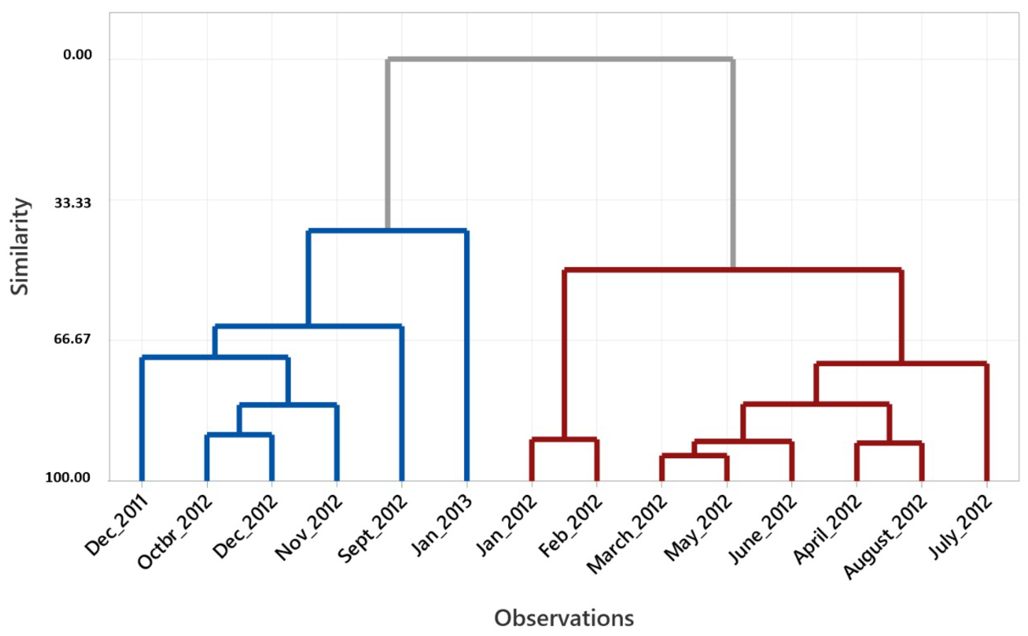
Next, we apply the hierarchical method with complete linkage to produce a dendrogram plot using |Minitab20.4| software as follows:

Figure 2. shows the claim data for December 2011, September to December 2012 and January 2013 are in the same group, say Group 1. On the other hand, claims data for the period January to August 2012 are in the second group, say Group 2.

Group 1 consist of 667 claims worth 5679 billion. Estimated total premiums received in those six months amounted to 602.3 billion. Besides that, in Group 2 there were 899 approved claims with an actual claim of 6021 billion. From January to August 2012, it is estimated that the total gross premiums received were worth 5773 billion. Based on this fact, we can conclude that the risks in Group 2 are greater than Group 1. In the next section, we will model the risk process for each of the groups formed.

3.2. Fitting Hawkes Process to Claim Payments Arrival

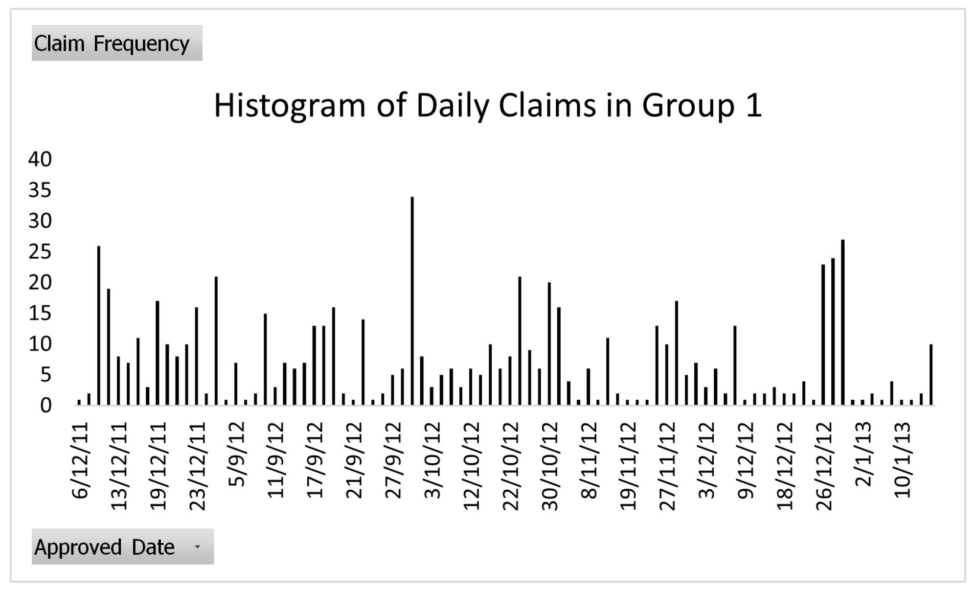
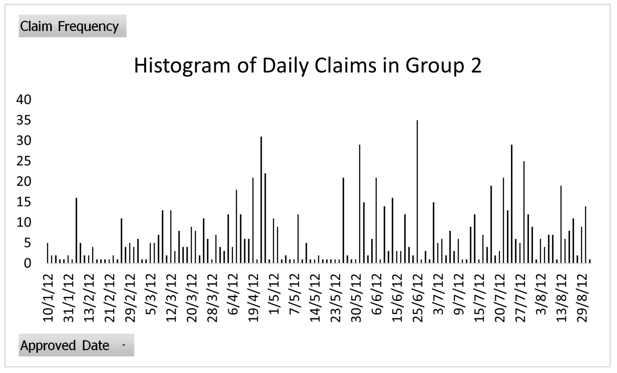
We would first draw the data histogram of how many claim payments there were in terms of days for Group 1 and Group 2, using Swishchuk et al. (2021)’s methodology, to determine whether the dataset could be incorporated into the Hawkes process or not with the help of Excel software. The results are shown in Figure 3 and Figure 4.

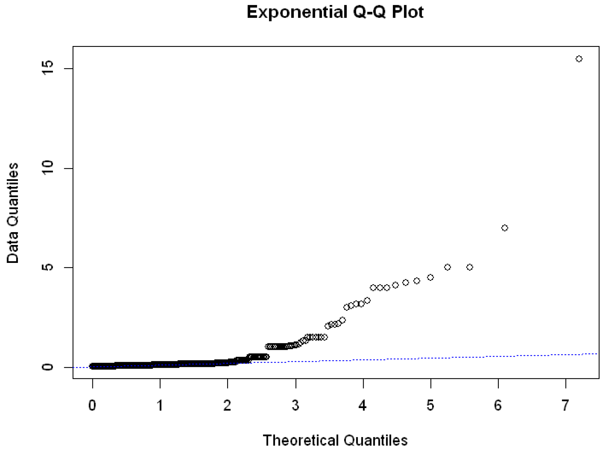
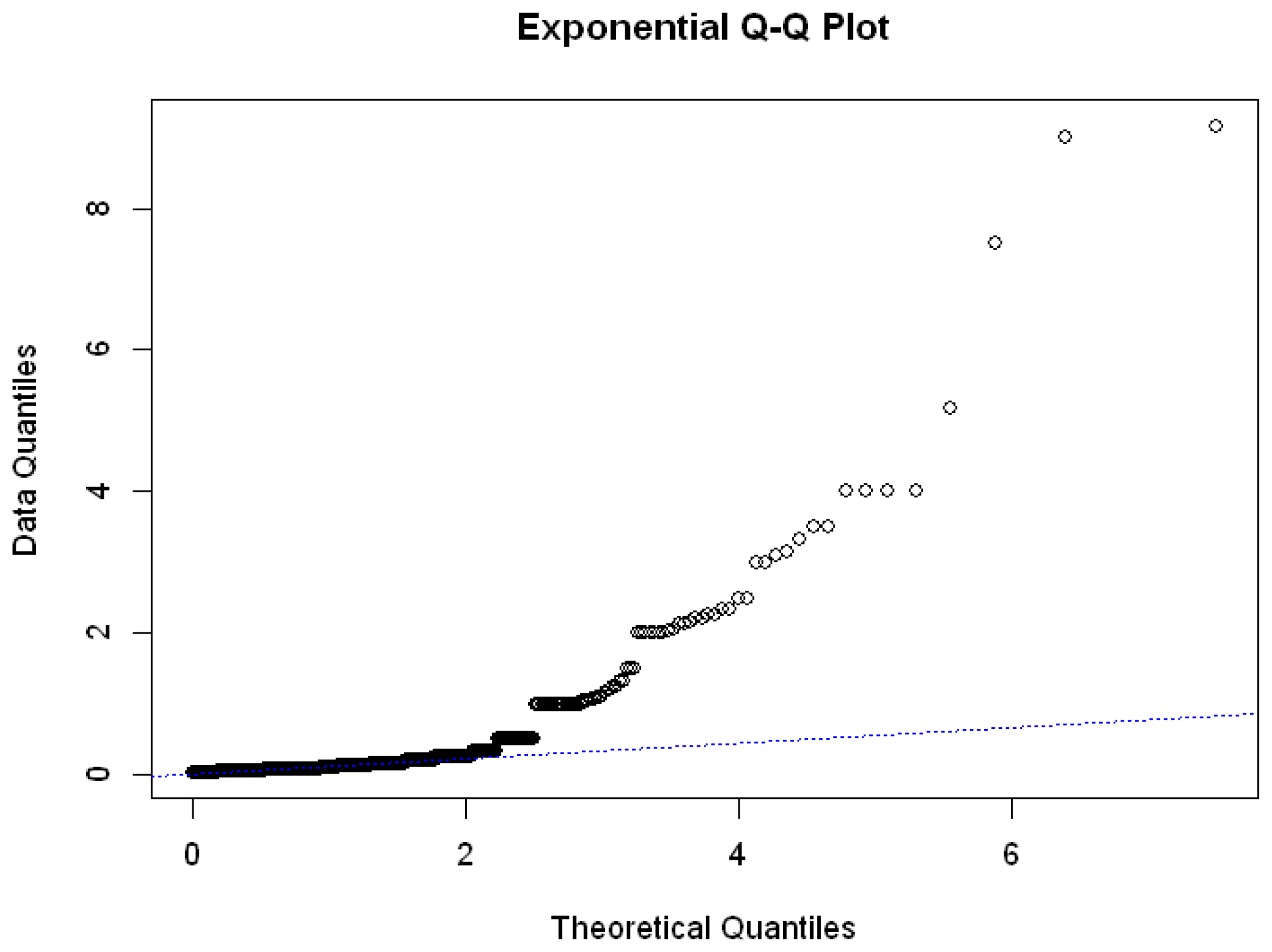
Since the Hawkes process is a simple point process, there should only be one event at a particular timestamp. We adjust the arrival time between two occurring events by distributing the occurrences evenly across the same day because our data timestamps are in days. After adjusting the arrival time, we plotted the interarrival time quantile beside the exponential distribution quantile using |R-4.10|software. The results are shown in Figure 5 and Figure 6.

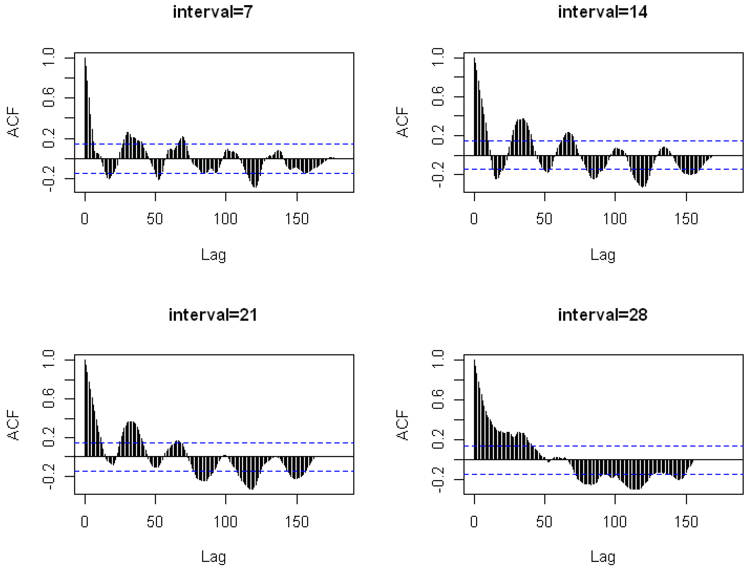
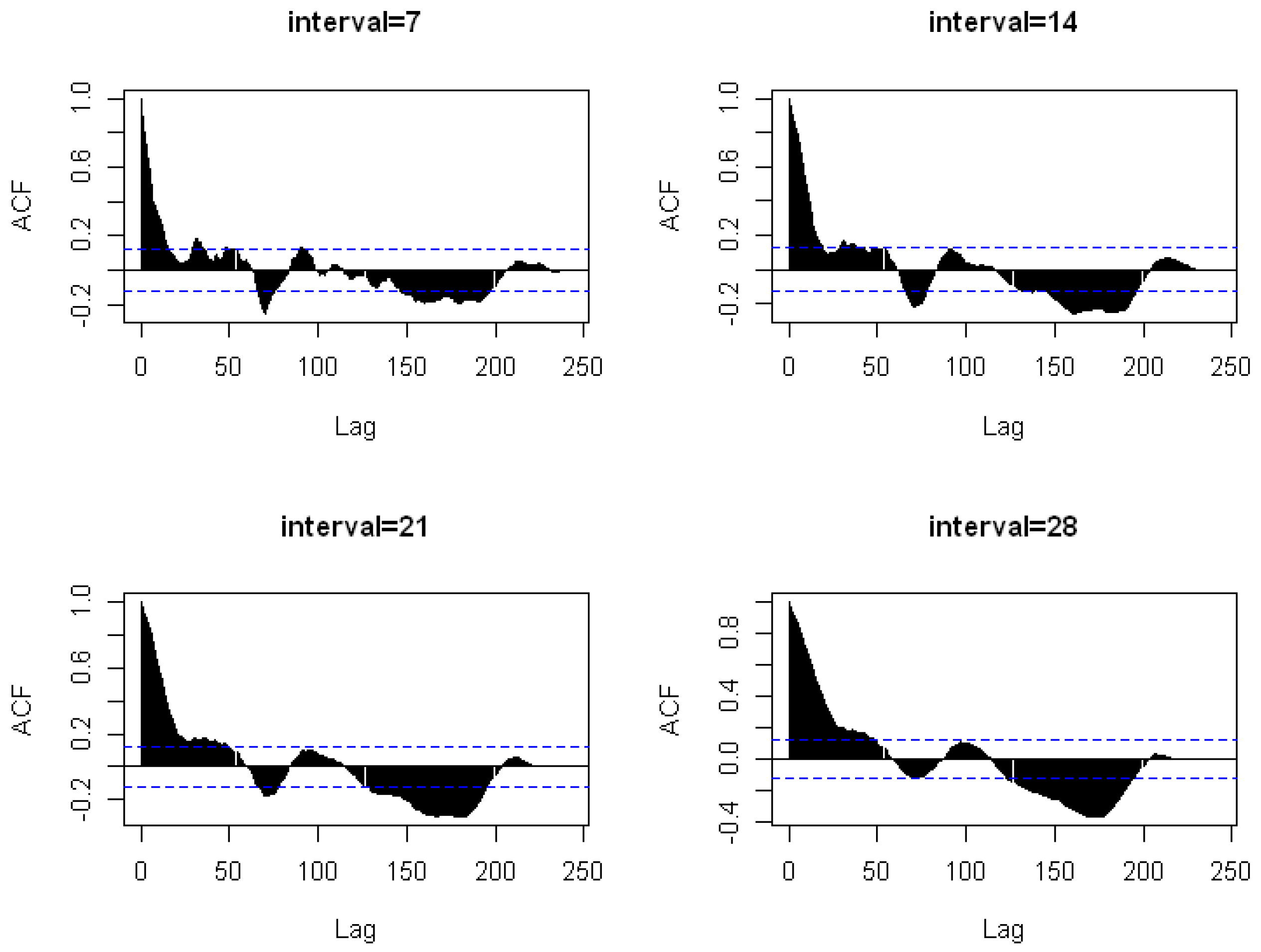
We could observe from Figure 5 and Figure 6 that the interarrival time did not fit the exponential distribution very well. It demonstrates that neither Group 1 nor Group 2’s data would match the Poisson distribution well. We then compute the autocorrelation plot of the interval of events with lengths of 7, 14, 21, and 28 using |R-4.10|software by repeating the procedures from Swishchuk et al. (2021) and Da Fonseca and Zaatour (2013). The results are shown in Figure 7 and Figure 8.

Based on the ACF plot above, we could conclude that the claim arrivals decay exponentially over time. Since the claim arrival data have a component of exponential decay, and exponential decay is one of the common choices for the excitation, then it is clear that the claim arrival data have self-excitation and exponential decay component, which is why we can use the Hawkes process fitting for the data.

The next step is to use the procedures from Shi and Odum Institute (2018) and use Peng (2003)’s PtProc R package to fit the data to the Hawkes process. The procedures are as follows:

• Simulate some starting positions by creating uniform random variables numbered from 1 to k for the starting points.
• Choose the starting point from those simulations that produce the theoretically predicted number of arrivals and variance of length 1 that are most similar to the observed ones. Say this number, c, and then the initial values for the next step are the triplet $({\lambda }_0=c,{\alpha }_0=c,{\beta }_0=c)$.
• With the observed time points, the exponential kernel, and the initial values of the parameters established by the previous step, create a Hawkes process using the |ptproc|function.
• Create a penalty for parameter values that are negative so that we can, hopefully, obtain estimates of the parameters that are positive.
• Call the |ptproc.fit()|function on the process we created in Step 3 to perform the estimation.
• Use (11) to compute the theoretical estimated number of arrivals for various interval duration.
• Examine the computed parameter’s theoretical variance for various interval duration using (12).

In this study, we choose $k=10$ and the length of arrival duration is 1, 7, 14 and 21 with the help of R software. The outcomes are displayed in

Table 1. Hawkes Estimated Parameters and their Empirical and Theoretical Estimated Number of Arrivals of Group 1.

Parameter	$\widehat{\mathit{\lambda }}$	$\widehat{\mathit{\alpha }}$	$\widehat{\mathit{\beta }}$	$\mathbb{E}\left[\widehat{\mathit{N}\left(1\right)}\right]$	$\mathbb{E}\left[\mathit{N}\right(1\left)\right]$
Estimated Value	0.5180797	2.522569	2.84654	3.625	4.552058

,

Table 2. Hawkes Estimated Parameters and their Empirical and Theoretical Estimated Number of Arrivals of Group 2.

Parameter	$\widehat{\mathit{\lambda }}$	$\widehat{\mathit{\alpha }}$	$\widehat{\mathit{\beta }}$	$\mathbb{E}\left[\widehat{\mathit{N}\left(1\right)}\right]$	$\mathbb{E}\left[\mathit{N}\right(1\left)\right]$
Estimated Value	0.7332754	3.024789	3.72142	3.684426	3.917172

,

Table 3. Comparison of Theoretical Variance of Poisson Process and Hawkes Process vs. Empirical Variance for Different Interval Length Time in Days of Group 1.

Interval Length	Theoretical Poisson Process Variance	Theoretical Hawkes Variance	Empirical Variance
1	4.224193	55.13359	39.58194
7	29.56935	1500.13435	407.49403
14	59.13870	3860.71443	865.84410
21	88.70805	6310.38508	1132.38060

and

Table 4. Comparison of Theoretical Variance of Poisson Process and Hawkes Process vs Empirical Variance for Different Interval Length Time in Days of Group 2.

Interval Length	Theoretical Poisson Process Variance	Theoretical Hawkes Variance	Empirical Variance
1	3.699588	34.09472	39.12012
7	25.89712	628.83392	300.68076
14	51.79423	1410.15783	845.94836
21	77.69135	2192.64436	1480.71268

.

As in Table 3 and Table 4, it is shown that the result of theoretical variance of Hawkes process is closer to the empirical variance than the result of theoretical variance of Poisson process so that the use of Hawkes process indeed improves the model fit.

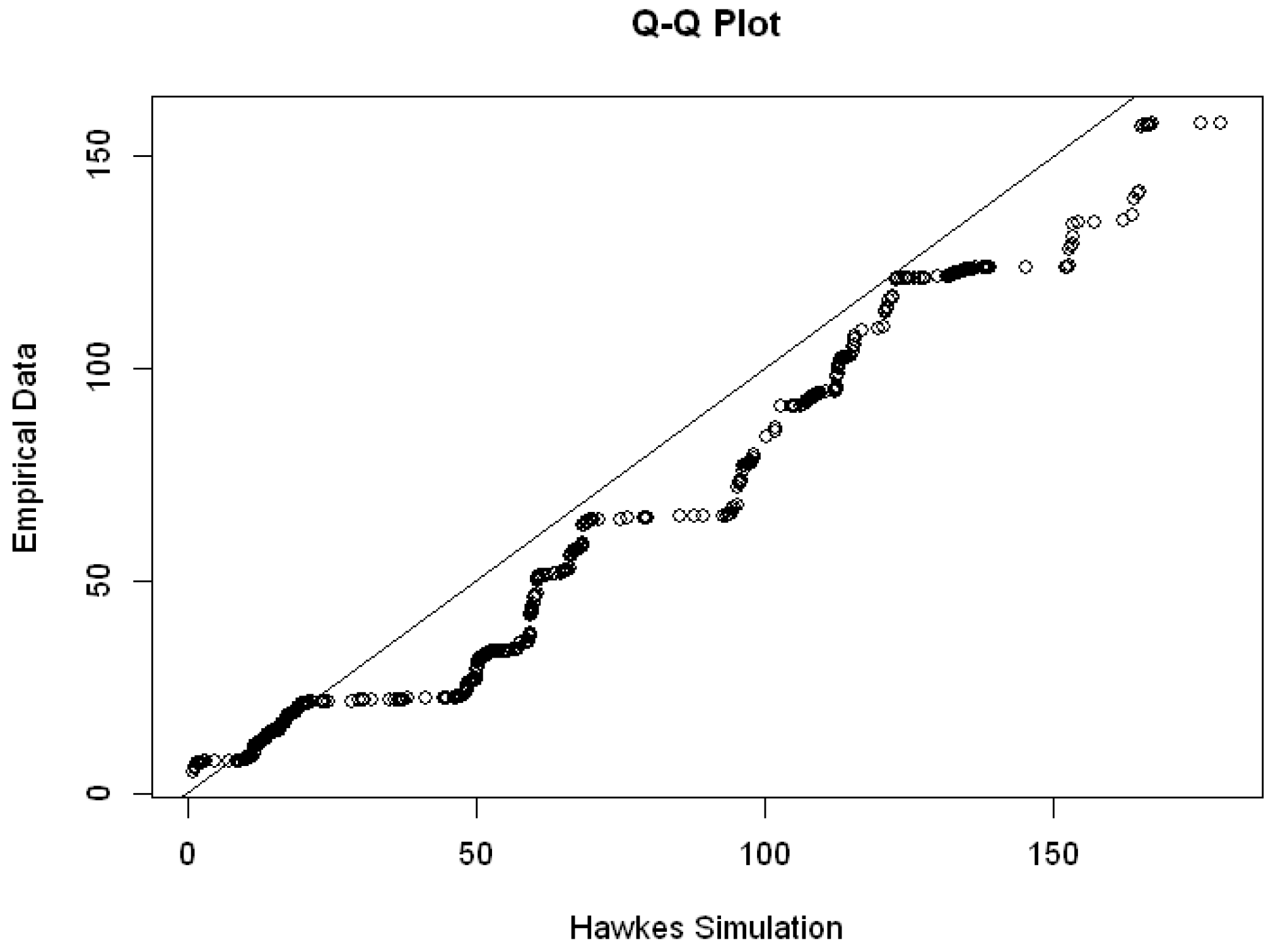
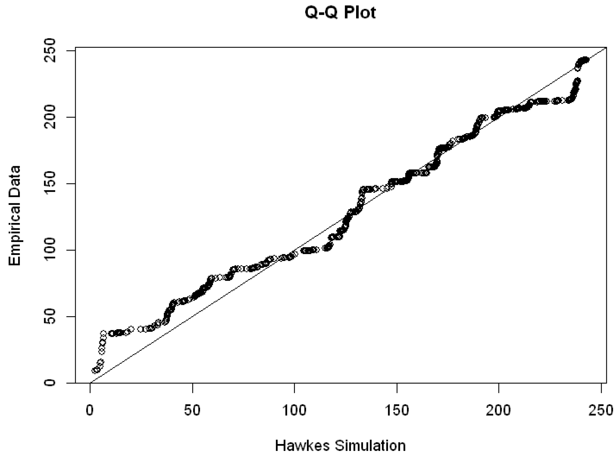
We then attempted to simulate a Hawkes process using Zaatour (2014)’s R package |hawkes|,to ensure that our data could be matched accurately with the Hawkes process of the determined parameters. The computations in the function are taken from Ogata (1981), which is referenced in Section 2.2.4. In Figure 9 and Figure 10, we then showed the simulation’s quantiles and the actual arrival time using R software. With the obtained parameters, we discovered that the Hawkes process could adequately replicate the empirical data for Group 2 data in Figure 10, but for Group 1 data in Figure 9, most of the points in the Q-Q plot are far below the line, it shows that the intensity of the Hawkes process is higher than the intensity of the empirical data.

3.3. Modeling the Claim Cost

For the claim cost, our empirical data (Y) shows that, for Group 1 we have the minimum claim cost of IDR 120,000, mean of IDR 8,514,808 and maximum (G) of IDR 157,782,000 and for Group 2 we have the minimum claim cost of IDR 50,000, mean of IDR 6,695,487 and maximum (G) of IDR 284,800,000. We use the empirical distribution function $\widehat{D}\left(G\right)$ as the distribution of the claim cost, and for that we have $\widehat{D}\left(G\right)=1$. We then make equally spaced boundaries g by dividing equally G by the number of states we want and count the state values $a\left(i\right)$ and the stationary distribution $p^{\star }$ for each state i. Using the formula in (20), (23) and (24), we developed our own syntax to calculate with the help of R software. The expected value was then obtained $a^{\star }$ that is the same as the expected value (mean) of the claim cost.

Table 5. 9-States Markov chain values for Group 1.

Parameter	Values
($g_1$; $g_2$; $g_3$; $g_4$; $g_5$; $g_6$; $g_7$; $g_8$; $g_9=G$)	(17,531,333; 35,063,667; 70,125,333; 87,656,667; 105,188,000; 122,719,333; 140,250,667; 157,782,000)
($p_1^{\star }$; $p_2^{\star }$; $p_3^{\star }$; $p_4^{\star }$; $p_5^{\star }$; $p_6^{\star }$; $p_7^{\star }$; $p_8^{\star }$; $p_9^{\star }$)	($0.931034483$; $0.023988006$; $0.013493253$; $0.007496252$; $0.008995502$; $0.002998501$; $0.004497751$; $0.004497751$; $0.002998501$)
($a\left(1\right)$; $a\left(2\right)$; $a\left(3\right)$; $a\left(4\right)$; $a\left(5\right)$; $a\left(6\right)$; $a\left(7\right)$; $a\left(8\right)$; $a\left(9\right)$)	(4,628,737; 22,900,401; 43,237,186; 66,041,056; 80,050,000; 100,400,000; 116,973,515; 124,194,000; 157,291,000)
$a^{\star }$	8,514,808
E(Y)	8,514,808

shows the result of the 9-States Markov chain we calculated for Group 1 and

Table 6. 4-states Markov chain values for Group 2.

Parameter	Values
($g_1$; $g_2$; $g_3$; $g_4=G$)	(71,200,000; 142,400,000; 213,600,000; 284,800,000)
($p_1^{\star }$; $p_2^{\star }$; $p_3^{\star }$; $p_4^{\star }$)	($0.979977753$; $0.016685206$; $0.00224694$; $0.001112347$)
($a\left(1\right)$; $a\left(2\right)$; $a\left(3\right)$; $a\left(4\right)$)	(4,418,278; 102,157,227; 154,791,000; 284,800,000)
$a^{\star }$	6,695,487
E(Y)	6,695,487

shows the result of the 4-states Markov chain we calculated for Group 2.

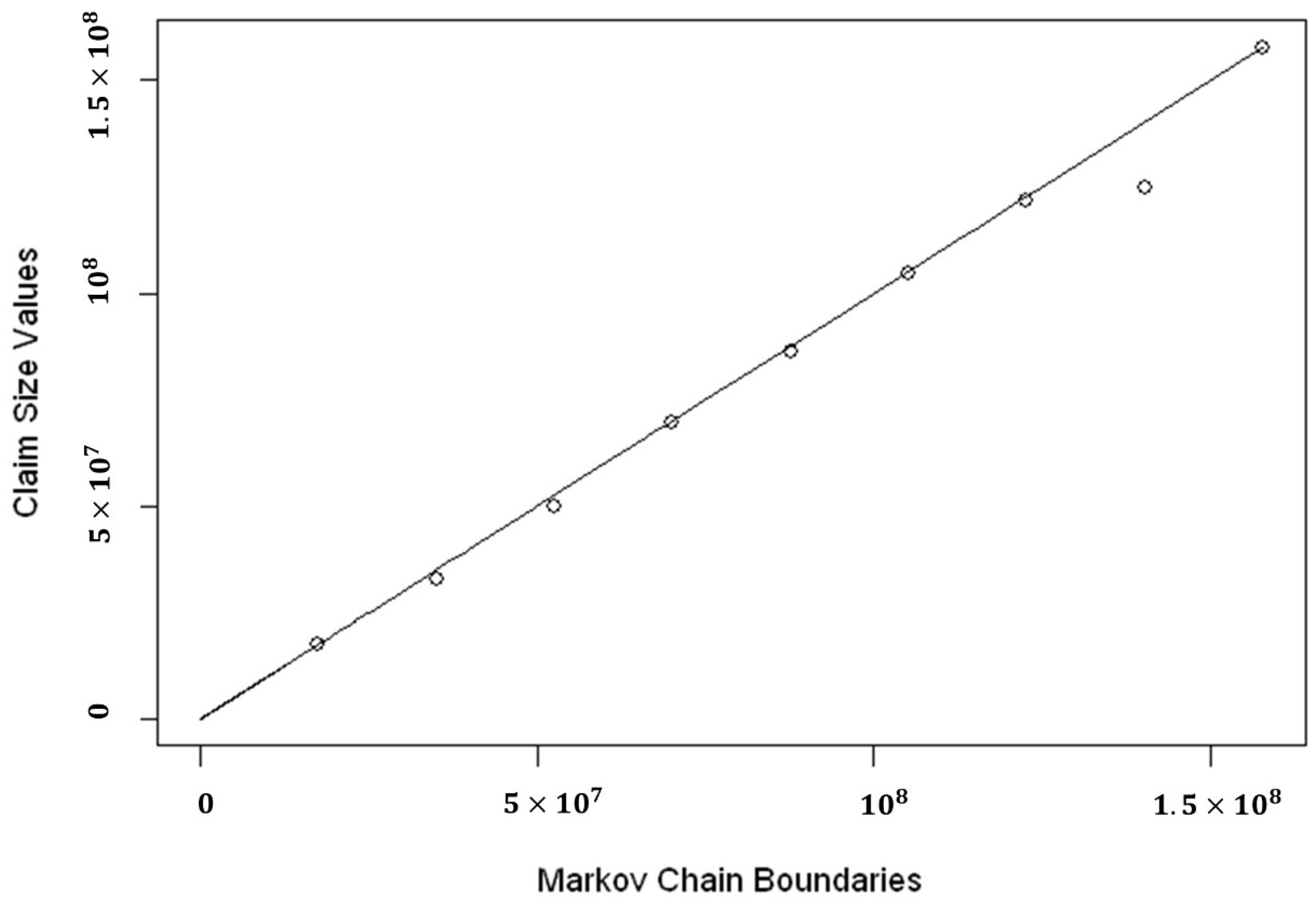
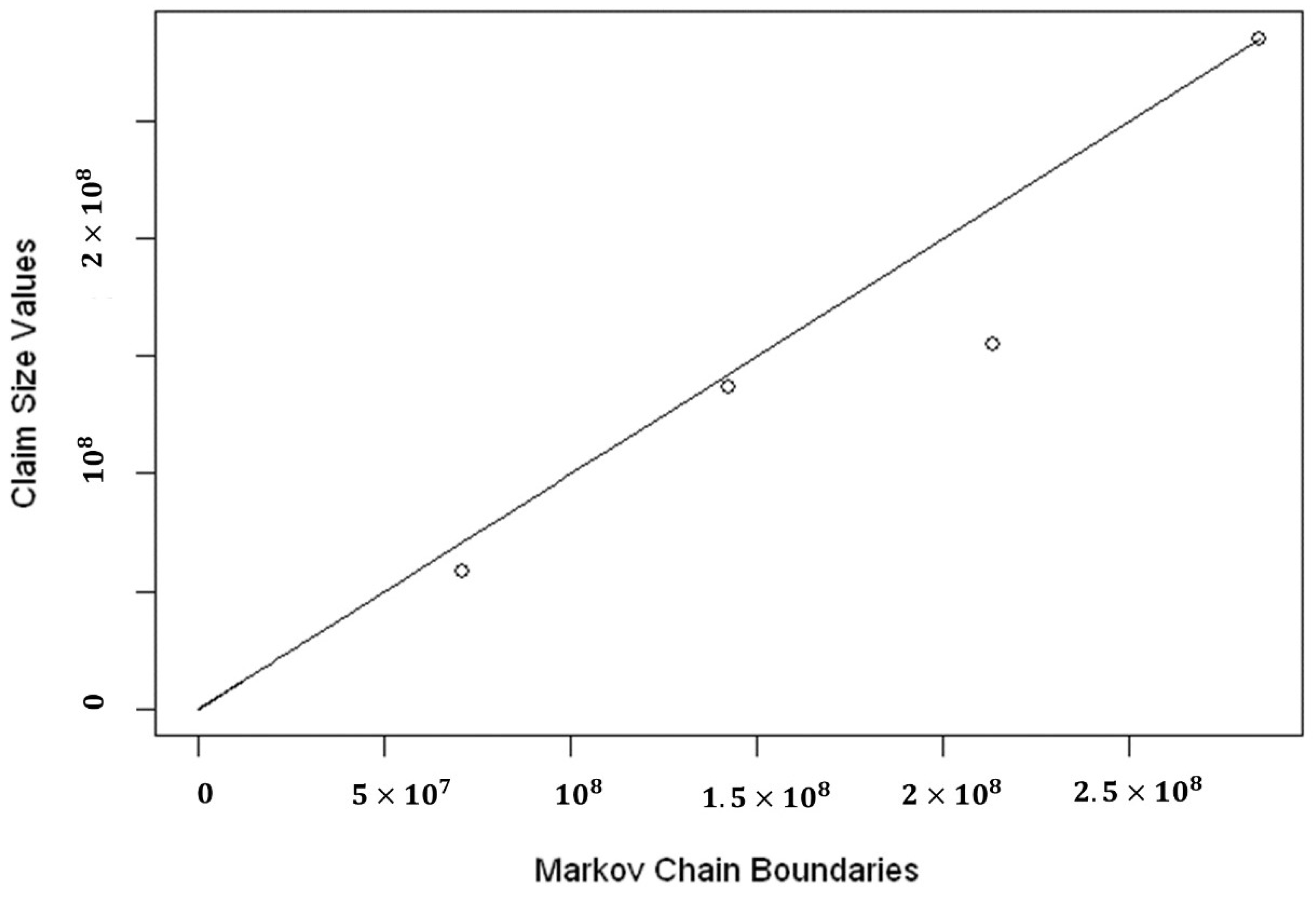
We must create an appropriate state space for the Markov chain to be irreducible in order to have a stationary distribution $p^{\star }$. For our data, we found that $N=9$ for Group 1 and $N=4$ for Group 2. This is due to the fact that, when we attempted to create 10 state spaces, we discovered that only one transitional probability of zero was produced, which rendered the Markov chain irreducible. Figures 12 and 13 show empirical distribution function and Q-Q plot of 9-states Markov chain for Group 1 while Figures 13 and 14  show that the 4-states Markov chain could replicate claim cost data in Group 2 quite well. We use R software to obtain the results in Figure 11, Figure 12, Figure 13 and Figure 14.

3.4. Risk Model Using General Compound Hawkes Processes

After determining that the Hawkes process and the time-continuous Markov chain could be used to represent the counting process and claim severity, we might attempt to describe the risk process using general compound Hawkes process. The initial capital, u, and continuous premium rate must be established before we can model the risk process. Please note that $c=max(\mathrm{50,387,867};\mathrm{34,095,590})=\mathrm{50,387,867}$. We use the maximum value of c that is calculated by Equation (31) so that it could cover the higher claims in both two groups.

We use the formula of Net Profit Condition and Premium Principle from (30) to determine the premium rate by taking $\theta =0.3$ as the safety loading. For the 9-States Markov chain, we obtain the $a^{\star }=$ 8,514,808. With the values we already calculated before, we obtain the premium rate, $c=max(\mathrm{50,387,867};\mathrm{34,095,590})=$ 50,387,867. For the initial capital, we consider the mean and maximum of the claim cost and decided that $u=\mathrm{mean}\left(\mathrm{claim}\mathrm{cost}\right)\times 70=\mathrm{596,036,550}$ is appropriate. For the 4-states Markov chain, we obtain the $a^{\star }=$ 6,695,487. With the values we already calculated before, we obtain the premium rate $c=$ 28,850,114. For the initial capital, we consider the mean and maximum of the claim cost and decided that $u=\mathrm{mean}\left(\mathrm{claim}\mathrm{cost}\right)\times 10=\mathrm{66,954,873}$ is appropriate. In the context of contrasting the fit of Hawkes models with exponential kernels to empirical data, Zhang (2016) proposes a metric, $\widehat{S}$ and $\widehat{F}$ as the following:

$$\widehat{S}\left(K\right)=\frac{1}{K}\sum _{i=1}^L\frac{max\left({\widehat{R}}_i\left(t\right)\right)-min\left({\widehat{R}}_i\left(t\right)\right)}{max\left(R\right(t\left)\right)-min\left(R\right(t\left)\right)}.$$

(32)

$$\widehat{F}\left(K\right)=\frac{1}{K}\sum _{i=1}^K\frac{{\widehat{R}}_i\left(T\right)}{R\left(T\right)}.$$

(33)

where ${\widehat{R}}_i\left(t\right)$ stands for the simulated risk processes, $R\left(t\right)$ stands for the benchmark of empirical process and K stands for the number of simulated paths.

Using the calculated u and c, we then derive the empirical risk process and simulate $L=1000$ paths of risk process with arrival time following Hawkes process with parameters for group 1 are $\widehat{\lambda }=0.5180797,\widehat{\alpha }=2.522569$ and $\widehat{\beta }=2.84654$ and parameters for group 2 are $\widehat{\lambda }=0.7332754,\widehat{\alpha }=3.024789$ and $\widehat{\beta }=3.72142$. The claim severity in groups 1 and 2, respectively, follows a 9-state Markov chain and a 4-state Markov chain. Then, we simulate with the same value of arrival time generated by Hawkes simulation from |hawkes|library in R and randomly generated Markov chain states simulations. 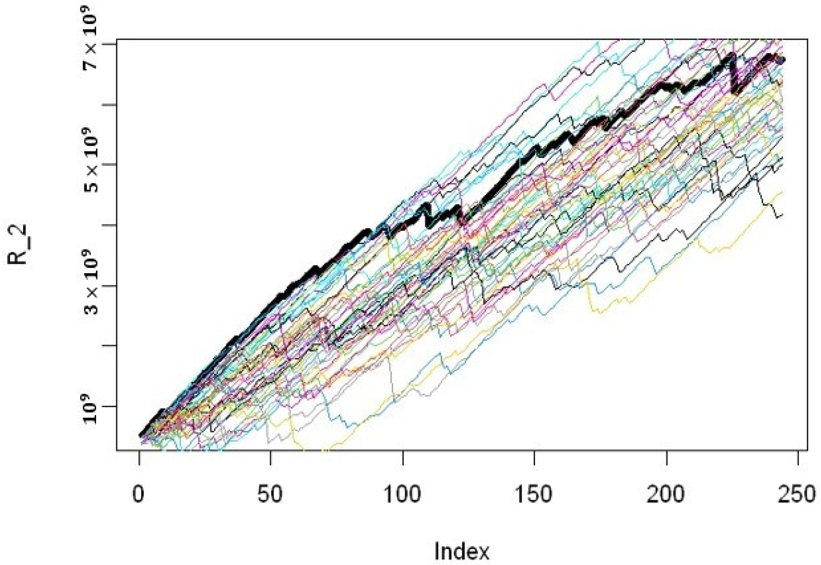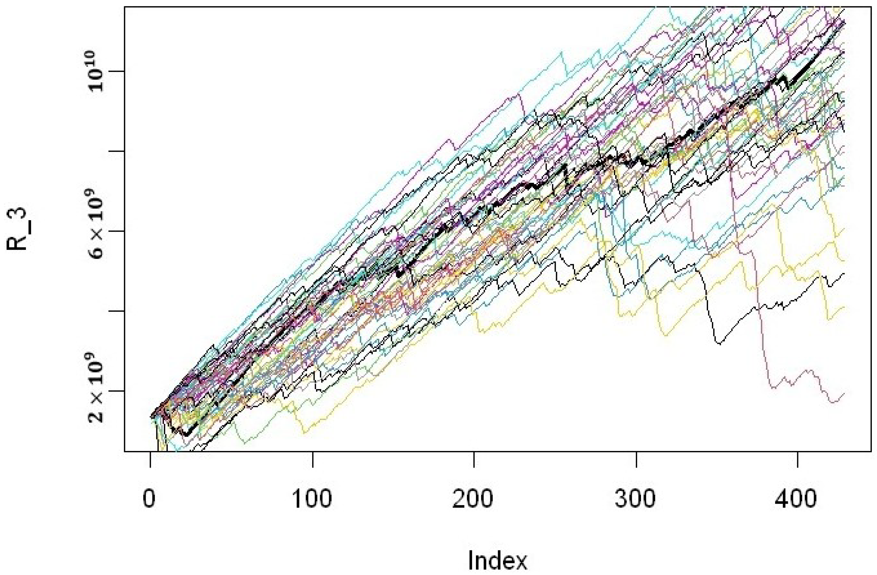Figure 15, Figure 16 and Figure 17 shows the plot of the empirical risk process and the first 50 simulations. We use R software to obtain the figures. We could see from the plot that the simulations adequately represented the empirical process. Then we use the formulas from Swishchuk et al. (2021) to compute the comparison of fluctuation over time and at time $T=184$ days for Group 1 and $T=244$ days for Group 2. Then, we can calculate the average historical insurance reserve with the help of R software. We obtain the results in

Table 7. The result of the comparison between an empirical risk process and simulations of the general compound Hawkes process at time $T=184$ in Group 1.

Parameter	Method	Values
$\widehat{S}\left(K\right)$	metric	0.9367684
$\widehat{F}\left(K\right)$	metric	0.6978924
$R\left(T\right)$	empirical	4,443,471,513
$E\left[R\right(T\left)\right]$	simulations	891,786,394
$\sqrt{Var\left[R\right(T\left)\right]}$	simulations	26,348,096

,

Table 8. The result of the comparison between an empirical risk process and simulations of the general compound Hawkes process at time $T=244$ in Group 2.

Parameter	Method	Values
$\widehat{S}\left(K\right)$	metric	0.9784721
$\widehat{F}\left(K\right)$	metric	0.9650283
$R\left(T\right)$	empirical	6,744,080,615
$E\left[R\right(T\left)\right]$	simulations	509,061,428
$\sqrt{Var\left[R\right(T\left)\right]}$	simulations	24,506,352

and

Table 9. Result of Insurance reserve comparison between period in each Groups.

	Group 1	Group 2	All Data
Average historical insurance reserve	38,161,865	25,635,635	31,020,743

.

3.5. Discussion

This study reveals that a high claim period and low claim period have quite different characteristics in terms of claims volatility. As a result of these differences in characteristics, the required reserves differ significantly. Table 9 shows a considerable difference between the first group, which occurs during the high claim period, and the second group, which is dominated by the low claim period, in terms of the average historical insurance reserve.

In addition, when compared to earlier studies in risk theory that employed the Hawkes process, this study can also help in the development of a novel technique for concurrently classifying and estimating insurance reserves that entails grouping risks with comparable loss potential and imposing new various manual rates to account for variations in loss potential within the groupings.

For further research, for instance, longitudinal data analysis can be used to model the risk with the Hawkes process from claim data that contains observations about different cross sections across time.

4. Conclusions

The Hawkes processes are incredibly intriguing representations of reality. Since many of the common probability models are Markovian, they ignore the process’s history. The Hawkes processes are built on the foundation that history matters, which helps to explain why they are used in such a wide variety of applications. The use of the Hawkes process in estimating the calculation of insurance reserves can be used as a good alternative method because of its ability to anticipate behaviors that have spread throughout reserves over time. Claims from the past typically result in higher reserves and new claims have a bigger impact on reserves than outdate claims. The Hawkes process, which primarily exhibits self-excitation and exponential decay, is well suited to describing these occurrences.

The clustering method, which is essentially a type of unsupervised learning method, allows us to categorize risk processes based on claim frequency domain. This involves grouping risks with similar loss potential and imposing a reserve estimation to account for variations in loss potential within the groupings.

This approach may have consequences for changes in the insurer’s perspective that have not yet been taken into consideration: the potential for variations between groups in the frequency domain. Finding the risk criteria that divide risks into groups with comparable expected loss experiences is therefore considered to be a step in applying this strategy.

References

- Bessy-Roland, Yannick, Alexandre Boumezoued, and Caroline Hillairet. 2021. Multivariate Hawkes process for cyber insurance. Annals of Actuarial Science 15: 14–39. [Google Scholar] [CrossRef]
- Cheng, Zailei, and Youngsoo Seol. 2020. Gaussian approximation of a risk model with stationary Hawkes arrivals of claims. Methodology and Computing in Applied Probability 22: 555–71. [Google Scholar] [CrossRef]
- Da Fonseca, José, and Riadh Zaatour. 2013. Hawkes process: Fast calibration, application to trade, clustering and diffusive limit. Journal of Futures Markets 34: 548–79. [Google Scholar] [CrossRef]
- Filimonov, Vladimir, and Didier Sornette. 2015. Apparent criticality and calibration issues in the Hawkes self-excited point process model: Application to high-frequency financial data. Quantitative Finance 15: 1293–314. [Google Scholar] [CrossRef]
- Gao, Xuefeng, and Lingjiong Zhu. 2017. Limit theorems for Markovian hawkes processes with a large initial intensity. Stochastic Processes and their Applications 128: 3807–39. [Google Scholar] [CrossRef]
- Hartigan, John A. 1975. Clustering Algorithms. New York: Wiley-Interscience. [Google Scholar]
- Hawkes, Alan G. 1971. Spectra of some self-exciting and mutually exciting point processes. Biometrika 58: 83–90. [Google Scholar] [CrossRef]
- Jeong, Himchan, and Bin Zou. 2022. A Dynamic Credibility Model with Self-Excitation and Exponential Decay (9 September 2022). Proceedings of the 2022 Winter Simulation Conference. Available online: https://ssrn.com/abstract=4214889 (accessed on 5 May 2022).
- Johnson, Richard A., and Dean W. Wichern. 2009. Applied Multivariate Statistical Analysis. New York: John Wiley & Sons, pp. 680–95, chp. 12, section 12.3. [Google Scholar]
- Kaufman, Leonard, and Peter J. Rousseeuw. 1990. Finding Groups in Data: An Introduction to Cluster Analysis. New York: John Wiley & Sons, Inc. ISBN 9780471878766. [Google Scholar]
- Laub, Patrick J., Thomas Taimre, and Phillip K. Pollett. 2015. Hawkes processes. arXiv arXiv:1507.02822. [Google Scholar]
- Lefèvre, Claude, and Phillipe Picard. 2006. A nonhomogeneous risk model for insurance. Computers and Mathematics with Applications 51: 325–34. [Google Scholar] [CrossRef]
- Lundberg, Filip. 1903. I. Approximerad Framstallning af Sannolikhetsfunktionen: II. Aterforsakring af kollektivrisker. Uppsala: Almqvist Wiksell. [Google Scholar]
- Ogata, Yosihiko. 1981. On Lewis’ simulation method for point processes. IEEE Transactions on Information Theory 27: 23–31. [Google Scholar] [CrossRef]
- Ogata, Yosihiko. 1999. Seismicity Analysis through Point-process Modeling: A Review. Pure and Applied Geophysics 155: 471–507. [Google Scholar] [CrossRef]
- Peng, Roger D. 2003. Multi-dimensional Point Process Models in R. Journal of Statistical Software 8: 1–27. [Google Scholar] [CrossRef]
- Răducan, Anişoara Maria, Raluca Vernic, and Gheorghiţă Zbăganu. 2015. On the ruin probability for nonhomogeneous claims and arbitrary inter-claim revenues. Journal of Computational and Applied Mathematics 290: 319–33. [Google Scholar] [CrossRef]
- Romaniuk, Maciej. 2019. Simulation-Based Analysis of Penalty Function for Insurance Portfolio with Embedded Catastrophe Bond in Crisp and Imprecise Setups. In Information Systems Architecture and Technology: Proceedings of 39th International Conference on Information Systems Architecture and Technology-ISAT 2018. Advances in Intelligent Systems and Computing. Cham: Springer, vol. 854. [Google Scholar] [CrossRef]
- Shi, Feng, and Odum Institute. 2019. Learn About the Hawkes Process in R With Data From the DJIA 30 Stock Time Series (2018). London: SAGE Publications Ltd. [Google Scholar] [CrossRef]
- Stabile, Gabriele, and Giovanni Luca Torrisi. 2010. Risk processes with non-stationary Hawkes claims arrivals. Methodology and Computing in Applied Probability 12: 415–29. [Google Scholar] [CrossRef]
- Swishchuk, Anatoliy. 2017. Risk model based on general compound Hawkes processes. arXiv arXiv:1706.09038. [Google Scholar]
- Swishchuk, Anatoliy, Rudi Zagst, and Gabriela Zeller. 2020. Hawkes Processes in Insurance: Risk Model, Application to Empirical Data and Optimal Investment. Insurance Mathematics and Economics 101: 107–24. [Google Scholar] [CrossRef]
- Zaatour, Riadh. 2014. |hawkes|:Hawkes process simulation and calibration toolkit. R package version 0.0.4. Available online: https://CRAN.R-project.org/package=hawkes (accessed on 5 May 2022).
- Zhang, Changyong. 2016. Modeling high frequency data using hawkes processes with power-law kernels. Procedia Computer Science 80: 762–71. [Google Scholar] [CrossRef]
Figure 1.
Hartigan Index plot to determine the number of groups from Indonesian Insurance data.
Figure 2.
The Dendrogram plot shows that there are two groups of claim data formed.
Figure 3.
Histogram of Numbers of Claim Payments in Group 1.
Figure 4.
Histogram of Numbers of Claim Payments in Group 2.
Figure 5.
Exponential Q-Q plot of interarrival time between 2 occurring claims in Group 1.
Figure 6.
Exponential Q-Q plot of interarrival time between 2 occurring claims in Group 2.
Figure 7.
Autocorrelation (ACF) plot of interval length 7, 14, 21 and 28 in Group 1.
Figure 8.
Autocorrelation (ACF) plot of interval length 7, 14, 21 and 28 in Group 2.
Figure 9.
Q-Q plot of arrival time simulated by Hawkes process with parameters and empirical data of Group 1.
Figure 10.
Q-Q plot of arrival time simulated by Hawkes process with parameters and empirical data of Group 2.
Figure 11.
Distribution function of empirical data and 9-states Markov Chain for Group 1 [].
Figure 12.
QQ-plot of Markov Chain claim boundaries and empirical claims in the boundaries for Group 1.
Figure 13.
Distribution function of empirical data and 4-states Markov Chain for Group 2 [].
Figure 14.
QQ-plot of Markov Chain claim boundaries and empirical claims in the boundaries for Group 2.
Figure 15.
Plot of empirical risk process (bold line) and 50 simulations of the general compound Hawkes process in Group 1.
Figure 16.
Plot of empirical risk process (bold line) and 50 simulations of the general compound Hawkes process in Group 2.
Figure 17.
Plot of empirical risk process (bold line) and 50 simulations of the general compound Hawkes process for all data.