Trading Binary Options Using Expected Profit and Loss Metrics

Abstract

Trading in binary options is discussed using an approach based on expected profit (EP) and expected loss (EL) as metrics of reward and risk of trades. These metrics are reviewed and the role of the EL/EP ratio as an indicator of quality of trades, taking risk tolerance into account, is discussed. Formulas are derived for the EP and EL of call and put binaries assuming that the price of the underlying asset follows a geometric Brownian motion. The results are illustrated with practical data from the Nadex trading platform. The Black–Scholes notion of implied volatility is extended to wider notions of implied drift and volatility of the price process of the underlying asset. Illustrations show how these notions can be used to identify attractive binary trades, taking anticipated price movement into account. The problem of selecting portfolios of call and put binary options which maximize portfolio EP while constraining the portfolio EL to satisfy risk tolerance and diversification requirements, is formulated and solved by linear programming. This is also illustrated with the Nadex data under various scenarios.

1. Introduction

The notions of risks and rewards are important factors driving financial markets. Here is an illustrating quote: “In the near term, investors are still digesting, still assessing the risks and rewards as a result of the Ukraine invasion and the implications of Western sanctions on Russia”, Yang (2022). While these events have many geopolitical implications, for investors the most important issue is to assess the resulting financial risks and rewards. Assessing risks and rewards in a trading context requires actionable metrics—a more demanding task than delivering broad intuitive moral or political judgements.

This paper is concerned with trading in binary options. In principle, binary options are among the simplest financial assets to trade in. There are two forms of binary options: “cash-or-nothing” and “asset-or-nothing”. In this paper we treat only the simplest of the two, namely the cash-or-nothing binaries. On expiry this binary call option pays the trader a fixed amount of money if the underlying asset price is above the strike price and nothing at all otherwise. The corresponding binary puts differ only in that the pay-outs happen when the price of the underlying is below the strike price, rather than above. Our primary focus is on the use of expected profit (EP) and expected loss (EL) as suitable actionable risk and reward metrics in this context. For brevity, we refer to use of these metrics as the EPEL approach. The precise meaning of these terms is defined and discussed in Section 3, but first, some background on option pricing theory is presented.

The formal theory of pricing options in general started with the introduction of the Black–Scholes (BS) formulas for pricing options; see Black and Scholes (1973). The BS approach chooses a plausible probability model for the price process of the underlying instrument, specifying conditions which allow execution of a replicating portfolio to eliminate arbitrage possibilities for the parties involved in the option trade. This leads to the celebrated so-called “risk-neutral” BS pricing formulas. A typical model for the price process is the geometric Brownian motion (GBM). Section 2 below reviews the BS formulas for binary options.

The practicality of the BS approach to option pricing has been questioned by many authors; see e.g., Derman and Taleb (2005), Jankova (2018) or Hurvich (2021). While risk-neutrality in the BS sense, may be a reasonable feature to have, it does not provide the parties involved in an option trade explicit information on possible profits and losses that may be expected from the trade. The adage “to make profits, you must take risk” usually applies in trading. If all parties are risk-neutral, what would motivate them to trade? This is where the EPEL approach provides useful information, complementing that of the BS pricing formulas. Section 3 below provides the background of the EPEL approach to trading in general and also derives the required formulas for the EP and the EL when specialized to trading binary options.

The book of Cofnas (2016) provides an excellent introduction to trading binary options, together with sound practical strategies and advice to traders. However, the treatment is somewhat informal from a statistical technical perspective. Measuring profitability is emphasized and illustrated numerically, but measuring risk is not treated on the same level. As will be pointed out in Section 3 and subsequent sections below, treating both reward and risk metrics simultaneously is a particularly appealing aspect of the EPEL approach.

Section 4 below provides an extensive illustration of binary trading using practical data. The exact details of trading in binary options differ on different exchanges and platforms (of which there are many). Some forms of binary trading have a reputation of possible fraudulence. Warnings to this effect were issued by the US Securities Exchange Commission (SEC); see e.g., https://www.sec.gov/files/ia_binary.pdf (accessed on 21 October 2022). We use the reputable US platform Nadex (Nadex.com 2022) (https://platform.nadex.com/npwa/#/login, accessed on 8 February 2022), regulated by the Commodity Futures Trading Commission. Both the BS and the EPEL approaches are illustrated using data from the Nadex platform. Calculation and use of the BS implied volatilities in the binary context are discussed. A novel method is introduced to estimate a new type of implied volatility that represents a consensus volatility value, based on the option prices over all strikes. This is an alternative way to use the BS formulas to find mispriced options. An analogous method based on the Nadex probability assessments yields implied drift and volatility parameters of the price process of the underlying asset. The process is found to strongly resemble a GBM model. This links the Nadex trading information to the EP and EL formulas of Section 3. With these EPEL links, the quality of trades available to the trader can be evaluated, allowing for various views the trader may have on the possible price movements of the underlying asset. This helps the trader to make trading decisions based on reward and risk tolerance considerations. The illustration demonstrated that the EPEL provides the trader with more useful trading information than that of the BS formulas.

Section 5 below deals with option selection issues. Traders are typically faced with selecting from among many possible choices when trading options: what types of options to select, what assets underlying the options to choose, what strike levels to use, whether to sell or buy, and how to allocate capital among these items. Section 5 formulates these as optimal portfolio selection problems, but now using EPEL on the level of portfolios of binaries, rather than individual binaries. This is a remarkable contribution of the paper, namely that the EPEL approach can deal effectively with both individual option evaluation and option portfolio selection. A further strong contribution is that optimal portfolios can be found by solving linear programming problems. Section 6 provides practical illustrations of such portfolio solutions, again using data from the Nadex platform.

Section 7 concludes with a brief review of the contents of the paper, followed by a discussion of important remaining matters for future research.

2. Black-Scholes Formulas for Call and Put Binary Options

Some notation and assumptions need to be introduced. Let $S_0$ denote the price of the underlying asset at the start of the trading period. Moreover, denote the strike price of the option on expiry of the period by $K$ and the cash pay-out on expiry by $Q$ units for each of a successful call or put binary. Without loss of generality, we assume that the duration of the period to expiry is 1 time unit. We only treat binary options of European type. Then, with $S_1$ denoting the price of the underlying at expiry, the pay-out of the call binary is $Q$ if $S_1>K$ and 0 otherwise. For a put binary, the pay-out is $Q$ if $S_1\le K$ and 0 otherwise.

The BS formulas for pricing of cash-or-nothing binary options, can be found from many sources, among which Hull (2006). With Φ denoting the cumulative distribution function (CDF) of the standard normal distribution, the BS prices of the binary call and put options are

$$C_{BS}=Q{e}^{-r}\Phi \left(d\right) \mathrm{and} P_{BS}=Q{e}^{-r}\Phi \left(-d\right) \mathrm{where} d=[\log (S_0/K)+(r-{\sigma }^2/2)]/\sigma$$

(1)

Here r denotes the risk-free interest rate, σ denotes the volatility of the log-price of the underlying asset, and we assume no dividends are in play. The risk-neutral model on which these formulas are based is that the price of the underlying asset follows a GBM process with volatility σ and with drift parameter $\mu =r-{\sigma }^2/2$. Note the formula

$$C_{BS}+P_{BS}=Q{e}^{-r}$$

(2)

which simply states that buying one call binary and one put binary is equivalent to the discounted value of certainly receiving Q units of cash at expiry. This has nothing to do with the way we arrive at the two prices $C_{BS}$ and $P_{BS}$ and may be regarded as a necessary consistency condition to be satisfied by any choice of the prices of a binary call and a binary put on some underlying asset. This may not be true if trading costs are involved. To focus on the EPEL approach in its simplest form, zero trading cost is assumed in this paper.

3. The EPEL Approach for Call and Put Binary Options

Given the BS prices of binary options, do trading at these prices lead to good results? The EPEL approach can shed light on this question by supplying additional useful reward and risk information to the trader. This is discussed in this section. Before specializing to the binary option context, we first review the main aspects of the EPEL approach to judging the quality of prospective trades in more general contexts.

Denote the profit and loss (P&L) of a typical trade by the random variable $X$, distributed according to some probability measure $\mathbb{P}$ and let $\mathbb{E}$ denote expectation under $\mathbb{P}$. If $X$ > 0, the trade results in a profit. Hence the size of the profit of the trade is the positive part of $X$, denoted by $X^{+}=$ max {$X$,0}. Similarly, if $X$ < 0 the trade results in a loss and the size of the loss is the negative part of $X$, denoted by $X^{-}=\max \left\{-X,0\right\}$. Then $\mathbb{E}{X}^{+}$ and $\mathbb{E}{X}^{-}$ are the expected profit (EP) and expected loss (EL) of the trade, respectively. They are the reward and risk metrics of the EPEL approach. They are both expressed in the same monetary terms. This makes them directly comparable. For example, if a trade has an EL that is less than one-fifth of its EP, then it is intuitively clear that this would be an attractive trade, even if the trader has low risk tolerance (or appetite).

More generally, if the EP and EL of a trade satisfies the risk constraint $\mathbb{E}{X}^{-}\le \lambda \mathbb{E}{X}^{+}$, then it would be acceptable to a trader operating at a risk tolerance level $\lambda .$ Here $\lambda$ is a number between 0 and 1. If the risk constraint only held for $\lambda >1$, then the risk of the trade may be larger than its reward. This would typically not be attractive to a trader—hence the restriction $\lambda \le 1$. Further, on the border, if the risk constraint holds only with $\lambda =1$, then the risk may equal the reward, i.e., $\mathbb{E}{X}^{+}=\mathbb{E}{X}^{-}$. Such a trade is neither attractive nor unattractive and may be said to be quality-neutral. A trader with $\lambda$ just below to 1, may be described as risk tolerant, whereas a trader with $\lambda$ smaller, is less risk tolerant (or more risk averse). The risk constraint $\mathbb{E}{X}^{-}\le \lambda \mathbb{E}{X}^{+}$ can be written in terms of the EL/EP ratio in the form $\mathbb{E}{X}^{-}/\mathbb{E}{X}^{+}\le \lambda$. A trader operating at a risk tolerance level $\lambda$, looks for trades whose EL/EP ratio is below $\lambda$. The EL/EP ratio may thus be thought of as an indicator, expressing the quality or attractiveness of a trade.

To summarize, the EPEL approach follows three steps to judge a prospective trade. Firstly, find the reward to be expected from the trade—its EP expressed by the formula $\mathbb{E}{X}^{+}$. Second, decide on the risk tolerance level $\lambda$ at which to operate—the maximal fraction of the reward allowed to cover the risk of the trade. Third, verify that the risk constraint holds, i.e., that $\mathbb{E}{X}^{-}\le \lambda \mathbb{E}{X}^{+},$ in which case, proceed with the trade.

The metrics $\mathbb{E}{X}^{+}$ and $\mathbb{E}{X}^{-}$ are related to the Omega ratio of Keating and Shadwick (2002). Taking the threshold (or reference level) in the Omega ratio as 0 and applying it to the trade set-up above, the Omega ratio may be written as $\mathbb{E}{X}^{+}/\mathbb{E}{X}^{-}$; see e.g., Bernard et al. (2019). The Omega ratio was originally introduced as a performance measure for portfolio returns, aimed at improving on other ratios such as those of Sharpe (1966) and the Sortino ratio; see e.g., Sortino and Van Der Meer (1991) or Sortino and Price (1994). These ratios are popular performance metrics in diverse portfolio applications; see e.g., Platanakis and Urquhart (2019). However, the applications below to binary options trading, makes some of them less suitable. The Sharpe ratio uses the expectation and variance (or standard deviation) of return as reward and risk metrics, in line with the mean-variance portfolio theory of Markowitz (1968). The use of variance as risk metric, does not distinguish between (good) returns above the mean and (bad) returns below the mean; see e.g., Estrada (2006). Moreover, it does not take features such as skewness of the probability distribution of returns into account. This is particularly acute in our binary trading context. It will be shown in the sections below that the distribution of the P&L in the binary context is discrete with only two mass points, one below 0 and one above 0, while their probabilities may be very different. The Sharpe ratio does not cater for such cases.

The Sortino ratio uses the expected return as the reward metric, but to improve on the Sharpe ratio, it bases its risk metric on downside deviations. In our trading context, the loss part $X^{-}$ represents the downside deviation in the P&L. Consequently, expected loss $\mathbb{E}{X}^{-}$ may be described as the absolute downside deviation. Using this downside risk metric, the Sortino ratio may be written as $\mathbb{E}X/\mathbb{E}{X}^{-}.$ From the relation $\mathbb{E}X=\mathbb{E}{X}^{+}-\mathbb{E}{X}^{-}$, this ratio becomes $\mathbb{E}{X}^{+}/\mathbb{E}{X}^{-}-1,$ which differs from the Omega ratio only by a constant. This implies that it in our binary trading context, the Sortino ratio is subsumed by the Omega ratio, and leaves us with the latter to continue with. Generalized versions of the Omega ratio have been proposed in the literature. For example, Farinelli and Tibiletti (2008) formulated a ratio using upper and lower partial moments of orders different from the value 1 used in the Omega ratio. The motivation is to allow for greater flexibility in respect of investor preferences on how to express reward and risk. However, such generalizations tend to introduce more parameters and greater complexity in practical applications. The result is that the appealing monetary comparability feature of the EP and EL is lost, together with the straightforward interpretation of these metrics and the related notion of risk tolerance.

In the terms above, the Omega ratio may be called the EP/EL ratio and many of the notes above can be restated accordingly. For example, the risk constraint $\mathbb{E}{X}^{-}\le \lambda \mathbb{E}{X}^{+}$ can be written as a reward constraint $\mathbb{E}{X}^{+}\ge {\lambda }^{\prime }\mathbb{E}{X}^{+}$ with ${\lambda }^{\prime }=1/\lambda$. Then the risk tolerance level $\lambda$ is replaced by its reciprocal, which is the minimum excess multiple of the risk required to be satisfied by the reward to have an attractive trade. This reward excess multiple then ranges over the interval from 1 to infinity. In terms of the three steps mentioned above, the first step would now become finding the risk expected from the trade, the second step would be to decide on the excess multiple to be applied to the expected loss, and the third to verify that the reward constraint holds. In a trading context, we find it somewhat more meaningful to start with the reward expected from the trade, then use the risk tolerance level to decide what fraction of the reward to allow to cover the risk sufficiently and lastly check that the risk constraint is met. We continue in this manner below.

We now specialize to binary option trading. Here the trader is presented with market quoted prices and must decide whether these prices allow attractive trades. This will be demonstrated in Section 4. Regarding these prices, Cofnas (2016, p. 17) states “… there is significant mispricing in these binary options. The implication for the average trader is that human judgment still dominates the binary option pricing. The bid/ask prices are simply reflections of error-prone opinions and the expectations of traders…. The trader has the opportunity to profit from these conditions”. Thus, the trader is faced with evaluating the quality of these opportunities and this is where the EPEL approach provides useful guidance. Next the required formulas in the binary context are derived.

We continue to denote the interest rate per period by $r$, but it is now simply the interest rate at which the trader operates and need not be “risk free”. Starting with the call binary, if the trader buys the option at the price C, the P&L on expiration discounted back to the start, is given by

$$X=\{\begin{array}{cc}Q{e}^{-r}-C& if S_1>K\\ -C& if S_1\le K\end{array}$$

(3)

One may assume that $0<C<Q{e}^{-r}$, since otherwise either $X\ge 0$ or $X\le 0$, so that there would be either no risk or no reward in the trade. The profit and loss parts of the P&L are

$$X^{+}=\{\begin{array}{cc}Q{e}^{-r}-C& if S_1>K\\ 0& if S_1\le K\end{array} \mathrm{and} X^{-}=\{\begin{array}{cc}0& if S_1>K\\ C& if S_1\le K\end{array}$$

(4)

respectively. Expressions for the EP and EL are given by

$$\mathbb{E}{X}^{+}=\left(Q{e}^{-r}-C\right)\mathbb{P}(S_1>K) \mathrm{and} \mathbb{E}{X}^{-}=C\mathbb{P}\left(S_1\le K\right)=C\left[1-\mathbb{P}\left(S_1>K\right)\right].$$

(5)

To calculate $\mathbb{E}{X}^{+}$ and $\mathbb{E}{X}^{-},$ one needs to have a value for the probability $\mathbb{P}(S_1>K)$. The trader may have some method to estimate or predict this probability. Alternatively, it can be obtained from a model of the price process of the underlying asset. Here we follow the BS approach, turning to the GBM processes. We use a version of the GBM model under which we have the expression $S_1=S_0\exp \left(\mu +\sigma U\right)$, where $U$ is a $N\left(0,1\right)$-distributed random variable. The drift parameter $\mu$ is assumed to be chosen by the market players in the price process and is no longer restricted by the relation $\mu =r-{\sigma }^2/2$ imposed by the BS risk-neutral specification. Henceforth we refer to this as the $GBM\left(\mu ,\sigma \right)$ model. Define

$$a=[l\mathrm{og}(S_0/K)+\mu ]/\sigma$$

(6)

Then the event $S_1>K$ is equivalent $U>-a$ which has probability $\Phi \left(a\right)$. Hence (5) becomes

$$\mathbb{E}{X}^{+}=\left(Q{e}^{-r}-C\right)\mathbb{P}(U>-a)=\left(Q{e}^{-r}-C\right)\Phi \left(a\right) \mathrm{and} \mathbb{E}{X}^{-}=C\Phi \left(-a\right).$$

(7)

Note that

$$\mathbb{E}X=\mathbb{E}{X}^{+}-\mathbb{E}{X}^{-}=Q{e}^{-r}\Phi \left(a\right)-C$$

(8)

If indeed, $\mu =r-{\sigma }^2/2,$ then $a=d$ and (1) and (8) show that $\mathbb{E}X=C_{BS}-C$. Hence, if the price of the underlying asset does indeed follow the BS risk-neutral $GBM\left(r-{\sigma }^2/2,\sigma \right)$ model, then the trader can expect a positive (negative) P&L if he buys below (above) the BS price. If he buys at the exact BS price, then $\mathbb{E}X=0,$ which implies that $\mathbb{E}{X}^{+}=\mathbb{E}{X}^{-}$, so that the trade would be quality-neutral. This is a particularly interesting finding: under the risk-neutral probability measure of the BS model, trading at the BS price will result in quality-neutral trades. As alluded to in Section 1, the BS approach only delivers a price for the option, but is silent on the profit and loss that may be expected from trading at this price. The EPEL approach provides useful additional insights in this regard.

Formulas for binary put options can be derived similarly. With $Y$ denoting the P&L and P the price paid by the buyer of the put binary, one has

$$Y=\{\begin{array}{cc}Q{e}^{-r}-P& if S_1\le K\\ -P& if S_1>K.\end{array}$$

(9)

Assuming that $0<P<Q{e}^{-r}$, the equivalents of (5) are

$$\mathbb{E}{Y}^{+}=(Q{e}^{-r}-P) \mathbb{P}\left(S_1\le K\right) \mathrm{and} \mathbb{E}{Y}^{-}=P\mathbb{P}\left(S_1>K\right).$$

(10)

Under the $GBM\left(\mu ,\sigma \right)$ model these become

$$\mathbb{E}{Y}^{+}=(Q{e}^{-r}-P) \Phi (-a) \mathrm{and} \mathbb{E}{Y}^{-}=P\Phi \left(a\right).$$

(11)

If the price of the underlying follows the risk-neutral $GBM\left(r-{\sigma }^2/2,\sigma \right)$ model, then $\mathbb{E}Y=P_{BS}-P$. Hence again, in this case, if the buyer pays the BS-price, then the trade will be quality-neutral, with an EL/EP ratio equal to 1.

4. Illustrating Binary Options Using Data from the Nadex Platform

In this section use binary data from the Nadex platform to illustrate and compare the BS and the EPEL approaches of the previous two sections. The illustrations use the binaries with gold futures contracts as underlying asset and the data below was extracted from the Nadex platform on 8 February 2022, just before opening at gold price of $S_0$ = 1822 and for one day (12 h) trading.

The first column of

Table 1. BS formulas applied to Nadex one day Gold binary data of 8 February 2022 at gold price $S_0$ = 1822.

K	Buy = C	Sell	P	IVC	IVP	M	xC	xP	CBS-Con	PBS-Con	C-Dif	P-Dif
1806.20	95.25	89.25	10.75	0.0052	0.0070	0.0087	1.6696	−1.2399	95.43	7.06	−0.18	3.69
1807.70	93.75	87.75	12.25	0.0051	0.0068	0.0079	1.5341	−1.1626	93.64	9.65	0.11	2.60
1809.20	92.00	86.00	14.00	0.0050	0.0065	0.0071	1.4051	−1.0803	91.35	12.87	0.65	1.13
1810.70	89.50	83.50	16.50	0.0050	0.0064	0.0062	1.2536	−0.9741	88.50	16.76	1.00	−0.26
1812.20	86.25	80.25	19.75	0.0049	0.0063	0.0054	1.0916	−0.8506	85.03	21.34	1.22	−1.59
1813.70	82.00	76.00	24.00	0.0050	0.0064	0.0046	0.9154	−0.7063	80.94	26.58	1.06	−2.58
1815.20	76.75	70.75	29.25	0.0051	0.0068	0.0037	0.7306	−0.5461	76.22	32.38	0.53	−3.13
1816.70	70.75	64.75	35.25	0.0053	0.0076	0.0029	0.5461	−0.3786	70.94	38.65	−0.19	−3.40
1818.20	64.00	58.00	42.00	0.0058	0.0101	0.0021	0.3585	−0.2019	65.16	45.23	−1.16	−3.23
1819.70	56.50	50.50	49.50	0.0075	0.0393	0.0013	0.1637	−0.0125	59.02	51.93	−2.52	−2.43
1821.20	51.50	45.50	54.50	0.0103	0.2299	0.0004	0.0376	0.1130	52.65	58.57	−1.15	−4.07
1822.70	45.25	39.25	60.75	0.0033	0.0014	−0.0004	−0.1193	0.2728	46.22	64.97	−0.97	−4.22
1824.20	38.00	32.00	68.00	0.0040	0.0026	−0.0012	−0.3055	0.4677	39.89	70.97	−1.89	−2.97
1825.70	31.25	25.25	74.75	0.0042	0.0031	−0.0020	−0.4888	0.6666	33.82	76.43	−2.57	−1.68
1827.20	25.50	19.50	80.50	0.0043	0.0033	−0.0028	−0.6588	0.8596	28.15	81.27	−2.65	−0.77
1828.70	20.50	14.50	85.50	0.0045	0.0035	−0.0037	−0.8239	1.0581	22.99	85.43	−2.49	0.07
1830.20	16.50	10.50	89.50	0.0046	0.0036	−0.0045	−0.9741	1.2536	18.40	88.92	−1.90	0.58
1831.70	13.50	7.50	92.50	0.0048	0.0037	−0.0053	−1.1031	1.4395	14.44	91.77	−0.94	0.73
1833.20	11.25	5.25	94.75	0.0051	0.0038	−0.0061	−1.2133	1.6211	11.10	94.02	0.15	0.73
1834.70	9.75	3.75	96.25	0.0054	0.0039	−0.0069	−1.2959	1.7805	8.35	95.76	1.40	0.49
1836.20	8.50	2.50	97.50	0.0057	0.0040	−0.0078	−1.3722	1.9600	6.16	97.07	2.34	0.43

shows the ladder of strike prices that were fixed for the day. The next two columns show the “buy” and “sell” prices associated with each strike at the start of the day. These prices change throughout the day as the “indicative price” of the underlying changes. The trader must decide which strike(s) and what call or put option to order. As an example, consider the first strike of the table. The strike is 1806.2 and if the trader anticipates that the gold price will end up above 1806.2 at expiry 12 h later, then a binary call option can be ordered for which the price would be 95.25. Alternatively, if the trader anticipates that the gold price will end below 1806.2, then a binary put option can be ordered, but its price would be 100 minus the price shown on the sell column, i.e., the put’s price would be 100 − 89.25 = 10.75. The fourth column of Table 1 shows the put prices calculated in this way. The Nadex pay-out on a successful position is $Q=100$, excluding trading costs. In real trading, Nadex also charges 2 units as a “premium” for trading on their platform, but we ignore trading cost here, as we have done in the exposition above.

4.1. Using the BS Formulas

Now we wish to apply the BS formulas to see if they can guide the trader in making decisions here. A strategy used in option trading is to buy options with low implied volatility (IV). Recall that the IV is obtained by choosing the volatility parameter σ such that the BS option price at a given strike equals the actual option price at that strike. To calculate them for our illustration, some notation is required. Denote the $i$-th strike by $K_i$ and the corresponding actual call and put prices by $C_i$ and $P_i$, respectively. From (1) the IV-s corresponding to the call and put binaries at the i-th strike, are the solutions of the equations

$$C_i=Q\Phi \left([\log (S_0/K_i)+r-{\sigma }^2/2)]/\sigma \right) \mathrm{and} P_i=Q\Phi \left(-[\log (S_0/K_i)+r-{\sigma }^2/2)]/\sigma \right)$$

(12)

Writing $M_i=\log (S_0/K_i$), $x_i^C={\Phi }^{-1}(C_i/Q)$, and $x_i^P={\Phi }^{-1}(P_i/Q)$, (12) reduces to the two quadratic equations

$${\sigma }^2+2\sigma x_i^C-2\left(M_i+r\right)=0 \mathrm{and} {\sigma }^2-2\sigma x_i^P-2\left(M_i+r\right)=0$$

(13)

Since we are dealing with one day trades, we may reasonably assume that the risk-free rate $r$ = 0. Then for both equations it turns out that the larger solution is positive at each strike, but increases beyond plausible volatility values with increasing strikes. The smaller solution is initially negative but then turns positive when the larger solution becomes implausible. Columns 6 shows the most plausible of the two solutions as the implied volatilities for the calls (headed IVC). Column 7 does the same for the puts. For both the calls and puts, the smallest IV-s are at strike 1822.70. This would suggest buying both the binary call and the binary put at that strike. The cost of this trade would be 45.25 + 60.75 = 106. The close price must be either above or below this strike, so that the trader would certainly receive a pay-out of 100. Hence this trade would yield a loss and thus be unreasonable. It is somewhat disconcerting that the largest IV-s occur at the strike 1821.20, just above the strike with the smallest IV-s. This throws additional doubt on using this strategy here.

Note that the IV-s vary much with the strikes and also between the calls and the puts. This is a general feature of implied volatilities for options, known as the “volatility smile”. Since the volatility is actually supposed to be a feature of the price process of the underlying asset, independently of the option prices, it should be nearly constant. That this is not the case, is a conundrum for the BS approach; see e.g., Derman and Miller (2016). This raises the question of finding a single value for $\sigma$ that may be considered as a consensus implies volatility (CIV), combining the information from option prices at all strikes. Such a CIV can be substituted into (1) to calculate BS prices at all strikes and these can then be compared to the actual prices to judge where mispricing occurs. For this purpose, set $\mu =r-{\sigma }^2/2$ and rewrite the two equations in (12) in the forms

$$M_i=\sigma x_i^C-\mu \mathrm{and} M_i=-\sigma x_i^P-\mu$$

(14)

The values of $M_i,x_i^C$ and $x_i^P$ are shown in the columns 7–9 of Table 1. The left panel in Figure 1 plots the call pairs $\left(M_i,x_i^C\right)$ together with a fitted line. The right panel does the same for the put pairs $\left(M_i,x_i^P\right)$. Both fits are excellent with high $R^2$ values. The estimates of the consensus parameter values from the fit from the calls are $\sigma =0.0051$, $\mu =-0.0001$ and from the puts $\sigma =0.0049$, $\mu =-0.0015$. These estimates can now be substituted into (1) to obtain consensus BS call and put prices, as shown in the columns 10 and 11 of Table 1. The differences between the actual prices and these CIV BS prices are shown in the last two columns of Table 1. Negative or positive differences suggest under- or overpricing, respectively. Unfortunately, in many cases (especially over the central strikes) both the calls and the puts would be considered underpriced by this analysis. As with the trade with the first IV analysis above, buying both the call and the put at the same strike is not a reasonable trade.

4.2. Using the EPEL Approach

We now move on to EPEL analysis with the Nadex data. The first four columns of

Table 2. Nadex one day Gold binary data of 8 February 2022 just before opening at gold price $S_0$ = 1822.

K	Buy = C	Sell	P	PITM	EX+	EX−	ratC	EY+	EY−	ratP	M	z
1806.20	95.25	89.25	10.75	92.25	4.38	7.38	1.6846	6.92	9.92	1.4337	0.0087	1.422
1807.70	93.75	87.75	12.25	90.75	5.67	8.67	1.5289	8.12	11.12	1.3696	0.0079	1.326
1809.20	92.00	86.00	14.00	89.00	7.12	10.12	1.4213	9.46	12.46	1.3171	0.0071	1.227
1810.70	89.50	83.50	16.50	86.50	9.08	12.08	1.3303	11.27	14.27	1.2661	0.0062	1.103
1812.20	86.25	80.25	19.75	83.25	11.45	14.45	1.2621	13.44	16.44	1.2232	0.0054	0.964
1813.70	82.00	76.00	24.00	79.00	14.22	17.22	1.2110	15.96	18.96	1.1880	0.0046	0.806
1815.20	76.75	70.75	29.25	73.75	17.15	20.15	1.1750	18.57	21.57	1.1615	0.0037	0.636
1816.70	70.75	64.75	35.25	67.75	19.82	22.82	1.1514	20.88	23.88	1.1437	0.0029	0.461
1818.20	64.00	58.00	42.00	61.00	21.96	24.96	1.1366	22.62	25.62	1.1326	0.0021	0.279
1819.70	56.50	50.50	49.50	53.50	23.27	26.27	1.1289	23.48	26.48	1.1278	0.0013	0.088
1821.20	51.50	45.50	54.50	48.50	23.52	26.52	1.1275	23.43	26.43	1.1280	0.0004	−0.038
1822.70	45.25	39.25	60.75	42.25	23.13	26.13	1.1297	22.67	25.67	1.1324	−0.0004	−0.196
1824.20	38.00	32.00	68.00	35.00	21.70	24.70	1.1382	20.80	23.80	1.1442	−0.0012	−0.385
1825.70	31.25	25.25	74.75	28.25	19.42	22.42	1.1545	18.12	21.12	1.1656	−0.0020	−0.575
1827.20	25.50	19.50	80.50	22.50	16.76	19.76	1.1790	15.11	18.11	1.1985	−0.0028	−0.755
1828.70	20.50	14.50	85.50	17.50	13.91	16.91	1.2156	11.96	14.96	1.2508	−0.0037	−0.935
1830.20	16.50	10.50	89.50	13.50	11.27	14.27	1.2661	9.08	12.08	1.3303	−0.0045	−1.103
1831.70	13.50	7.50	92.50	10.50	9.08	12.08	1.3303	6.71	9.71	1.4469	−0.0053	−1.254
1833.20	11.25	5.25	94.75	8.25	7.32	10.32	1.4097	4.82	7.82	1.6228	−0.0061	−1.388
1834.70	9.75	3.75	96.25	6.75	6.09	9.09	1.4925	3.50	6.50	1.8579	−0.0069	−1.495
1836.20	8.50	2.50	97.50	5.50	5.03	8.03	1.5961	2.36	5.36	2.2698	−0.0078	−1.598

repeat those of Table 1. The fifth column shows another item from the Nadex platform, namely the “Probability ITM” (PITM). This is a Nadex assessment of the probability (expressed as a percentage) of the event that the price of the underlying will exceed the strike at expiry. These PITM-s are calculated as the average of their sell and buy prices. In our notation in Section 3, for each strike K, the PITM is the Nadex assessment of $100\times \mathbb{P}(S_1>K)$. If we accept these assessments, then we can use the equations in (5) to calculate the EP and EL values of the trades at each strike. To illustrate, consider first the call binaries. By (3) the P&L of the call trade at the first strike takes the two possible values 100 − 95.25 = 4.25 and −95.25. Nadex assesses of the probabilities of these two mass points as 92.25/100 = 0.9225 and 0.0775 respectively. This clearly illustrates the extremely skewed P&L distributions encountered in the binary context, as alluded to in Section 3. Continuing with the Nadex assessments, at all strikes we substitute $\mathbb{P}\left(S_1>K\right)=PITM/100$ into (5), getting columns 6 to 8 in Table 2. They show the values of $\mathbb{E}{X}^{+}$ and $\mathbb{E}{X}^{-}$ and their EL/EP ratio (referred to as ratC). 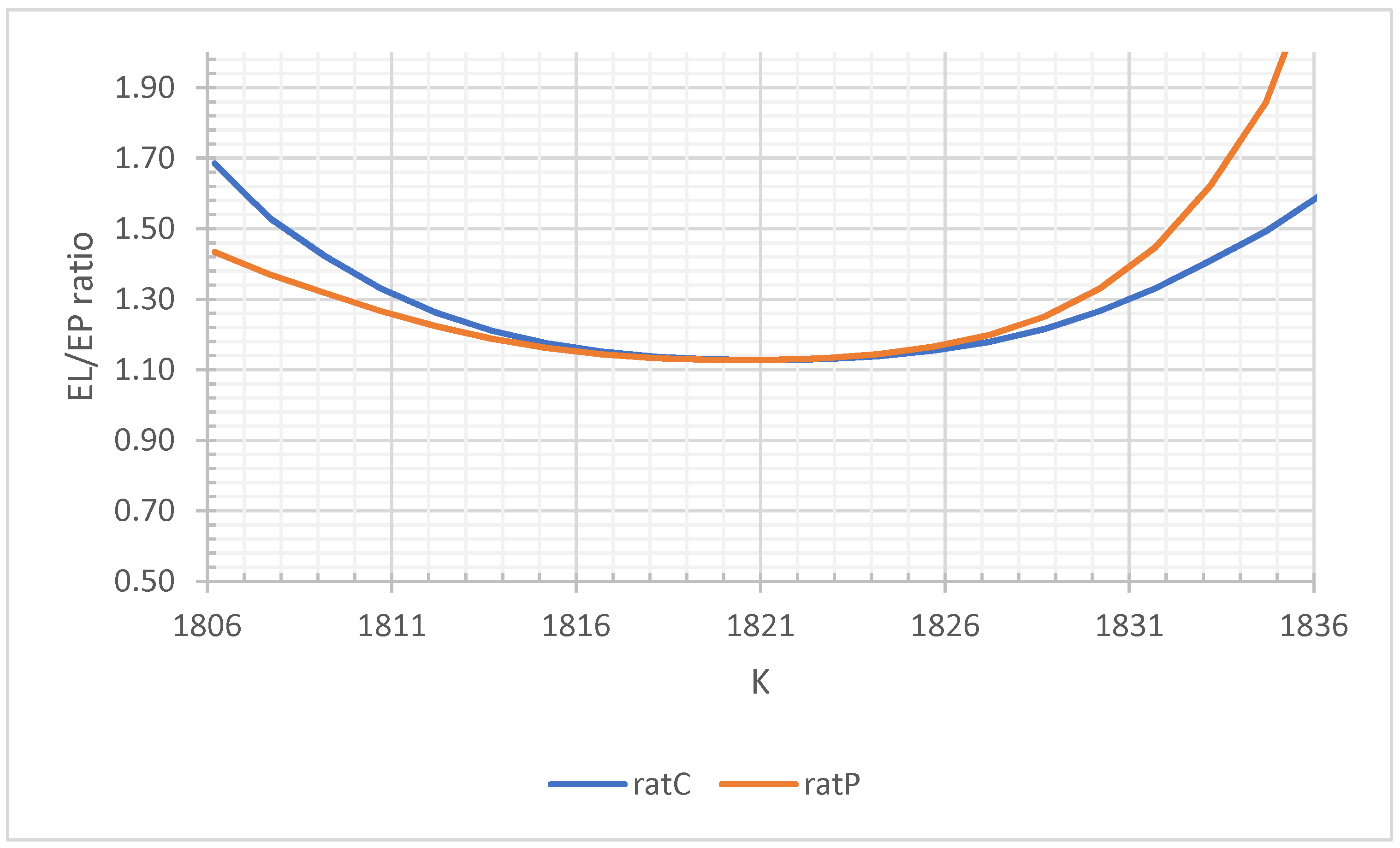Similarly, using (10) for the put binaries, columns 9 to 11 show the values of $\mathbb{E}{Y}^{+}$ and $\mathbb{E}{Y}^{-}$ and their EL/EP ratio (ratP) at each strike.

Next consider the prospective trade at strike 1821.20 with EP of 23.52. At the maximal risk tolerance level of $\lambda =1,$ the risk constraint says that we are looking for trades with EL below 23.52. Since EL is 26.52, the risk constraint does not hold here. Moreover, the corresponding EL/EP ratio is 1.1297 which is larger than 1. Thus, the call at strike 1821.20 would not be an attractive trade. Further, none of the other trades satisfy our risk constraint. Figure 2 shows graphs of the two EL/EP ratios, ratC and ratP, as functions of the strike price. The put binaries have somewhat lower ratios at the smaller strikes and the calls somewhat lower at the larger strikes. But both graphs stay above the level of 1 throughout their ranges, making all the trades on offer rather unattractive from an EPEL point of view. This effect may be due to trading cost being non-zero on the Nadex platform, which is inherent in the prices on offer and the use of the Nadex PITM-s.

Now the cardinal question is this: does the analysis so far imply that the EPEL trader should avoid dealing in the Nadex binary options? Not necessarily! The EPEL analysis above is based on the Nadex probability assessment of the price dynamics of the underlying asset. The trader may well have a different assessment, which may change the attractiveness to him of the trades on offer. We address this issue by first estimating a $GBM\left(\mu ,\sigma \right)$ model that describes the Nadex PITM assessment. Then we illustrate the effects of varying parameter choices in the model that may reflect the trader’s own assessment better.

For this purpose, denote the PITM at the $i$-th strike by $PIT{M}_i$. Recall that this is 100 times the probability of the event that $S_1>K_i$. Hence under the $GBM\left(\mu ,\sigma \right)$ model, we have the equation

$$PIT{M}_i=100\left(1-\Phi \left([\log (K_i/S_0)-\mu ]/\sigma \right)\right)=100\Phi \left((M_i+\mu \right)/\sigma )$$

(15)

Setting $z_i={\Phi }^{-1}(PIT{M}_i/100)$, (15) can be rewritten in the form

$$M_i=\sigma z_i-\mu$$

(16)

The pairs $\left(M_i,z_i\right)$ are given in the last two columns of Table 2, and Figure 3 plots them together with a fitted line with a very high $R^2$. The parameter estimates are $\mu$ = −0.0008 and $\sigma$ = 0.0051. This strongly suggests that a very good description of the Nadex PITM-s is provided by a GBM(−0.0008, 0.0051) model. The estimates $\mu$ = −0.0008 and $\sigma$ = 0.0051 may be called the implied drift and volatility parameters of the underlying asset.

However, with the Nadex PITM-s, it turned out above that the EPEL trader does not have attractive trades on offer. But the trader’s own assessment of the PITM-s may differ from that of Nadex. For example, the trader may have reason to think that the value of −0.0008 for the drift parameter does not express his positive (or negative) anticipation of the price movements of the underlying asset on the day ahead. If so, the trader can substitute his assessments of $\mu$ and $\sigma$ into (7) and (10) to calculate the corresponding values of EP, EL and the EL/EP ratios of the call and put trades. Then he can reconsider the attractiveness of the trades on offer.

The top left panel in Figure 3 shows how this pans out if the value of the drift parameter μ is increased by 0.0030 to 0.0022, while the volatility parameter $\sigma$ is left unchanged. The graph for the call binaries shows that there are strikes with EL/EP ratios below 0.5. For example, the call trade at strike 1821.2 now has EP = 0.3383. With risk tolerance at $\lambda =0.5$, the risk constraint requires an EL below 0.5 × 0.3383 = 0.1692. Since the EL here is 0.1557, this constraint holds and this would be an attractive trade. This will not be the case for a trader with lower risk tolerance. The smallest EL/EP ratio is 0.3305 at the first strike. Hence if the trader has risk tolerance below this number, none of the call trades will be attractive. Turning to the put binaries, their EL/EP ratios are all substantially higher than before, so that they are even less attractive under this scenario. These findings are intuitively reasonable under this scenario. If the underlying drift rate increases, the price of the underlying tends to increase over the day and the probability of the strike being exceeded at expiry also increases, making the call trades more attractive, but the put trades more unattractive.

The top right panel in Figure 4 shows that the opposite happens when the drift parameter μ is decreased to −0.0038, while the volatility parameter σ is left unchanged at σ = 0.0051. Now there are put binaries available with EL/EP ratio as low as 0.4014 while all the call binaries have ratios much above 1 and thus become less attractive. The two bottom panels show what happens if the drift parameter is unchanged at −0.0008 and the volatility parameter is either higher at 0.01 or lower at 0.0035. At μ = −0.0008 and σ = 0.01 the put binaries at the smaller strikes are more attractive while the calls at the larger strikes are more attractive; vice versa, when leaving the drift parameter unchanged at $\mu =-0.0008$ while decreasing the volatility to $\sigma =-0.0035$.

Hence to answer the cardinal question above: the trader should make his own assessment of the PITM-s for the day and then the EPEL approach provides helpful guidance on where to find attractive trades if he wishes to act on his assessment. This is due to EPEL taking both reward and risk tolerance into account. By contrast, the analysis of the Nadex data based on the BS formulas, appears lacking in these respects—possibly due to the notion of risk-neutrality playing a major role there.

5. Portfolios of Binary Options: Theory

As in all trading contexts, the trader in binaries is also faced with the matter of selecting among many possible choices: what strikes on offer to take up and what call or put binaries to buy. This issue may be phrased as a portfolio selection problem. In this section we develop the EPEL approach to dealing with this problem.

Assume that the trader operates with two budgets, representing the largest amounts that are planned to invest in the call and the put binaries respectively. An overall portfolio of binaries will result from a given allocation of these budgets to the different binary trades and this portfolio will also have a reward EP and a risk EL. We choose the portfolio allocation to maximize its EP subject to the same risk constraint as before, namely that its EL is no more than the risk tolerance fraction $\lambda$ of its EP.

Turning to the details of the portfolio EPEL approach, denote the trader’s budgets for the call and the put binaries by $B^C$ and $B^P$. Moreover, denote the number of strike levels by I so that there are I call and I put binaries corresponding to the strikes $\left\{K_i, i=1,\dots ,I\right\}$ on offer, at the prices $C_i$ and $P_i$ respectively. Suppose further that the trader invests the amount $B_i^C$ into the ith call and the amount $B_i^P$ into the $i$th put binary, where the allocation $\left\{B_I^C,\dots ,B_I^C ;B_I^P,\dots ,B_I^P\right\}$ is subject to the requirements

$${{\displaystyle \sum }}_{i=1}^I{B}_i^C\le B^C \mathrm{and} {{\displaystyle \sum }}_{i=1}^I{B}_i^P\le B^P.$$

(17)

The P&L on maturity discounted back to the present moment due to the $i$th call is $X_i$ given by (3) with $C$ and $K$ replaced by $C_i$ and $K_i$, respectively. The P&L on maturity discounted back to the present moment due to the $i$th put is $Y_i$ given by (9) with $P$ and $K$ replaced by $P_i$ and $K_i$, respectively. The amount $B_i^C$ invested into the $i$th call, will buy $n_i^C=B_i^C/C_i$ calls and result in a P&L of $n_i^C{X}_i=B_i^C{X}_i/C_i=B_i^C{R}_i^C$, where $R_i^C=X_i/C_i$ is the arithmetic return of the $i$th call. Similarly, the amount $B_i^P$ invested into the $i$th put, results in a P&L of $B_i^P{R}_i^P$, where $R_i^P=Y_i/P_i$ is the arithmetic return of the $i$th put. Then the P&L for this portfolio is

$$Z={{\displaystyle \sum }}_{i=1}^I\left(B_i^C{R}_i^C+B_i^p{R}_i^p\right).$$

(18)

From (3) modified for the present situation

$$R_i^C=D_i^C\mathbb{I}\left(S_1>K_i\right)-1 \mathrm{and} R_i^P=D_i^P\mathbb{I}\left(S_1\le K_i\right)-1$$

(19)

where $D_i^C=Q{e}^{-r}/C_i$ and $D_i^P=Q{e}^{-r}/P_i.$ Substituting into (18) gives

$$Z={{\displaystyle \sum }}_{i=1}^I\{B_i^C\left(D_i^C\mathbb{I}\left(S_1>K_i\right)-1\right)+B_i^p\left(D_i^p\mathbb{I}\left(S_1\le K_i\right)-1\right)\}.$$

(20)

The total portfolio EP and EL as functions of the allocation $\left\{B_1^C,\dots ,B_I^C;B_1^P,\dots ,B_I^P\right\}$ are given by $\mathbb{E}{Z}^{+}$ and $\mathbb{E}{Z}^{-}$ and the aim is to choose the allocation to

$$\mathrm{maximize} \mathbb{E}{Z}^{+} \mathrm{subject} \mathrm{to} \mathbb{E}{Z}^{-}\le \lambda \mathbb{E}{Z}^{+}$$

(21)

as well as (17) and other requirements mentioned below. This maximization problem can be formulated and solved by linear programming, as follows. Define $K_0=-\infty$, $K_{I+1}=+\infty$ and consider the events $K_j<S_1\le K_{j+1}$ for $j=0,1,\dots ,I.$ On $K_j<S_1\le K_{j+1}$ we have $S_1>K_i$ for $i=1,\dots ,j$ and also $S_1\le K_i$ for $i=j+1,\dots ,I+1$. Thus

$$Z={{\displaystyle \sum }}_{i=1}^j{B}_i^C{D}_i^C+{{\displaystyle \sum }}_{i=j+1}^I{B}_i^P{D}_i^P-{{\displaystyle \sum }}_{i=1}^I(B_i^C+B_i^P) \mathrm{if} K_j<S_1\le K_{j+1}$$

(22)

Introduce new variables

$$V_j={{\displaystyle \sum }}_{i=1}^j{B}_i^C{D}_i^C+{{\displaystyle \sum }}_{i=j+1}^I{B}_i^P{D}_i^P-{{\displaystyle \sum }}_{i=1}^I(B_i^C+B_i^P), j=0,1,\dots ,I$$

(23)

so that

$$Z={{\displaystyle \sum }}_{j=0}^I{V}_j\mathbb{I}(K_j<S_1\le K_{j+1}).$$

(24)

This states that $Z$ has a discrete distribution with mass points the $V_j$-s. Denote the positive and negative parts of $V_j$ by $V_j^{+}$ and $V_j^{-}$. Then (24) yields

$$Z^{+}={{\displaystyle \sum }}_{j=0}^I{V}_j^{+}\mathbb{I}(K_j<S_1\le K_{j+1}) \mathrm{and} Z^{-}={{\displaystyle \sum }}_{j=0}^I{V}_j^{-}\mathbb{I}(K_j<S_1\le K_{j+1}).$$

(25)

Under the $GBM\left(\mu ,\sigma \right)$ model

$$\mathbb{P}\left(K_j<S_T\le K_{j+1}\right)=\Phi \left(a_j\right)-\Phi \left(a_{j+1}\right)={\mathbb{P}}_j$$

(26)

with $a_j$ as in (6) with $K$ replaced by $K_j$. Hence the portfolio EP and EL are given by

$$\mathbb{E}{Z}^{+}={{\displaystyle \sum }}_{j=0}^I{\mathbb{P}}_j{V}_j^{+} \mathrm{and} \mathbb{E}{Z}^{+}={{\displaystyle \sum }}_{j=0}^I{\mathbb{P}}_j{V}_j^{-}$$

(27)

respectively. Our objective is to choose the allocation $\left\{B_I^C,\dots ,B_I^C;B_I^P,\dots ,B_I^P\right\}$ to

$$\mathrm{Maximize} {{\displaystyle \sum }}_{j=0}^I{\mathbb{P}}_j{V}_j^{+} \mathrm{subject} \mathrm{to} {{\displaystyle \sum }}_{j=0}^I{\mathbb{P}}_j{V}_j^{-}\le \lambda {{\displaystyle \sum }}_{j=0}^I{\mathbb{P}}_j{V}_j^{-}$$

(28)

and (17). We have two sets of the variables, namely $\left\{B_I^C,\dots ,B_I^C;B_I^P,\dots ,B_I^P\right\}$ and $\left\{V_0^{+},\dots ,V_I^{+};V_0^{-},\dots ,V_I^{-}\right\}$. They are related by (23) which may be written as the linear equations

$$V_j^{+}-V_j^{-}-{{\displaystyle \sum }}_{i=1}^j{B}_i^C{D}_i^C-{{\displaystyle \sum }}_{i=j+1}^I{B}_i^P{D}_i^P+{{\displaystyle \sum }}_{i=1}^I(B_i^C+B_i^P)= 0, j=0,1,\dots ,I$$

(29)

Further constraints may be added to force diversification. Two possibilities are

$$B_i^C\le f^C{B}^C \mathrm{and} B_i^P\le f^P{B}^P, i=1,\dots ,I$$

(30)

where $f^C$ and $f^P$ are fractions chosen to limit the parts of the total budgets that may be invested into any single call or put binary. The objective function (28) and all the constraints (17), (29), and (30) are linear in the relevant variables, so that the problem of finding the maximized allocation can be solved by standard LP solvers.

It may not be practical to allow small amounts allocated to many different binaries. To prevent this from happening we can add the constraints

$$g^C{B}^C{L}_i^C\le B_i^C\le f^C{B}^C{L}_i^C \mathrm{and} g^P{B}^P{L}_i^P\le B_i^P\le f^P{B}^P{L}_i^P, i=1,\dots ,I$$

(31)

where $g^C$ and $g^P$ are lower bounds, above which the fractions of the amounts to be invested in an option must be if they are not zero. The $L_i^C-s$ and $L_i^P-s$ are {0,1} variables, taking the value 0 if nothing is to be invested in option $i$ and 1 if at least the amounts $g^C{B}^C$ or $g^P{B}^P$ are to be invested, respectively. The constraints (31) turn the problem into a mixed integer LP (MILP) problem, for which standard solvers are also available. We used MILPSOLVE of SAS IML in the results reported in this paper.

The trader may also be interested in the sub-metrics that make up the EP and EL values, namely the probability of a positive (negative) outcome of the portfolio P&L and the expected profit (loss) conditionally given a positive (negative) P&L. These are given by

$$\begin{gathered} \mathrm{ProbP}=\mathbb{P}\left(Z>0\right)={{\displaystyle \sum }}_{j=0}^I\mathbb{I}(V_j>0){\mathbb{P}}_j \mathrm{and} \mathrm{EPGP}=\mathbb{E}[Z^{+}|Z>0]=\mathbb{E}{Z}^{+}/\mathbb{P}\left(Z>0\right) \\ \mathrm{ProbL}=\mathbb{P}\left(Z<0\right)={{\displaystyle \sum }}_{j=0}^I\mathbb{I}(V_j<0){\mathbb{P}}_j \mathrm{and} \mathrm{ELGL}=\mathbb{E}[Z^{-}|Z<0]=\mathbb{E}{Z}^{-}/\mathbb{P}\left(Z<0\right) \end{gathered}$$

(32)

Note that since $Z$ is discretely distributed, it may happen that $Z=0$ with positive probability, which is given by $\mathrm{Prob}0=\mathbb{P}\left(Z=0\right)={{\displaystyle \sum }}_{j=0}^I\mathbb{I}\left(V_j=0\right){\mathbb{P}}_j$.

Extensive practical illustrations of the results above are given in the next section.

6. EPEL Portfolios of Binaries: Illustration

In this section we illustrate the optimal binary option portfolio allocation theory of the previous section. The Nadex data are used again. Four scenarios are discussed, namely the trader anticipates positive drift (Case 1), negative drift (Case 2), higher volatility (Case 3), and lower volatility (Case 4). In all cases the total call and put budgets are both taken as 100 units, so that the allocations can be interpreted as percentages of the total budgets. For each case, we consider two specifications for the risk tolerance parameter, namely $\lambda =0.3$ (low risk tolerance) and $\lambda =0.9$ (mild risk tolerance). Moreover, two choices of the diversification parameters are treated, namely $f^C=f^P=1$ and $f^C=f^P=1/5$. The first choice allows 100% of the budget at any single strike (no diversification). The second choice allows no more than 20% of the budget at any single strike (substantial diversification).

Cases 1 and 2. To model the positive drift scenario of Case 1, the drift rate is taken as $\mu =0.0022$ while the volatility is kept unchanged at $\sigma =0.0051$. This corresponds to the top left panel in Figure 4. The left block of

Table 3. EPEL binary portfolio allocations and features for Case 1 (left block) and Case 2 (right block). In Case 1 $\mu =0.0022$ and in Case 2 $\mu =-0.0038$. In both cases $\sigma =0.0051$ and $S_0=1822$. Results based on Nadex gold binary data of 8 February 2022.

		EPEL Allocation Results for Case 1						EPEL Allocation Results for Case 2
			1-1	1-2	1-3	1-4			2-1	2-2	2-3	2-4
		$\mathit{\lambda }$	0.3	0.3	0.9	0.9		$\mathit{\lambda }$	0.3	0.3	0.9	0.9
		fC	1	0.2	1	0.2		fP	1	0.2	1	0.2
		EP	95.3	88.7	173.7	154.3		EP	92.0	88.1	160.7	142.4
		EL	28.6	26.6	72.9	61.5		EL	27.6	26.4	68.3	57.0
		EL/EP	0.300	0.300	0.420	0.399		EL/EP	0.300	0.300	0.425	0.400
		ProbP	0.271	0.327	0.271	0.327		ProbP	0.317	0.377	0.317	0.377
		ProbL	0.423	0.423	0.729	0.673		ProbL	0.369	0.369	0.683	0.623
		Prob0	0.306	0.251	0.000	0.000		Prob0	0.314	0.254	0.000	0.000
		EPGP	351.5	271.6	640.7	472.2		EPGP	289.8	233.5	506.1	377.4
		ELGL	67.6	63.0	100.0	91.3		ELGL	74.9	71.7	100.0	91.6
K	C	PITM	BC1	BC2	BC3	BC4	P	PITM	BP1	BP2	BP3	BP4
1806.2	95.25	97.15	0	0	0	0	10.75	11.55	0	0	0	0
1807.7	93.75	95.92	0	0	0	0	12.25	15.03	0	0	0	20
1809.2	92.00	94.28	0	0	0	0	14.00	19.15	0	6	0	20
1810.7	89.50	92.16	0	0	0	0	16.50	23.88	48	20	100	20
1812.2	86.25	89.50	0	0	0	0	19.75	29.20	0	20	0	20
1813.7	82.00	86.24	0	0	0	0	24.00	34.99	0	0	0	20
1815.2	76.75	82.36	0	0	0	0	29.25	41.16	0	0	0	0
1816.7	70.75	77.85	0	0	0	0	35.25	47.55	0	0	0	0
1818.2	64.00	72.76	0	14	0	0	42.00	54.00	8	11	0	0
1819.7	56.50	67.14	44	20	0	0	49.50	60.34	0	0	0	0
1821.2	51.50	61.11	0	20	0	0	54.50	66.41	44	20	0	0
1822.7	45.25	54.81	0	0	0	0	60.75	72.08	0	20	0	0
1824.2	38.00	48.38	8	2	0	0	68.00	77.23	0	3	0	0
1825.7	31.25	42.01	0	0	0	0	74.75	81.80	0	0	0	0
1827.2	25.50	35.84	0	0	0	0	80.50	85.74	0	0	0	0
1828.7	20.50	30.03	0	0	0	20	85.50	89.06	0	0	0	0
1830.2	16.50	24.69	0	20	0	20	89.50	91.78	0	0	0	0
1831.7	13.50	19.90	47	20	100	20	92.50	93.95	0	0	0	0
1833.2	11.25	15.73	0	5	0	20	94.75	95.65	0	0	0	0
1834.7	9.75	12.18	0	0	0	20	96.25	96.94	0	0	0	0
1836.2	8.50	9.24	0	0	0	0	97.50	97.89	0	0	0	0

reports results for this case. In line with the top left panel of Figure 4, showing that the put binaries are all unattractive, the optimal portfolios for Case 1 made no allocations to put binaries in all the sub-cases reported in the left block. The right block of Table 3 reports results for the negative drift scenario of Case 2. In line with the top right panel of Figure 4, showing that the call binaries are all unattractive, the optimal portfolios for Case 2 made no allocations to call binaries in all the sub-cases reported in the right block. Lines 2 to 4 show the numbers of the sub-cases and the values of the parameters in each sub-case. Lines 18 to 39 show the strikes in the first column while the binary call and put prices are shown in the columns C and P. The trader’s own PITM-s under the scenarios of Case 1 and Case 2 are shown in the two columns headed PITM. The optimal budget allocations for the four sub-cases of Case 1 (Case 2) are shown in the columns headed BC1–BC4 (BP1–BP4) in the two blocks. Rows 5 to 12 show the values of the EPEL features due to the optimal portfolio allocations for each of the sub-cases of Cases 1 and 2.

In sub-case 1-1 the trader has low risk tolerance with $\lambda =0.3$ but do not force diversification with the choice $f^C=1$. Here the EPEL method allocates 44% of the budget to the call at the strike 1819.7 and 47% to the call at 1831.7 and makes a small allocation of 8% to the call at strike 1824.2. The calls at the smaller strikes in the table may be described as offering “expensive but safe” trades, since their prices are high while their PITM-s are also high. By contrast the calls at larger strikes in the table may be described as offering “cheap but unsafe” trades, since their prices are low, but their PITM-s are also low. In between these extremes we have midrange trades. The trader of sub-case 1-1 anticipates price drift which would suggest going for the cheaper but unsafe trades, but his low risk tolerance suggests this need to be balanced by some safer lower risk trades. Option price also plays a role and doing the balancing with midrange trades, makes intuitive sense in these circumstances. The optimal EPEL allocation delivers a portfolio with an EP of 95.3 and EL of 28.6, having a ratio of 0.3 as specified with the choice of $\lambda$. The probabilities of making a profit or a loss are 0.271 and 0.423 respectively, while the probability of zero P&L is 0.306. Hence about 31% of trades done according to this allocation result in neither profit nor loss, while 27% yield a profit and 42% yield a loss. Thus, the ratio of loss to profit frequencies is 0.423/0.271 = 1.56. The average size of a profit, when there is a profit, is 351.5 and the average size of a loss, when there is a loss, is 67.6 so that the loss to profit size ratio is 67.6/351.5 = 0.19. Hence this allocation will lead to more frequent losses than profits, but the loss sizes will be much smaller than the profit sizes. These sub-metrics are somewhat contrary to each other, but the size ratio dominates the frequency ratio to the extent that their combination in the EL/EP ratio amounts to 0.3, yielding one overall metric in terms of which this would be a portfolio of good quality.

Sub-case 1-2 keeps the same low risk tolerance but requires more diversification with the choice $f^C=0.2$ so that no more than one-fifth of the budget may be placed at one strike. The EPEL allocation now spreads out over five strikes, with larger allocations and two strikes with smaller ones, all located close to the previous no-diversification strikes. The resulting EP and EL values are both slightly smaller and the EL/EP ratio still satisfies the 0.3 bound. The other EPEL features are changed somewhat, but the overall result may still be described as more frequent losses than profits, but much lower sized losses than profits.

Sub-case 1-3 relaxes the risk tolerance to $\lambda =0.9$ and reverts to the no-diversification parameter choice of sub-case 1-1. With risk tolerance so mild, the optimal EPEL portfolio now allocates the full budget to the strike at 1831.7. This is a cheap but unsafe trade and a reflection of the mild risk tolerance (or aggressive trading), coupled with the assumed price drift scenario which is anticipated to ameliorate the “unsafe” aspect of this allocation. The EL/EP ratio is only 0.42 and is therefore not binding at the optimal constraint value of 0.9. Trading with this portfolio can still be described as more frequent losses than profits, but with profit sizes being more than six times higher than loss sizes. Sub-case 1-4 brings the 20% diversification constraint back and this simply leads to the budget being spread out over five strikes centered around 1831.7. There is some improvement in the EL/EP ratio, but the same description still applies.

The right block of Table 3 reports the results of the optimal put portfolios in the same manner as left block. In many respects, this case represents the reverse of Case 1. The “expensive but safe” trades are now at the larger strikes toward the bottom of the table and the “cheap but unsafe” trades are towards the top of the table. The portfolio allocations can now be interpreted and understood with this in mind. At the low risk tolerance choice, the optimal allocations balance cheap but unsafe trades with midrange trades. At mild risk tolerance the optimal allocations concentrate on the cheap but unsafe trades, assuming that the anticipated underlying price decrease will save the day. For each fixed choice of the risk tolerance parameter, stricter diversification splits up the allocations to more strikes, but typically close to the prior ones.

Case 3. Here the trader anticipates no change in the drift rate but higher volatility and this is modelled by taking $\mu =-0.0008$ and $\sigma =0.01$. At the time of writing, the current volatility value of 0.0051 is rather low from a historical perspective and doubling it to 0.01 seems reasonable in terms of what a “higher volatility” specification would imply. This corresponds to the bottom left panel of Figure 4, which shows that the call binaries at the larger strikes are more attractive and the puts at the smaller strikes are more attractive. Hence the optimal portfolio may be expected to make both call and put allocations.

Table 4. Binary EPEL portfolio allocations and features for Case 3 with $\mu =-0.0008,$ $\sigma =0.01$ and $S_0=1822$ in the GBM models and with varying $\gamma$ and $f^C, f^C$ applied to the Nadex gold binary data of 8 February 2022.

				Case	3-1		3-2		3-3		3-4
				$\mathit{\lambda }$	0.3		0.3		0.9		0.9
				$\mathit{f}\mathit{C};\mathit{f}\mathit{P}$	1		0.2		1		0.2
				EP	317.33		276.87		347.92		276.87
				EL	95.20		80.79		117.92		80.79
				EL/EP	0.300		0.292		0.339		0.292
				ProbP	0.410		0.564		0.410		0.564
				ProbL	0.490		0.436		0.590		0.436
				Prob0	0.100		0.000		0.000		0.000
				EPGP	773.25		490.49		847.78		490.49
				ELGL	194.36		185.49		200.00		185.49
K	C	P	PITMC	PITMP	BC1	BP1	BC2	BP2	BC3	BP3	BC4	BP4
1806.2	95.25	10.75	78.55	21.45	0	70	0	20	0	100	0	20
1807.7	93.75	12.25	76.05	23.95	0	0	0	20	0	0	0	20
1809.2	92.00	14.00	73.40	26.60	0	14	0	20	0	0	0	20
1810.7	89.50	16.50	70.61	29.39	0	16	0	20	0	0	0	20
1812.2	86.25	19.75	67.70	32.30	0	0	0	20	0	0	0	20
1813.7	82.00	24.00	64.68	35.32	0	0	0	0	0	0	0	0
1815.2	76.75	29.25	61.56	38.44	0	0	0	0	0	0	0	0
1816.7	70.75	35.25	58.37	41.63	0	0	0	0	0	0	0	0
1818.2	64.00	42.00	55.12	44.88	0	0	0	0	0	0	0	0
1819.7	56.50	49.50	51.85	48.15	0	0	0	0	0	0	0	0
1821.2	51.50	54.50	48.56	51.44	0	0	0	0	0	0	0	0
1822.7	45.25	60.75	45.29	54.71	0	0	0	0	0	0	0	0
1824.2	38.00	68.00	42.05	57.95	0	0	0	0	0	0	0	0
1825.7	31.25	74.75	38.86	61.14	0	0	0	0	0	0	0	0
1827.2	25.50	80.50	35.76	64.24	0	0	0	0	0	0	0	0
1828.7	20.50	85.50	32.74	67.26	0	0	0	0	0	0	0	0
1830.2	16.50	89.50	29.84	70.16	0	0	20	0	0	0	20	0
1831.7	13.50	92.50	27.06	72.94	0	0	20	0	0	0	20	0
1833.2	11.25	94.75	24.42	75.58	23	0	20	0	0	0	20	0
1834.7	9.75	96.25	21.93	78.07	0	0	20	0	0	0	20	0
1836.2	8.50	97.50	19.59	80.41	77	0	20	0	100	0	20	0

reports some results. The layout of the table is slightly different from the Table 3 since more columns are needed to show both call and put prices as well as PITM-S and allocations. In keeping with the bottom left panel of Figure 4, the optimal EPEL call allocations are to the larger strikes (the cheap but unsafe call trades) and the put allocations to the smaller strikes (the cheap but unsafe put trades) in all sub-cases. The only difference between the cases is the extent of the concentration of the allocations to the extremes due to different diversification parameter choices. These allocations seem intuitively reasonable, since higher volatility implies higher likelihood of extreme movements of the price of the underlying, which in turn may lead to the price moving from its initial level in the middle of the table at the start of the day, to the extreme ends of the table and thus getting higher profits. A notable difference with Cases 1 and 2 is that the profit frequencies are now better balanced, while profit sizes are much larger than the loss sizes. So, trading results here would be characterized by well-balanced frequencies of trade events, but having relatively smaller size loss events than profit events. These results suggest that favorable EPEL trading is possible in this high volatility environment.

Case 4. Here the trader anticipates no change in the drift rate but lower volatility and this is modelled by taking $\mu =-0.0008$ and $\sigma =0.0035$. As noted above, the current volatility value of 0.0051 is already on the low side and lowering it to 0.0035 moves it into a very low volatility scenario. This corresponds to the bottom right panel of Figure 4 which shows that the call binaries at the smaller strikes are more attractive and the puts at the larger strikes are more attractive.

Table 5. Binary EPEL portfolio allocations and features for Case 4 with $\mu =-0.0008,$ $\sigma =0.0035$ and $S_0=1822$ in the GBM models and with varying $\gamma$ and $f^C, f^P$ applied to the Nadex gold binary data of 8 February 2022.

				Case	4-1		4-2		4-3		4-4
				$\mathit{\lambda }$	0.3		0.3		0.9		0.9
				$\mathit{f}\mathit{C};\mathit{f}\mathit{P}$	1		0.2		1		0.2
				EP	10.32		5.42		30.40		24.36
				EL	3.10		1.63		19.66		14.31
				EL/EP	0.30		0.30		0.65		0.59
				ProbP	0.58		0.52		0.76		0.70
				ProbL	0.03		0.05		0.24		0.30
				Prob0	0.39		0.44		0.00		0.00
				EPGP	17.92		10.49		40.17		35.01
				ELGL	88.49		35.78		80.83		47.04
K	C	P	PITMC	PITMP	BC1	BP1	BC2	BP2	BC3	BP3	BC4	BP4
1806.2	95.25	10.75	98.81	1.19	9	0	20	0	0	0	0	0
1807.7	93.75	12.25	97.84	2.16	76	0	20	0	0	0	20	0
1809.2	92.00	14.00	96.29	3.71	0	0	0	0	0	0	20	0
1810.7	89.50	16.50	93.93	6.07	0	0	0	0	0	0	20	0
1812.2	86.25	19.75	90.53	9.47	0	0	0	0	100	0	20	0
1813.7	82.00	24.00	85.90	14.10	15	0	0	0	0	0	20	0
1815.2	76.75	29.25	79.95	20.05	0	0	8	0	0	0	0	0
1816.7	70.75	35.25	72.70	27.30	0	0	0	0	0	0	0	0
1818.2	64.00	42.00	64.35	35.65	0	0	0	0	0	0	0	0
1819.7	56.50	49.50	55.26	44.74	0	0	0	0	0	0	0	0
1821.2	51.50	54.50	45.89	54.11	0	0	0	0	0	0	0	0
1822.7	45.25	60.75	36.76	63.24	0	0	0	0	0	0	0	0
1824.2	38.00	68.00	28.32	71.68	0	12	0	7	0	0	0	20
1825.7	31.25	74.75	20.95	79.05	0	0	0	0	0	0	0	20
1827.2	25.50	80.50	14.85	85.15	0	0	0	0	0	100	0	20
1828.7	20.50	85.50	10.07	89.93	0	0	0	0	0	0	0	20
1830.2	16.50	89.50	6.53	93.47	0	0	0	0	0	0	0	20
1831.7	13.50	92.50	4.04	95.96	0	0	0	0	0	0	0	0
1833.2	11.25	94.75	0.28	99.72	0	0	0	19	0	0	0	0
1834.7	9.75	96.25	0.10	99.90	0	88	0	20	0	0	0	0
1836.2	8.50	97.50	0.03	99.97	0	0	0	20	0	0	0	0

reports some results for the EPEL allocation in the same form as Table 4 and with the same specifications of the risk tolerance and diversity parameters. These allocations are in line with the suggestions from Figure 4. However, the EPEL features for this low volatility case differ much from those of the high volatility Case 3. For example, the frequencies of profits are now larger than those of losses, whereas it was the other way round in Case 3. The profit sizes are lower than the loss sizes, whereas they were much larger in Case 3. Hence results of trading in a low volatility scenario is potentially much different from trading in a high volatility scenario, but still with good performance since the risk specifications are still satisfied. It notable is that the EP and EL values are all much smaller here than in Case 3. This implies that the budgets used can be increased substantially when trading in this low volatility scenario—which would be quite natural.

To summarize the illustration, if the trader is correct in anticipating the direction of drift and changes in volatility of the price of the underlying, and if the specification of the parameters $\mu$ and $\sigma$ are cogent, then the trader can get good quantitative guidance from the EPEL methodology on how to pitch his portfolio. The specifications can be varied to check on the stability of the allocations before final decisions are made for the day or other period to maturity. The type of analysis reported above, can also be repeated on a regular intra-period basis. At present these possibilities are open research items.

7. Conclusions

The EPEL approach supplies the trader with suitable reward and risk metrics in terms of which to judge the quality of trades. This paper applies this approach to trading in binary options. The formulas for the EP and the EL of call and put binary options are derived and illustrated with practical data from the Nadex platform. The illustration leads to identifying the GBM with implied drift and volatility as a suitable model to describe the price process of the underlying asset. The trader can vary these parameters to suit his anticipation of price movement of the underlying asset, thereby finding attractive trades with the EPEL formulas. This is contrasted with the use of the BS formulas—which is found lacking in effectiveness in this illustration. The matter of selecting good combinations of trades at different strikes on the option ladder, is formulated and shown to amount to linear programming problems. This enables efficient solutions, taking risk tolerance as well as diversification requirements into account. This is also illustrated with the Nadex data under various price drift trend and volatility scenarios.

Several further issues remain to be investigated in future work, following the EPEL approach applied to binary trading. Here is a partial list.

(1)

While the paper focused mostly on one day binary trades, the application of EPEL ideas to shorter or longer period trades, also needs more attention.

(2)

Deciding what the best risk tolerance level is at which to trade consistently profitable, is an open question. A related issue is that of using a risk tolerance level that changes with market volatility over time. During high volatility markets, the risk tolerance level should be lower than during low volatility markets.

(3)

Modeling the price process of the underlying asset by the GBM, may not be adequate for some assets. For instance, it cannot cater for features of real price processes such as non-constant volatility, fat-tailed distributions, price jumps, etc. To enable reliable estimation and prediction of the required EPEL probabilities, more flexible stochastic processes should be used. Some suitable examples are in the references Stojkoski et al. (2020) or Fu and Hirsa (2021). Both papers apply more general underlying price models to option pricing, finding extended equivalents of the BS formulas in the risk-neutral type context. However, using such generalized models with the EPEL approach have not been explored yet, but are outside the (introductory) scope of this paper.

(4)

In addition to the previous point, modelling the price process could incorporate technical analysis features and economic factors as well as sentiment analysis and the other important factors listed in Cofnas (2016). The Nadex platform and many other trading platforms, provide the trader with technical analysis tools to help in this regard. Some studies have been published on the possible success obtainable in this way; see e.g., Rumpa et al. (2021) or Kolkova and Lenertova (2016). The results of such back-testing studies can at best be described as mixed. Still, analogous studies involving the EPEL approach should be done, but are also outside the scope of this paper.

(5)

The notion of implied volatility based on the BS formula and the notions of implied drift and volatility discussed in Section 4, are instances of jointly analyzing underlying spot prices and option prices simultaneously. This is a developing topic which may lead to deeper understanding of price processes in equity markets. A striking statement in Begin et al. (2020) reads “We exploit the richness of stock option data to extract the expected risk premium associated with each risk factor, thereby avoiding the exclusive use of noisy realizations of historical equity returns”. Can the EPEL approach contribute in this regard?

(6)

The Nadex binaries are actually American type options since the holder can close them at any time and need not wait for expiry. This feature was not considered in this paper and the development of an EPEL version applicable to trading American binary options, is an open issue at present. A relevant reference is Gao (2017) who deals with early exercise of British binaries, but follows the no-arbitrage approach. Further literature that may be useful to develop the EPEL approach for American options, are Aretz et al. (2018) and Chiang et al. (2018). These papers also follow the risk-neutral approach.

Answering these questions will require extensive back-testing studies. Parts of this research are on-going, but not yet at the stage where we have definitive results to report.