

Evaluating Feature Selection Methods for Accurate Diagnosis of Diabetic Kidney Disease
 ,
,  , , , , ,
  and
and
Abstract
1. Introduction
Related Work
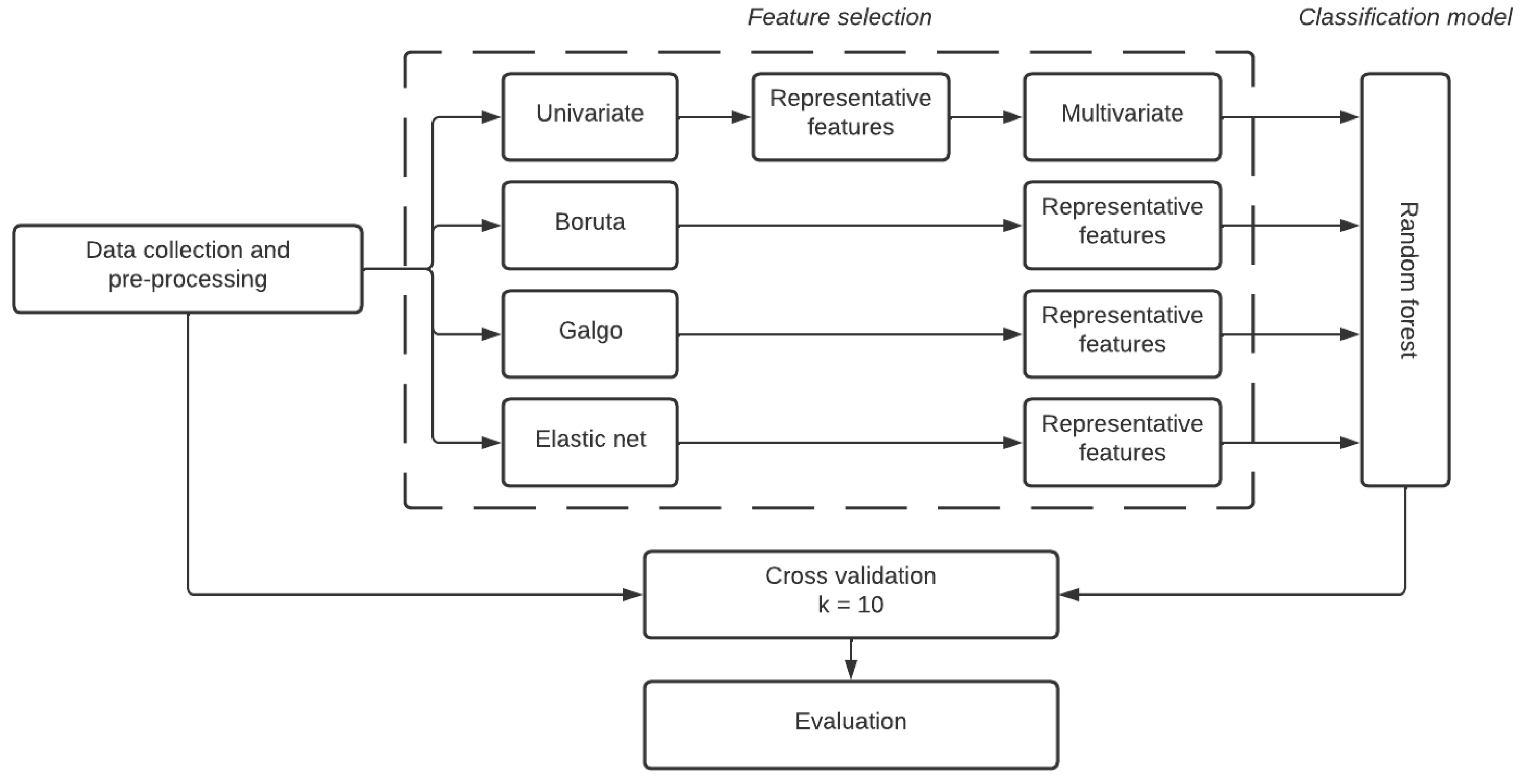
2. Materials and Methods
2.1. Dataset Description
- Inclusion criteria for cases:
- -
- Patients diagnosed with T2D according to the ADA criteria: fasting glucose equal to or greater than 126 mg/dL;
- -
- Any gender;
- -
- Affiliated beneficiaries to the IMSS with active and up-to-date benefits at time of enrollment;
- -
- Not having any family members participating in the study;
- -
- Patients who agreed to participate in the study and signed the informed consent form;
- -
- Adults diagnosed before the age of 55, with the current age for inclusion being between 35 and 85 years.
- Inclusion criteria for controls:
- -
- Individuals aged between 35 and 85 years, without meeting the criteria for metabolic syndrome (according to the International Adult Treatment Panel (ATP) III criteria);
- -
- Any gender;
- -
- Not having any family members participating in the study;
- -
- Individuals who agreed to participate in the study and signed the informed consent form;
- -
- Fasting glucose (12 h) below 100 mg/dL, and post-load glucose levels below 140 mg/dL two hours after ingesting 75 g of glucose.
- Exclusion criteria:
- -
- Beneficiaries with temporary or seasonal insurance coverage
- -
- Individuals without a permanent residence of those who cannot be reached by phone, either at their home or through a family member;
- -
- Woman in the climacteric stage.
2.1.1. Clinical Variables
2.1.2. Data Pre-Processing
2.2. Feature Selection Methodologies
2.2.1. Boruta
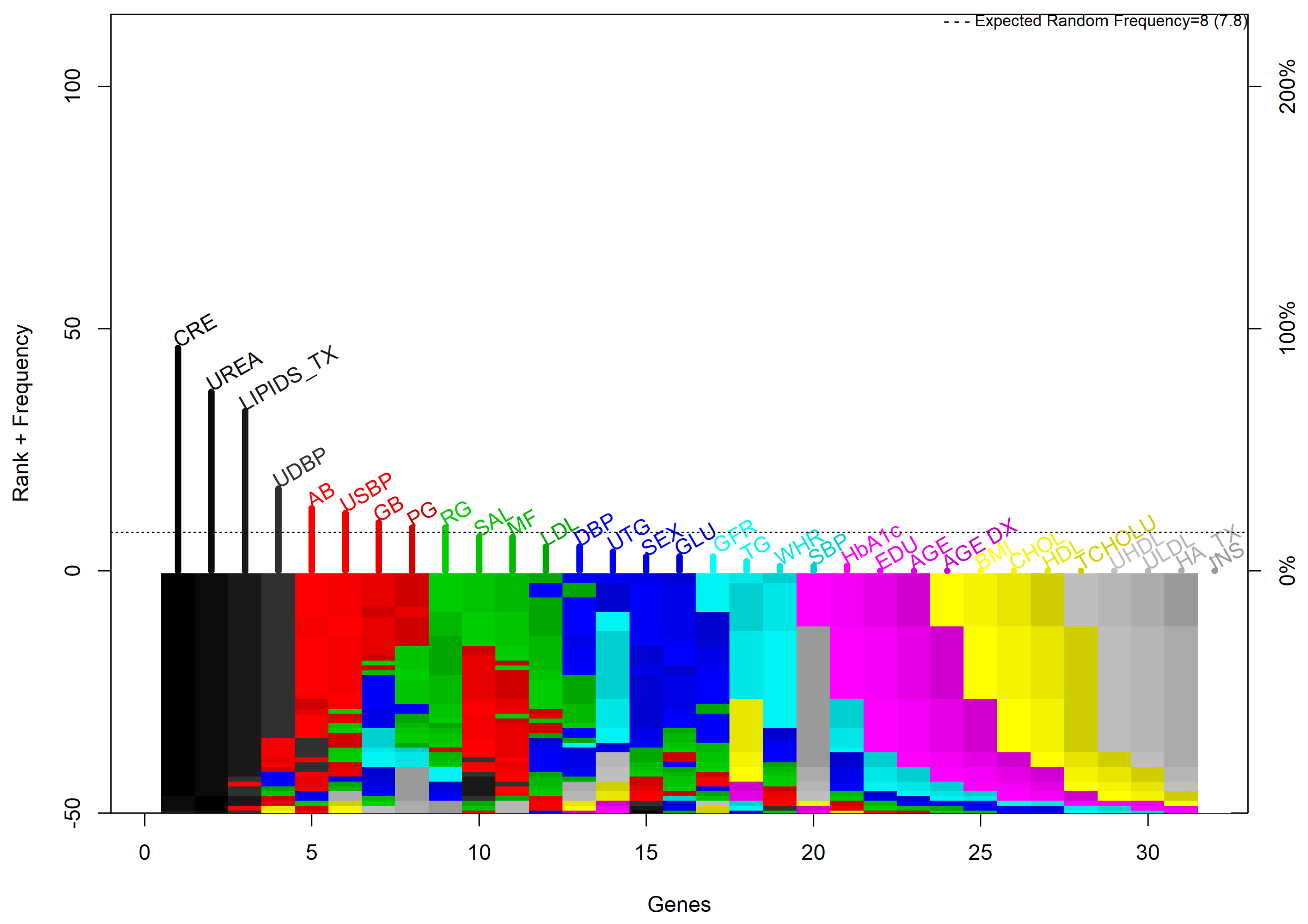
2.2.2. GALGO
- Setting up the analysis. The input and the outcome features are specified, as well as the parameters that define the GA environment (gene expression), the classification method, and the error estimation.
- Searching for relevant multivariate models. Starting from a random population of chromosomes, the GA method can find a diverse collection of good local solutions.
- Refinement and analysis of the population of selected chromosomes. The chromosomes selected from the GA are subjected to a backward selection strategy, aiming to obtain a model with a chromosome population that significantly contributes to the classification accuracy.
- Development of a representative statistical model. A single representative model is obtained; for this stage, a forward selection strategy was implemented based on the step-wise inclusion of the most prevalent genes in the chromosome population.
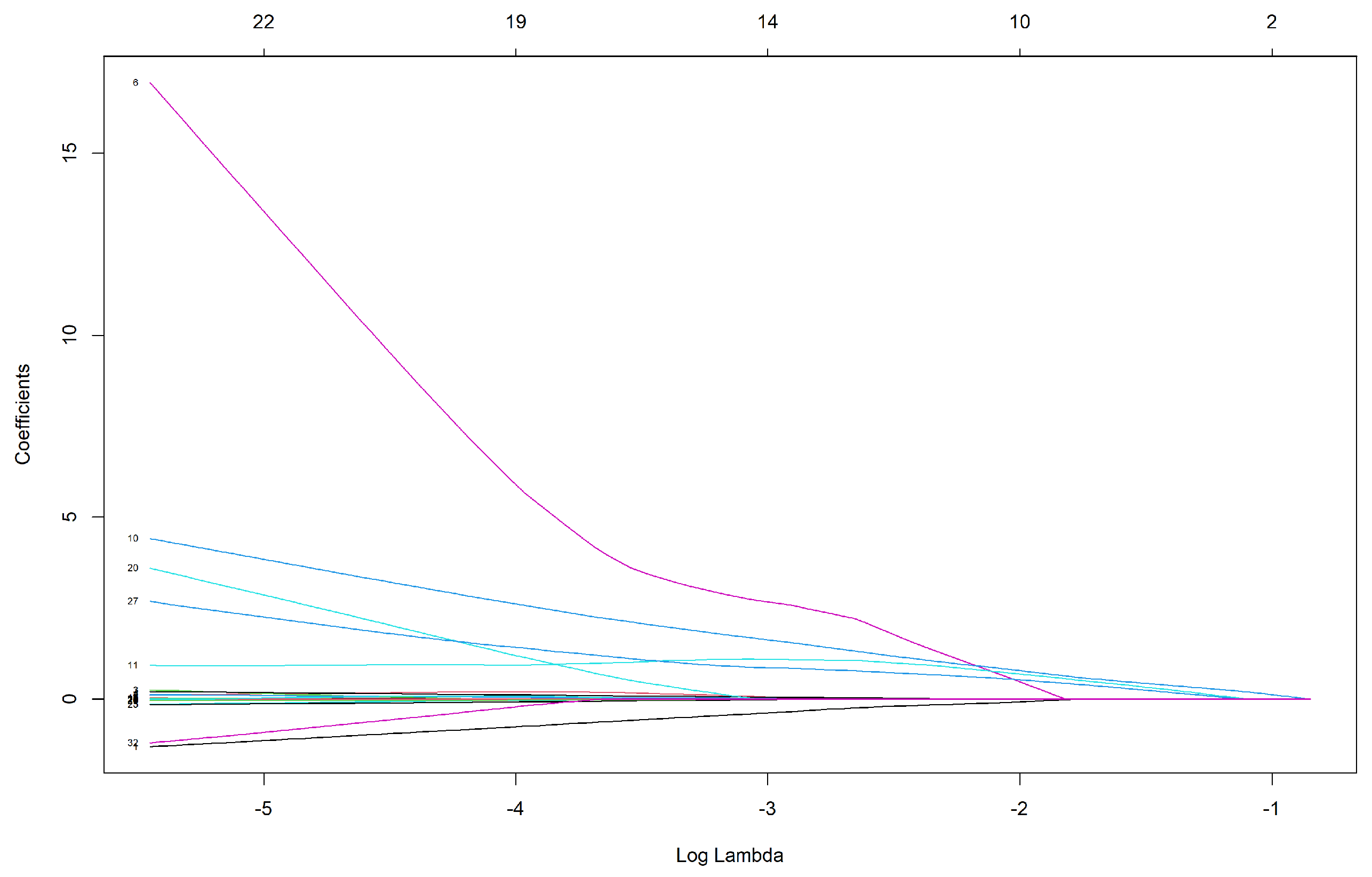
2.2.3. Elastic Net
- , LASSO, a penalized least squares method imposing an penalty on the regression coefficients, does a continuous shrinkage and automatic variable selection.
- , minimizes the residual sum of squares subject to a bound of the -norm of the coefficients. Ridge regression achieves its better prediction performance through a bias-variance trade-off; however, this method cannot produce a parsimonious model due to it always keeping all the predictors.
2.3. Classification Method
Random Forest
2.4. Evaluation Metrics
2.5. Cross Validation
2.6. Interpretability
3. Results
3.1. Comparison to Established Feature Selection Methods
3.1.1. Univariate and Multivariate Feature Selection
3.1.2. Boruta
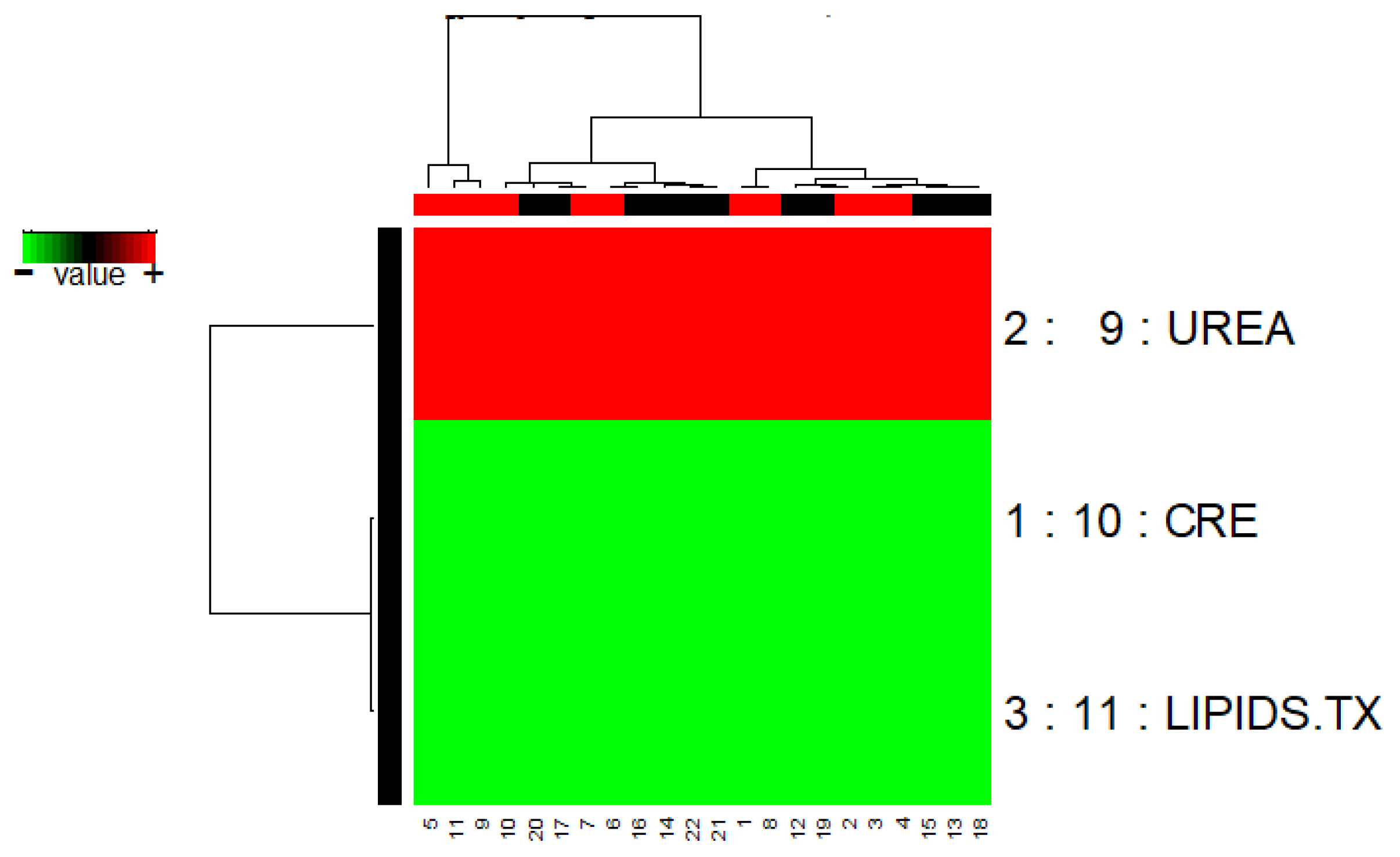
3.1.3. GALGO
3.1.4. Elastic Net
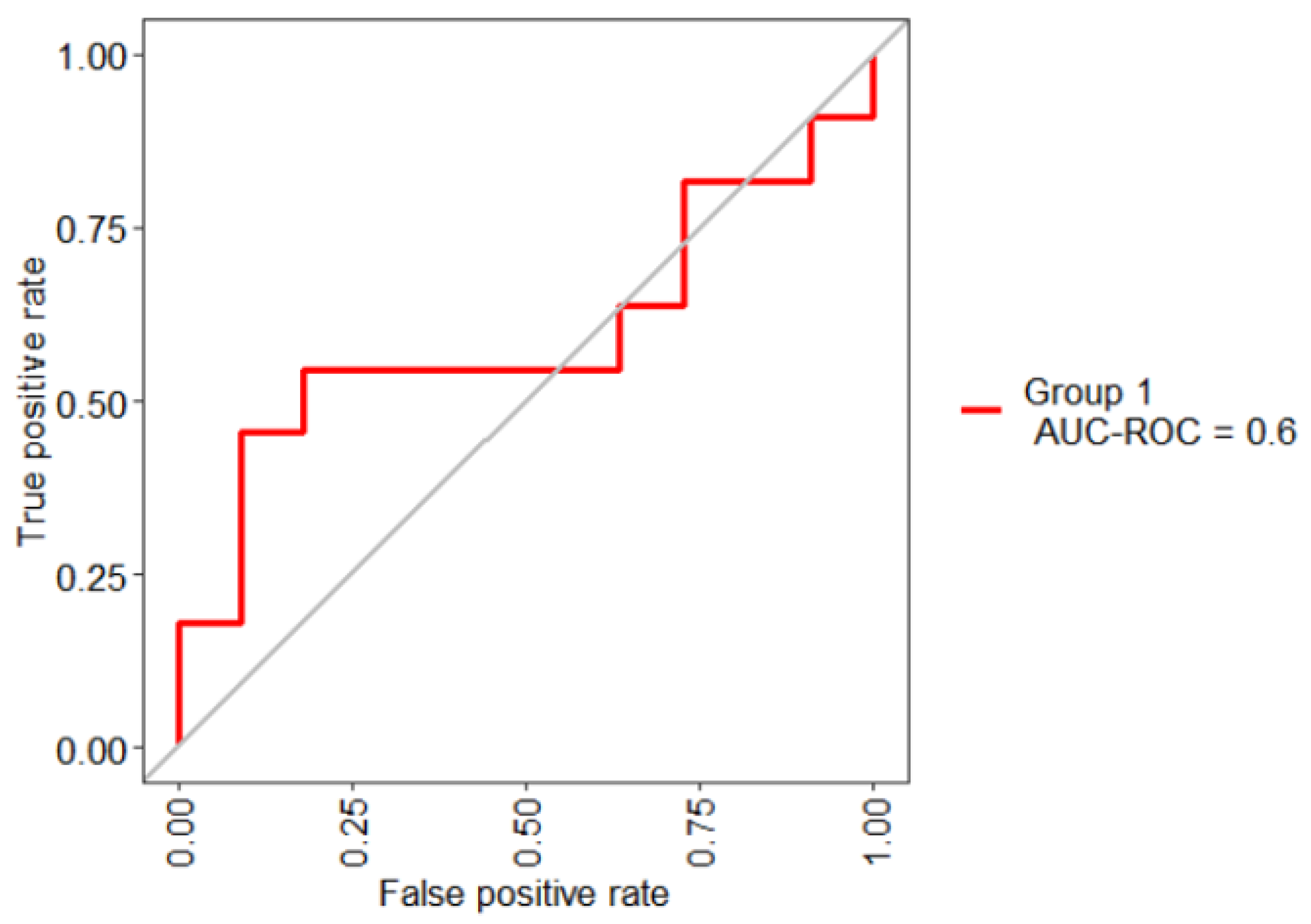
3.2. Classification Performance
- Bad test = [0.5, 0.6)
- Regular test = [0.6, 0.75)
- Good test = [0.75, 0.9)
- Very good test = [0.9, 0.97)
- Excellent test = [0.97, 1)
- Model 1. “feature obtained by Boruta [CRE]” + RF
- Model 2. “features obtained by GALGO [CRE, UREA and LIPIDS.TX]” + RF
- Model 3. “features obtained by Elastic net [AGE, UREA, CRE, LIPIDS.TX, GFR and GB]” + RF
- Model 4. “features obtained by UFS [GLU, UREA, CRE, TCHOLU, UTG, GFR, and GB]” + RF
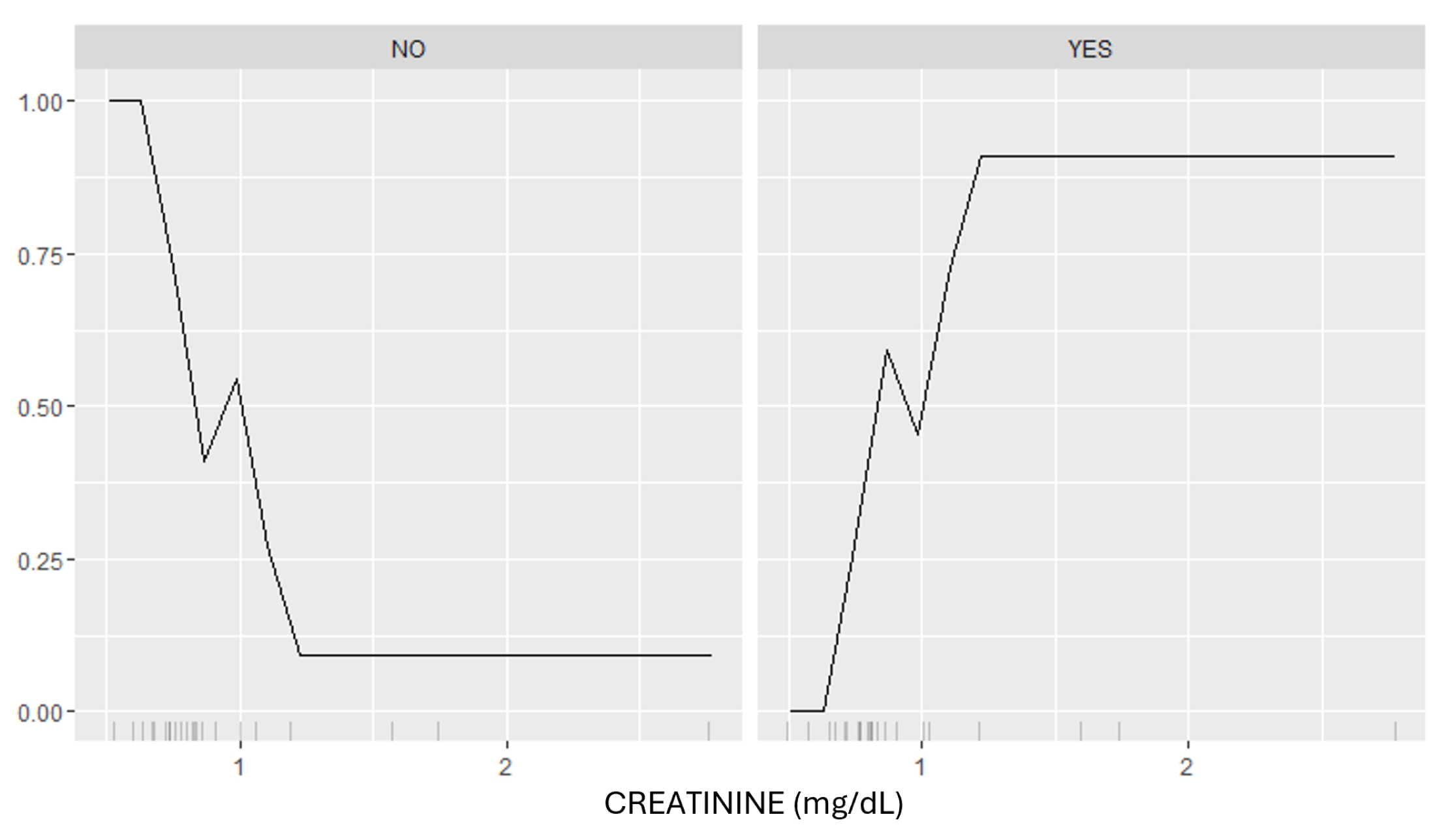
3.3. Model Interpretation
4. Discussion and Conclusions
Author Contributions
Funding
Institutional Review Board Statement
Informed Consent Statement
Data Availability Statement
Conflicts of Interest
References
- Atlas, I. IDF Diabetes Atlas, 10th ed.; International Diabetes Federation: Brussels, Belgium, 2021. [Google Scholar]
- Saeedi, P.; Petersohn, I.; Salpea, P.; Malanda, B.; Karuranga, S.; Unwin, N.; Colagiuri, S.; Guariguata, L.; Motala, A.A.; Ogurtsova, K.; et al. Global and regional diabetes prevalence estimates for 2019 and projections for 2030 and 2045: Results from the International Diabetes Federation Diabetes Atlas. Diabetes Res. Clin. Pract. 2019, 157, 107843. [Google Scholar] [CrossRef] [PubMed]
- Barengo, N.C.; Apolinar, L.M.; Estrada Cruz, N.A.; Fernández Garate, J.E.; Correa González, R.A.; Diaz Valencia, P.A.; Gonzalez, C.A.C.; Rodriguez, J.A.G.; González, N.C. Development of an information system and mobile application for the care of type 2 diabetes patients at the primary care level for the health sector in Mexico: Study protocol for a randomized controlled, open-label trial. Trials 2022, 23, 253. [Google Scholar] [CrossRef]
- Liu, X.z.; Duan, M.; Huang, H.d.; Zhang, Y.; Xiang, T.y.; Niu, W.c.; Zhou, B.; Wang, H.l.; Zhang, T.t. Predicting diabetic kidney disease for type 2 diabetes mellitus by machine learning in the real world: A multicenter retrospective study. Front. Endocrinol. 2023, 14, 1184190. [Google Scholar] [CrossRef] [PubMed]
- Huang, G.M.; Huang, K.Y.; Lee, T.Y.; Weng, J.T.Y. An interpretable rule-based diagnostic classification of diabetic nephropathy among type 2 diabetes patients. BMC Bioinform. 2015, 16, S5. [Google Scholar] [CrossRef] [PubMed]
- Yokoyama, H.; Araki, S.i.; Honjo, J.; Okizaki, S.; Yamada, D.; Shudo, R.; Shimizu, H.; Sone, H.; Moriya, T.; Haneda, M. Association between remission of macroalbuminuria and preservation of renal function in patients with type 2 diabetes with overt proteinuria. Diabetes Care 2013, 36, 3227–3233. [Google Scholar] [CrossRef] [PubMed]
- Atlas, I. IDF Diabetes Atlas, 9th ed.; International Diabetes Federation: Brussels, Belgium, 2019. [Google Scholar]
- Vázquez-Moreno, M.; Locia-Morales, D.; Peralta-Romero, J.; Sharma, T.; Meyre, D.; Cruz, M.; Flores-Alfaro, E.; Valladares-Salgado, A. AGT rs4762 is associated with diastolic blood pressure in Mexicans with diabetic nephropathy. J. Diabetes Its Complicat. 2021, 35, 107826. [Google Scholar] [CrossRef]
- Samsu, N. Diabetic nephropathy: Challenges in pathogenesis, diagnosis, and treatment. BioMed Res. Int. 2021, 2021, 1497449. [Google Scholar] [CrossRef] [PubMed]
- Basuli, D.; Kavcar, A.; Roy, S. From bytes to nephrons: AI’s journey in diabetic kidney disease. J. Nephrol. 2024, 1–11. [Google Scholar] [CrossRef] [PubMed]
- Afsaneh, E.; Sharifdini, A.; Ghazzaghi, H.; Ghobadi, M.Z. Recent applications of machine learning and deep learning models in the prediction, diagnosis, and management of diabetes: A comprehensive review. Diabetol. Metab. Syndr. 2022, 14, 196. [Google Scholar] [CrossRef]
- Vijayan, V.V.; Anjali, C. Prediction and diagnosis of diabetes mellitus—A machine learning approach. In Proceedings of the 2015 IEEE Recent Advances in Intelligent Computational Systems (RAICS), Trivandrum, India, 10–12 December 2015; pp. 122–127. [Google Scholar]
- Zou, Q.; Qu, K.; Luo, Y.; Yin, D.; Ju, Y.; Tang, H. Predicting diabetes mellitus with machine learning techniques. Front. Genet. 2018, 9, 515. [Google Scholar] [CrossRef]
- Fatima, M.; Pasha, M. Survey of machine learning algorithms for disease diagnostic. J. Intell. Learn. Syst. Appl. 2017, 9, 1–16. [Google Scholar] [CrossRef]
- Tuppad, A.; Patil, S.D. Machine learning for diabetes clinical decision support: A review. Adv. Comput. Intell. 2022, 2, 22. [Google Scholar] [CrossRef]
- Nagarajan, S.M.; Muthukumaran, V.; Murugesan, R.; Joseph, R.B.; Meram, M.; Prathik, A. Innovative feature selection and classification model for heart disease prediction. J. Reliab. Intell. Environ. 2022, 8, 333–343. [Google Scholar] [CrossRef]
- Nagarajan, S.M.; Deverajan, G.G.; Chatterjee, P.; Alnumay, W.; Ghosh, U. Effective task scheduling algorithm with deep learning for Internet of Health Things (IoHT) in sustainable smart cities. Sustain. Cities Soc. 2021, 71, 102945. [Google Scholar] [CrossRef]
- Chang, V.; Bailey, J.; Xu, Q.A.; Sun, Z. Pima Indians diabetes mellitus classification based on machine learning (ML) algorithms. Neural Comput. Appl. 2023, 35, 16157–16173. [Google Scholar] [CrossRef]
- Usman, T.M.; Saheed, Y.K.; Ignace, D.; Nsang, A. Diabetic retinopathy detection using principal component analysis multi-label feature extraction and classification. Int. J. Cogn. Comput. Eng. 2023, 4, 78–88. [Google Scholar] [CrossRef]
- Rodriguez-Romero, V.; Bergstrom, R.F.; Decker, B.S.; Lahu, G.; Vakilynejad, M.; Bies, R.R. Prediction of nephropathy in type 2 diabetes: An analysis of the ACCORD trial applying machine learning techniques. Clin. Transl. Sci. 2019, 12, 519–528. [Google Scholar] [CrossRef]
- Jiang, S.; Fang, J.; Yu, T.; Liu, L.; Zou, G.; Gao, H.; Zhuo, L.; Li, W. Novel model predicts diabetic nephropathy in type 2 diabetes. Am. J. Nephrol. 2020, 51, 130–138. [Google Scholar] [CrossRef] [PubMed]
- Shi, R.; Niu, Z.; Wu, B.; Zhang, T.; Cai, D.; Sun, H.; Hu, Y.; Mo, R.; Hu, F. Nomogram for the risk of diabetic nephropathy or diabetic Retinopathy among patients with type 2 diabetes mellitus based on questionnaire and biochemical indicators: A cross-sectional study. Diabetes Metab. Syndr. Obes. Targets Ther. 2020, 13, 1215. [Google Scholar] [CrossRef]
- Xi, C.; Wang, C.; Rong, G.; Deng, J. A nomogram model that predicts the risk of diabetic nephropathy in type 2 diabetes mellitus patients: A retrospective study. Int. J. Endocrinol. 2021, 2021, 6672444. [Google Scholar] [CrossRef] [PubMed]
- Maniruzzaman, M.; Islam, M.M.; Rahman, M.J.; Hasan, M.A.M.; Shin, J. Risk prediction of diabetic nephropathy using machine learning techniques: A pilot study with secondary data. Diabetes Metab. Syndr. Clin. Res. Rev. 2021, 15, 102263. [Google Scholar] [CrossRef]
- Yang, J.; Jiang, S. Development and Validation of a Model That Predicts the Risk of Diabetic Nephropathy in Type 2 Diabetes Mellitus Patients: A Cross-Sectional Study. Int. J. Gen. Med. 2022, 15, 5089. [Google Scholar] [CrossRef] [PubMed]
- Jović, A.; Brkić, K.; Bogunović, N. A review of feature selection methods with applications. In Proceedings of the 2015 38th International Convention on Information and Communication Technology, Electronics and Microelectronics (MIPRO), Opatija, Croatia, 25–29 May 2015; pp. 1200–1205. [Google Scholar]
- Lopez-Rincon, A.; Martinez-Archundia, M.; Martinez-Ruiz, G.U.; Schoenhuth, A.; Tonda, A. Automatic discovery of 100-miRNA signature for cancer classification using ensemble feature selection. BMC Bioinform. 2019, 20, 480. [Google Scholar] [CrossRef] [PubMed]
- Ahmadpour, H.; Bazrafshan, O.; Rafiei-Sardooi, E.; Zamani, H.; Panagopoulos, T. Gully erosion susceptibility assessment in the Kondoran watershed using machine learning algorithms and the Boruta feature selection. Sustainability 2021, 13, 10110. [Google Scholar] [CrossRef]
- Trevino, V.; Falciani, F. GALGO: An R package for multivariate variable selection using genetic algorithms. Bioinformatics 2006, 22, 1154–1156. [Google Scholar] [CrossRef]
- Liu, Y.; Gopalakrishnan, V. An overview and evaluation of recent machine learning imputation methods using cardiac imaging data. Data 2017, 2, 8. [Google Scholar] [CrossRef] [PubMed]
- Kursa, M.B.; Rudnicki, W.R. Feature selection with the Boruta package. J. Stat. Softw. 2010, 36, 1–13. [Google Scholar] [CrossRef]
- Kursa, M.B.; Jankowski, A.; Rudnicki, W.R. Boruta–a system for feature selection. Fundam. Inform. 2010, 101, 271–285. [Google Scholar] [CrossRef]
- Zou, H.; Hastie, T. Regularization and variable selection via the elastic net. J. R. Stat. Soc. Ser. B (Stat. Methodol.) 2005, 67, 301–320. [Google Scholar] [CrossRef]
- Alrashdi, A.M.; Atitallah, I.B.; Al-Naffouri, T.Y. Precise performance analysis of the box-elastic net under matrix uncertainties. IEEE Signal Process. Lett. 2019, 26, 655–659. [Google Scholar] [CrossRef]
- Breiman, L. Random forests. Mach. Learn. 2001, 45, 5–32. [Google Scholar] [CrossRef]
- Svetnik, V.; Liaw, A.; Tong, C.; Culberson, J.C.; Sheridan, R.P.; Feuston, B.P. Random forest: A classification and regression tool for compound classification and QSAR modeling. J. Chem. Inf. Comput. Sci. 2003, 43, 1947–1958. [Google Scholar] [CrossRef]
- Parikh, R.; Mathai, A.; Parikh, S.; Sekhar, G.C.; Thomas, R. Understanding and using sensitivity, specificity and predictive values. Indian J. Ophthalmol. 2008, 56, 45. [Google Scholar] [CrossRef] [PubMed]
- Fawcett, T. An introduction to ROC analysis. Pattern Recognit. Lett. 2006, 27, 861–874. [Google Scholar] [CrossRef]
- Rakotomamonjy, A. Optimizing Area Under Roc Curve with SVMs. In Proceedings of the ROC Analysis in Artificial Intelligence, 1st International Workshop, ROCAI-2004, Valencia, Spain, 22 August 2004; pp. 71–80. [Google Scholar]
- Kohavi, R. A study of cross-validation and bootstrap for accuracy estimation and model selection. In Proceedings of the IJCAI’95: 14th International Joint Conference on Artificial Intelligence, Montreal, QC, Canada, 20–25 August 1995; Volume 14, pp. 1137–1145. [Google Scholar]
- Lundberg, S. A unified approach to interpreting model predictions. arXiv 2017, arXiv:1705.07874. [Google Scholar]
- Ghosh, S.K.; Khandoker, A.H. Investigation on explainable machine learning models to predict chronic kidney diseases. Sci. Rep. 2024, 14, 3687. [Google Scholar] [CrossRef] [PubMed]
- Ahmad, M.A.; Eckert, C.; Teredesai, A. Interpretable machine learning in healthcare. In Proceedings of the 2018 ACM International Conference on Bioinformatics, Computational Biology, and Health Informatics, New York, NY, USA, 4–7 June 2018; pp. 559–560. [Google Scholar]
- John, C.R. MLeval: Machine Learning Model Evaluation, R package version 0.3; 2020. Available online: https://cran.r-project.org/package=MLeval (accessed on 1 September 2024).
- Friedman, J.; Hastie, T.; Tibshirani, R. Regularization paths for generalized linear models via coordinate descent. J. Stat. Softw. 2010, 33, 1–22. [Google Scholar] [CrossRef] [PubMed]
- Kuhn, M. caret: Classification and Regression Training, R package version 6.0-86; 2020. Available online: https://cran.r-project.org/package=caret (accessed on 1 September 2024).
- Molnar, C.; Casalicchio, G.; Bischl, B. iml: An R package for interpretable machine learning. J. Open Source Softw. 2018, 3, 786. [Google Scholar] [CrossRef]
- Sun, L.; Wang, J.; Wei, J. AVC: Selecting discriminative features on basis of AUC by maximizing variable complementarity. BMC Bioinform. 2017, 18, 73–89. [Google Scholar] [CrossRef] [PubMed]
- Martínez-Torteya, A.; Treviño, V.; Tamez-Peña, J.G. Improved diagnostic multimodal biomarkers for Alzheimer’s disease and mild cognitive impairment. BioMed Res. Int. 2015, 2015, 961314. [Google Scholar] [CrossRef] [PubMed]
- Zhang, Z.; Trevino, V.; Hoseini, S.S.; Belciug, S.; Boopathi, A.M.; Zhang, P.; Gorunescu, F.; Subha, V.; Dai, S. Variable selection in Logistic regression model with genetic algorithm. Ann. Transl. Med. 2018, 6, 45. [Google Scholar] [CrossRef] [PubMed]
- Wu, C.C.; Yeh, W.C.; Hsu, W.D.; Islam, M.M.; Nguyen, P.A.A.; Poly, T.N.; Wang, Y.C.; Yang, H.C.; Li, Y.C.J. Prediction of fatty liver disease using machine learning algorithms. Comput. Methods Programs Biomed. 2019, 170, 23–29. [Google Scholar] [CrossRef] [PubMed]
- Ganggayah, M.D.; Taib, N.A.; Har, Y.C.; Lio, P.; Dhillon, S.K. Predicting factors for survival of breast cancer patients using machine learning techniques. BMC Med. Inform. Decis. Mak. 2019, 19, 48. [Google Scholar] [CrossRef] [PubMed]
- Lebedev, A.; Westman, E.; Van Westen, G.; Kramberger, M.; Lundervold, A.; Aarsland, D.; Soininen, H.; Kłoszewska, I.; Mecocci, P.; Tsolaki, M.; et al. Random Forest ensembles for detection and prediction of Alzheimer’s disease with a good between-cohort robustness. NeuroImage Clin. 2014, 6, 115–125. [Google Scholar] [CrossRef] [PubMed]
- Cui, M.; Gang, X.; Gao, F.; Wang, G.; Xiao, X.; Li, Z.; Li, X.; Ning, G.; Wang, G. Risk assessment of sarcopenia in patients with type 2 diabetes mellitus using data mining methods. Front. Endocrinol. 2020, 11, 123. [Google Scholar] [CrossRef] [PubMed]
- Lasko, T.A.; Bhagwat, J.G.; Zou, K.H.; Ohno-Machado, L. The use of receiver operating characteristic curves in biomedical informatics. J. Biomed. Inform. 2005, 38, 404–415. [Google Scholar] [CrossRef] [PubMed]
- Villagrana-Bañuelos, K.E.; Maeda-Gutiérrez, V.; Alcalá-Rmz, V.; Oropeza-Valdez, J.J.; Oostdam, H.V.; Ana, S.; Castañeda-Delgado, J.E.; López, J.A.; Borrego Moreno, J.C.; Galván-Tejada, C.E.; et al. COVID-19 outcome prediction by integrating clinical and metabolic data using machine learning algorithms. Rev. Investig. Clínica 2022, 74, 314–327. [Google Scholar] [CrossRef]
- Dabla, P.K. Renal function in diabetic nephropathy. World J. Diabetes 2010, 1, 48. [Google Scholar] [CrossRef]
- Currie, G.; McKay, G.; Delles, C. Biomarkers in diabetic nephropathy: Present and future. World J. Diabetes 2014, 5, 763. [Google Scholar] [CrossRef]
- Campion, C.G.; Sanchez-Ferras, O.; Batchu, S.N. Potential role of serum and urinary biomarkers in diagnosis and prognosis of diabetic nephropathy. Can. J. Kidney Health Dis. 2017, 4, 2054358117705371. [Google Scholar] [CrossRef]
- Lim, A.K.; Tesch, G.H. Inflammation in diabetic nephropathy. Mediat. Inflamm. 2012, 2012, 146154. [Google Scholar] [CrossRef] [PubMed]
- Shang, J.; Wang, L.; Zhang, Y.; Zhang, S.; Ning, L.; Zhao, J.; Cheng, G.; Liu, D.; Xiao, J.; Zhao, Z. Chemerin/ChemR23 axis promotes inflammation of glomerular endothelial cells in diabetic nephropathy. J. Cell. Mol. Med. 2019, 23, 3417–3428. [Google Scholar] [CrossRef] [PubMed]
- Valensi, P.; Picard, S. Lipids, lipid-lowering therapy and diabetes complications. Diabetes Metab. 2011, 37, 15–24. [Google Scholar] [CrossRef] [PubMed]
- Ayodele, O.E.; Alebiosu, C.O.; Salako, B.L. Diabetic nephropathy–a review of the natural history, burden, risk factors and treatment. J. Natl. Med Assoc. 2004, 96, 1445. [Google Scholar]
- Lin, P.H.; Duann, P. Dyslipidemia in kidney disorders: Perspectives on mitochondria homeostasis and therapeutic opportunities. Front. Physiol. 2020, 11, 1050. [Google Scholar] [CrossRef] [PubMed]
- Mitrofanova, A.; Merscher, S.; Fornoni, A. Kidney lipid dysmetabolism and lipid droplet accumulation in chronic kidney disease. Nat. Rev. Nephrol. 2023, 19, 629–645. [Google Scholar] [CrossRef] [PubMed]


| Author’s and Year | Feature Selection Method | Risk Factors | Classification Algorithm |
|---|---|---|---|
| Rodriguez-Romero et al. 2019 [20] | InfoGain | Age Cholesterol Triglycerides Low-density lipoprotein Urinary albumin excretion Glomerular filtrarion rate | 1R J48 RF SL SMO NB |
| Jiang et al. 2020 [21] | LASSO | DR HbA1c Gender Anemia Hemateuria DM duration Blood pressure Urinary protein excretion Estimated glomerular filtrarion rate | LR |
| Shi et al. 2020 [22] | LASSO LR | HbA1c Disease course Body mass index Total triglycerides Blood urea nitrogen Systolic blood pressure Postprandial blood glucose | LR |
| Xi et al. 2021 [23] | LASSO LR | Age Gender Hypertension Medicine use Duration of DM Body mass index Serum creatinine level Blood urea nitrogen level Neutrophil to lympocyte ratio Red blood cell distribution width | LR |
| Maniruzzaman et al. 2021 [24] | PCA | Age HbA1c Triglycerides DM duration Body mass index Fasting blood sugar Low density lipoprotein High density lipoprotein Systolic blood pressure Diastolic blood pressure | LDA SVM LR K-NN NB ANN |
| Yang and Jiang 2022 [25] | Univariate AIC | HbA1c Triglycerides Hypertension Serum creatinine Body mass index Blood urea nitrogen Diabetic peripheral neuropathy | LR |
| Predictors (n = 32) | Cases (n = 11) | Controls (n = 11) | p-Value |
|---|---|---|---|
| Demographic Characteristics | |||
| EDU | |||
| 1—Elementary school 2—Secondary school 3—Technical school 4—High school 5—Professional 6—Postgraduate | 2 (18.18%) 3 (27.27%) 2 (18.18%) - 4 (36.36%) - | 1 (9.09%) 2 (18.18%) 2 (18.18%) 3 (27.27%) 3 (27.27%) - | 0.559 |
| SAL | |||
| 1—Less than 2000.00 MXN (~98.16 USD) 2—Between 2000.00 and 5000.00 MXN (~98.16–245.39 USD) 3—More than 5000.00 MXN (~245.39 USD) | 3 (27.27%) 3 (27.27%) 5 (45.45%) | 3 (27.27%) 2 (18.18%) 6 (54.54%) | 0.409 |
| SEX | |||
| 0—Male 1—Female | 6 (54.54%) 5 (45.45%) | 6 (54.54%) 5 (45.45%) | 1 |
| AGE, years | 62.909 (±11.597) | 52.909 (±12.045) | 0.0816 |
| AGE DX, years | 45.636 (±6.561) | 45.272 (±11.199) | 0.922 |
| Clinical observations | |||
| WHR, cm/cm | 0.963 (±0.092) | 0.914 (±0.094) | 0.233 |
| BMI kg/m2 | 30.486 (±3.685) | 29.225 (±7.205) | 0.591 |
| SBP, mmHg | 125.909 (±15.623) | 1223.636 (±15.666) | 0.722 |
| DBP, mmHg | 82.727 (±9.045) | 79.545 (±8.790) | 0.395 |
| USBP, mmHg | 122.272 (±12.915) | 120.909 (±12.21) | 0.79 |
| UDBP, mmHg | 80.909 (±8.312) | 78.181 (±7.507) | 0.413 |
| GLU, mg/dL | 127.363 (±43.845) | 167.363 (±78.888) | 0.159 |
| UREA, mg/dL | 45.818 (±25.732) | 28 (±7.835) | 0.1082 |
| CRE, mg/dL | 1.196 (±0.622) | 0.733 (±0.136) | 0.074 |
| CHOL, mg/dL | 222.518 (±74.48) | 206.663 (±58.252) | 0.475 |
| HDL, mg/dL | 37.881 (±10.939) | 40.136 (±14.742) | 0.672 |
| LDL, mg/dL | 161.045 (±67.839) | 136.055 (±37.055) | 0.294 |
| TG, mg/dL | 247.427 (±162.302) | 310.536 (±274.891) | 0.503 |
| TCHOLU, mg/dL | 193.909 (±69.288) | 193 (±41.916) | 0.969 |
| UHDL, mg/dL | 41.639 (±9.982) | 41.0909 (±14.117) | 0.913 |
| ULDL, mg/dL | 130.181 (±60.237) | 123.545 (±22.979) | 0.722 |
| UTG, mg/dL | 211.090 (±151.341) | 302 (±260.799) | 0.325 |
| HBA1C, mmol/L | 6.994 (±2.527) | 8.209 (±2.667) | 0.28 |
| GFR | 76.807 (±28.853) | 111.454 (±44.331) | 0.0583 |
| Medical treatment | |||
| LIPIDS-TX | |||
| 0—No 1—Yes | 4 (36.36%) 7 (63.63%) | 8 (72.72%) 3 (27.27%) | 0.095 |
| HA-TX | |||
| 0—No 1—Yes | 7 (63.63%) 4 (36.36%) | 8 (72.72%) 3 (27.27%) | 0.48 |
| GB | |||
| 0—No 1—Yes | 6 (54.54%) 5 (45.45%) | 10 (90.90%) 1 (9.09%) | 0.08 |
| MF | |||
| 0—No 1—Yes | 3 (27.27%) 8 (72.72%) | 3 (27.27%) 8 (72.72%) | 1 |
| PG | |||
| 0—No 1—Yes | 11 (100%) - | 11 (100%) - | - |
| RG | |||
| 0—No 1—Yes | 11 (100%) - | 11 (100%) - | - |
| AB | |||
| 0—No 1—Yes | 11 (100%) - | 11 (100%) - | - |
| INS | |||
| 0—No 1—Yes | 8 (72.72%) 3 (27.27%) | 6 (54.54%) 5 (45.45%) | 0.379 |
| Feature | AUC Value | Feature | AUC Value |
|---|---|---|---|
| EDU | 0.29 | LDL | 0.29 |
| SAL | 0.55 | TG | 0.50 |
| SEX | 0.26 | TCHOLU | 0.64 |
| AGE | 0.53 | UHDL | 0.58 |
| AGE DX | 0.47 | ULDL | 0.55 |
| WHR | 0.25 | UTG | 0.67 |
| BMI | 0.57 | HBA1C | 0.46 |
| SBP | 0.13 | GFR | 0.68 |
| DBP | 0.28 | GB | 0.60 |
| USBP | 0.40 | MF | 0.16 |
| UDBP | 0.41 | PG | - |
| GLU | 0.67 | RG | - |
| UREA | 0.60 | AB | - |
| CRE | 0.61 | INS | 0.45 |
| CHOL | 0.53 | LIPIDS.TX | 0.48 |
| HDL | 0.44 | HA TX | 0.24 |
| Attribute | meanImp | medianImp | minImp | maxImp | normHits | Decision |
|---|---|---|---|---|---|---|
| EDU | −0.68 | −1.02 | −2.07 | 1.73 | 0.00 | Rejected |
| SAL | 0.23 | 0.18 | −1.81 | 2.00 | 0.00 | Rejected |
| SEX | −0.44 | −0.725 | −1.69 | 1.41 | 0.00 | Rejected |
| AGE | 0.81 | 1.04 | −0.99 | 2.05 | 0.00 | Rejected |
| AGE DX | 0.01 | 0.21 | −1.96 | 1.93 | 0.00 | Rejected |
| WHR | −1.10 | −1.36 | −2.14 | 0.80 | 0.00 | Rejected |
| BMI | 0.05 | 0.09 | −1.01 | 1.20 | 0.00 | Rejected |
| GLU | 3.01 | 2.98 | −0.65 | 6.61 | 0.46 | Tentative |
| UREA | 0.92 | 0.96 | −1.07 | 2.34 | 0.00 | Rejected |
| CRE | 6.69 | 6.83 | 2.16 | 9.81 | 0.85 | Confirmed |
| LIPIDS-TX | 0.12 | 0.12 | −2.07 | 2.23 | 0.00 | Rejected |
| CHOL | −0.02 | 0.37 | −2.90 | 1.16 | 0.00 | Rejected |
| HDL | −0.43 | −0.38 | −2.20 | 1.56 | 0.00 | Rejected |
| LDL | −1.00 | −0.96 | −2.13 | 0.07 | 0.00 | Rejected |
| TG | −0.72 | −0.59 | −2.60 | 1.10 | 0.00 | Rejected |
| TCHOLU | −0.54 | −0.98 | −2.66 | 1.76 | 0.00 | Rejected |
| UHDL | −1.08 | −1.06 | −3.28 | 0.42 | 0.00 | Rejected |
| ULDL | 0.01 | −0.01 | −2.70 | 2.11 | 0.00 | Rejected |
| UTG | −1.08 | −0.98 | −2.32 | −0.16 | 0.00 | Rejected |
| HA-TX | −0.56 | −0.95 | −1.62 | 1.38 | 0.00 | Rejected |
| SBP | −0.81 | −0.74 | −2.47 | 1.41 | 0.00 | Rejected |
| DBP | −0.81 | −0.89 | −2.08 | 0.63 | 0.00 | Rejected |
| USBP | −1.03 | −1.25 | −2.13 | 0.48 | 0.00 | Rejected |
| UDBP | −0.51 | −0.46 | −1.66 | 0.75 | 0.00 | Rejected |
| HBA1C | 0.08 | 0.15 | −1.46 | 2.21 | 0.00 | Rejected |
| GFR | 2.95 | 3.00 | −0.75 | 7.23 | 0.48 | Tentative |
| GB | 0.13 | −0.22 | −1.16 | 2.05 | 0.00 | Rejected |
| MF | −0.92 | −1.00 | −2.08 | 1.00 | 0.00 | Rejected |
| PG | 0.00 | 0.00 | 0.00 | 0.00 | 0.00 | Rejected |
| RG | 0.00 | 0.00 | 0.00 | 0.00 | 0.00 | Rejected |
| AB | 0.00 | 0.00 | 0.00 | 0.00 | 0.00 | Rejected |
| INS | −0.75 | −0.85 | −1.72 | 0.87 | 0.00 | Rejected |
| Parameter | Description | Value |
|---|---|---|
| Classification method | Method used for classification | RF |
| Chromosome size | Number of variables include in each model | 5 |
| Max solutions | A collection of solutions desired | 50 |
| Max generations | Number of generations that GA can evolve | 300 |
| Goal fitness | Desired fitness value | 1.0 |
| Features | Coefficients |
|---|---|
| AGE | 0.010 |
| UREA | 0.001 |
| CRE | 0.494 |
| LIPIDS-TX | 0.406 |
| GFR | −0.004 |
| GB | 0.310 |
| AUC | SN | SP |
|---|---|---|
| 0.60 | 0.545 | 0.455 |
| Feature Selection Method | Features Number | Features | AUC | SN | SP |
|---|---|---|---|---|---|
| Boruta | 1 | CRE | 0.61 | 0.455 | 0.636 |
| Galgo | 3 | CRE UREA LIPIDS.TX | 0.80 | 0.909 | 0.818 |
| Elastic net | 6 | AGE UREA CRE LIPIDS.TX GFR GB | 0.75 | 0.720 | 0.720 |
| Multivariate | 7 | GLU UREA CRE TCHOLU UTG GFR GB | 0.74 | 0.636 | 0.545 |
| LOOCV + (3 FEAT [GALGO]) RF | LOOCV + (3 FEAT [GALGO]) SVM | ||||
|---|---|---|---|---|---|
| AUC | SN | SP | AUC | SN | SP |
| 0.790 | 0.818 | 0.818 | 0.760 | 0.727 | 0.818 |
| k = 10 CV + (3 FEAT [GALGO]) RF | k = 10 CV + (3 FEAT [GALGO]) SVM | ||||
| AUC | SN | SP | AUC | SN | SP |
| 0.800 | 0.909 | 0.818 | 0.750 | 0.727 | 0.727 |
| Author’s and Year | Feature Selection Method | # of Features | Classification Algorithm | Evaluation Metrics |
|---|---|---|---|---|
| Rodriguez-Romero et al. 2019 [20] | InfoGain | 6 | 1R J48 RF SL SMO NB | SN: 0.871; SP: 0.979; ACC: 0.871 SN: 0.887; SP: 0.249; ACC: 0.887 SN: 0.887; SP: 0.999; ACC: 0.887 SN: 0.899; SP: 0.183; ACC: 0.899 SN: 0.893; SP: 0.159; ACC: 0.893 SN: 0.804; SP: 0.355; ACC: 0.803 |
| Jiang et al. 2020 [21] | LASSO | 9 | LR | C-INDEX: 0.934 |
| Shi et al. 2020 [22] | LASSO LR | 10 | LR | AUC: 0.807; C-INDEX: 0.807 |
| Xi et al. 2021 [23] | LASSO LR | 10 | LR | AUC: 0.813; C-INDEX: 0.819 |
| Maniruzzaman et al. 2021 [24] | PCA | 10 | LDA SVM-RBF LR KNN NB ANN | AUC: 0.880; SN: 0.867; SP: 0.852 AUC: 0.910; SN: 0.867; SP: 0.863 AUC: 0.890; SN: 0.800; SP: 0.823 AUC: 0.890; SN: 0.833; SP: 0.849 AUC: 0.900; SN: 0.717; SP: 0.904 AUC: 0.900; SN: 0.800; SP: 0.823 |
| Yang and Jiang 2022 [25] | Univariate AIC | 7 | LR | AUC: 0.758; C-INDEX: 0.758 |
| Proposed | GALGO | 3 | RF | AUC: 0.800; SN: 0.909; SP: 0.818 |
Disclaimer/Publisher’s Note: The statements, opinions and data contained in all publications are solely those of the individual author(s) and contributor(s) and not of MDPI and/or the editor(s). MDPI and/or the editor(s) disclaim responsibility for any injury to people or property resulting from any ideas, methods, instructions or products referred to in the content. |
© 2024 by the authors. Licensee MDPI, Basel, Switzerland. This article is an open access article distributed under the terms and conditions of the Creative Commons Attribution (CC BY) license (https://creativecommons.org/licenses/by/4.0/).
Share and Cite
Maeda-Gutiérrez, V.; Galván-Tejada, C.E.; Galván-Tejada, J.I.; Cruz, M.; Celaya-Padilla, J.M.; Gamboa-Rosales, H.; García-Hernández, A.; Luna-García, H.; Villalba-Condori, K.O. Evaluating Feature Selection Methods for Accurate Diagnosis of Diabetic Kidney Disease. Biomedicines 2024, 12, 2858. https://doi.org/10.3390/biomedicines12122858
Maeda-Gutiérrez V, Galván-Tejada CE, Galván-Tejada JI, Cruz M, Celaya-Padilla JM, Gamboa-Rosales H, García-Hernández A, Luna-García H, Villalba-Condori KO. Evaluating Feature Selection Methods for Accurate Diagnosis of Diabetic Kidney Disease. Biomedicines. 2024; 12(12):2858. https://doi.org/10.3390/biomedicines12122858
Chicago/Turabian StyleMaeda-Gutiérrez, Valeria, Carlos E. Galván-Tejada, Jorge I. Galván-Tejada, Miguel Cruz, José M. Celaya-Padilla, Hamurabi Gamboa-Rosales, Alejandra García-Hernández, Huizilopoztli Luna-García, and Klinge Orlando Villalba-Condori. 2024. "Evaluating Feature Selection Methods for Accurate Diagnosis of Diabetic Kidney Disease" Biomedicines 12, no. 12: 2858. https://doi.org/10.3390/biomedicines12122858
APA StyleMaeda-Gutiérrez, V., Galván-Tejada, C. E., Galván-Tejada, J. I., Cruz, M., Celaya-Padilla, J. M., Gamboa-Rosales, H., García-Hernández, A., Luna-García, H., & Villalba-Condori, K. O. (2024). Evaluating Feature Selection Methods for Accurate Diagnosis of Diabetic Kidney Disease. Biomedicines, 12(12), 2858. https://doi.org/10.3390/biomedicines12122858