
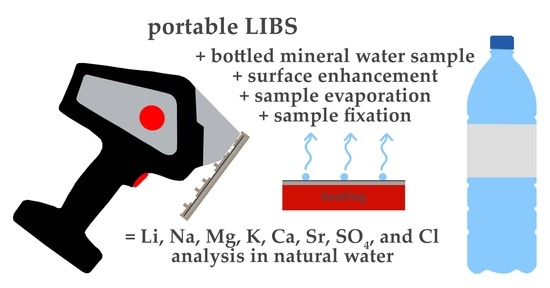
Utilising Portable Laser-Induced Breakdown Spectroscopy for Quantitative Inorganic Water Testing


Abstract
:
1. Introduction
2. Materials and Methods
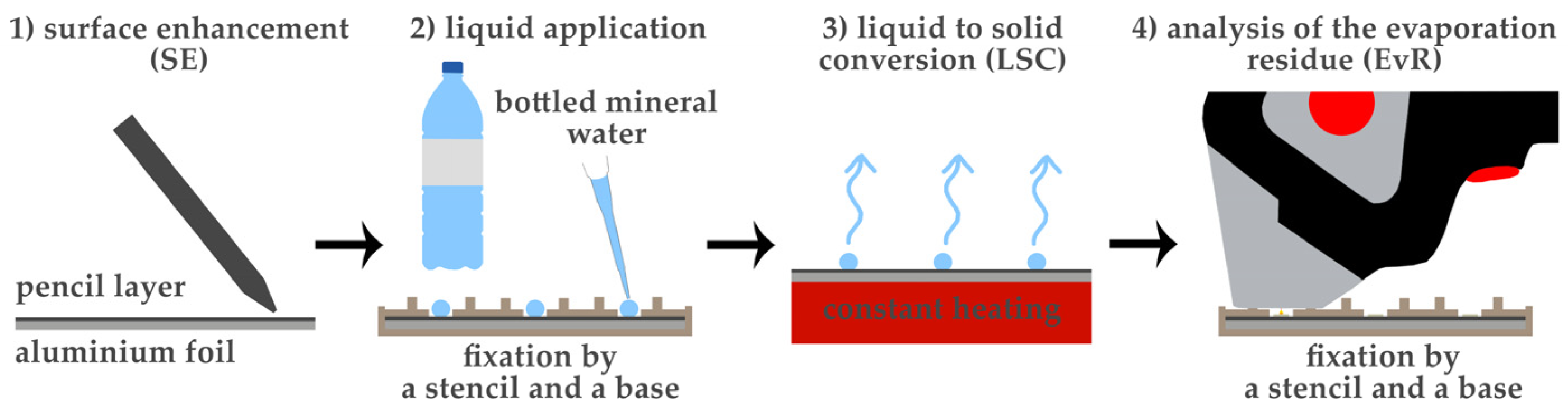
2.1. Sample Preparation
2.2. Instrumentation
2.3. Liquid Analysis
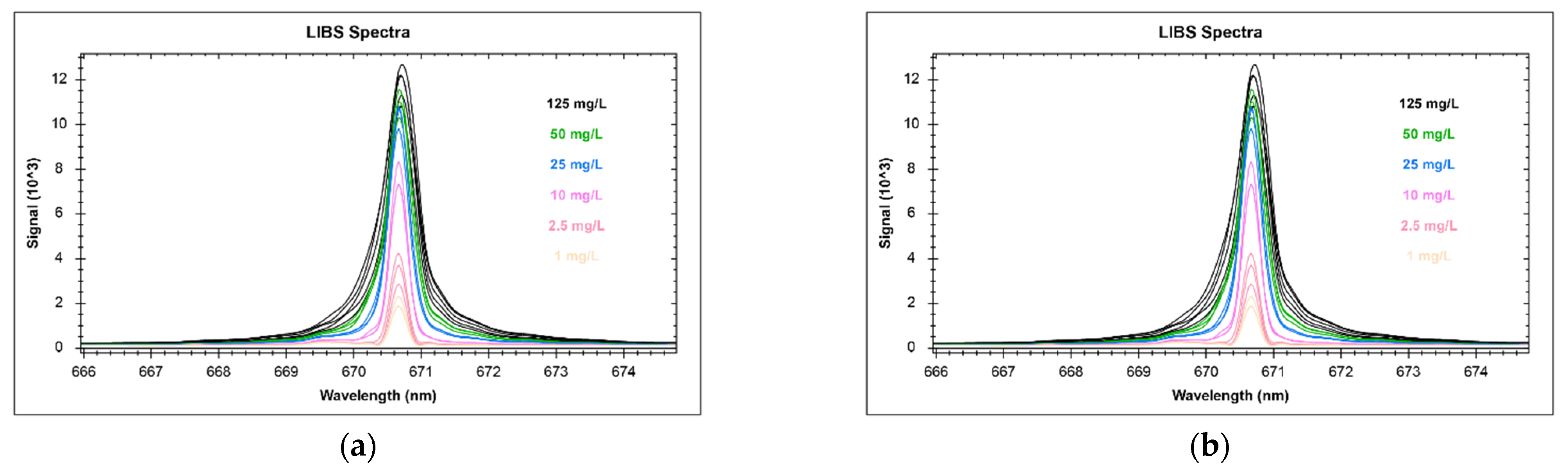
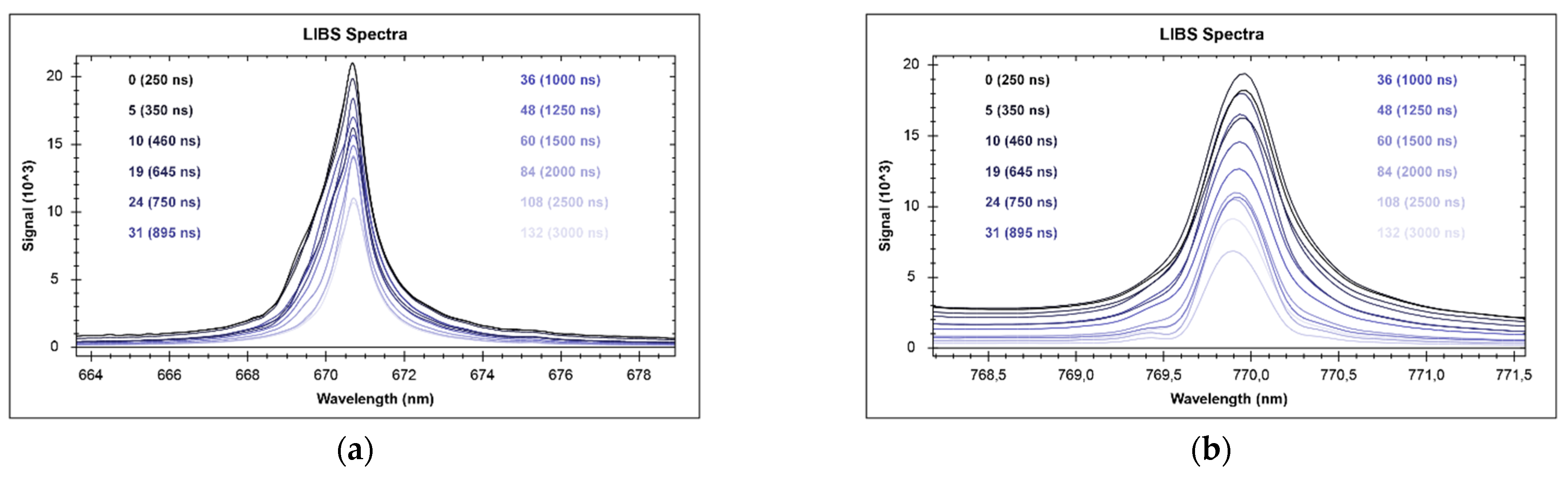
2.4. Calibration Settings
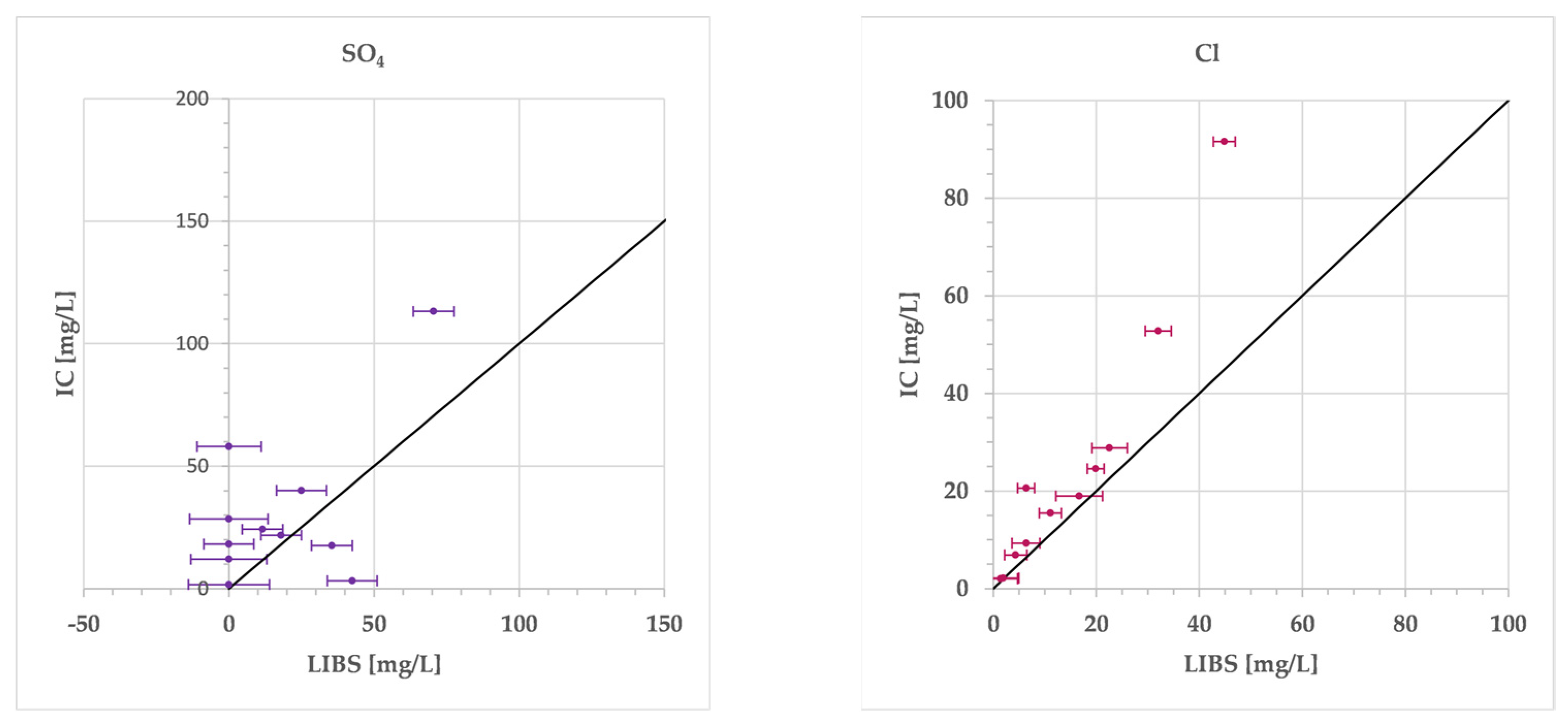
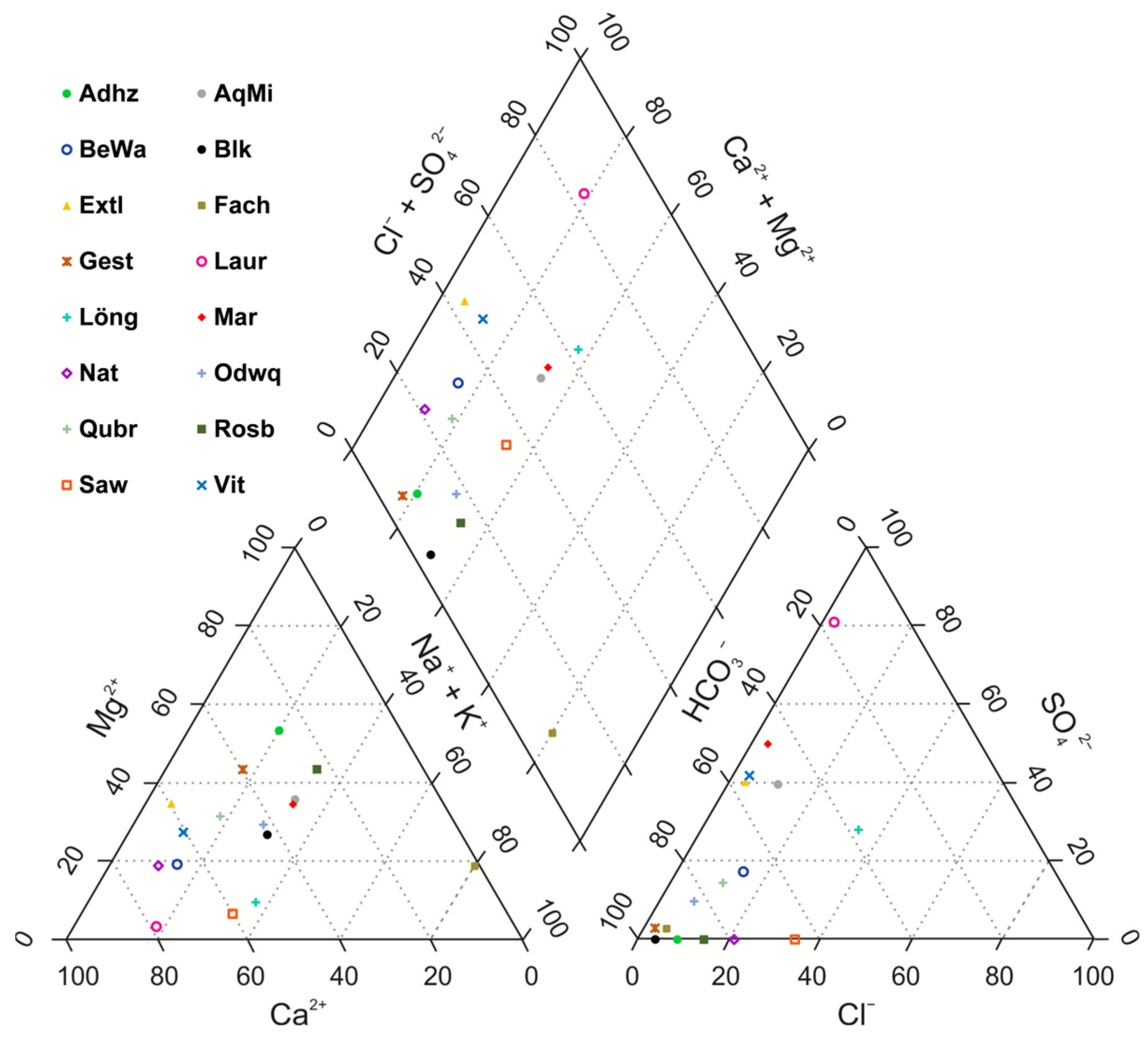
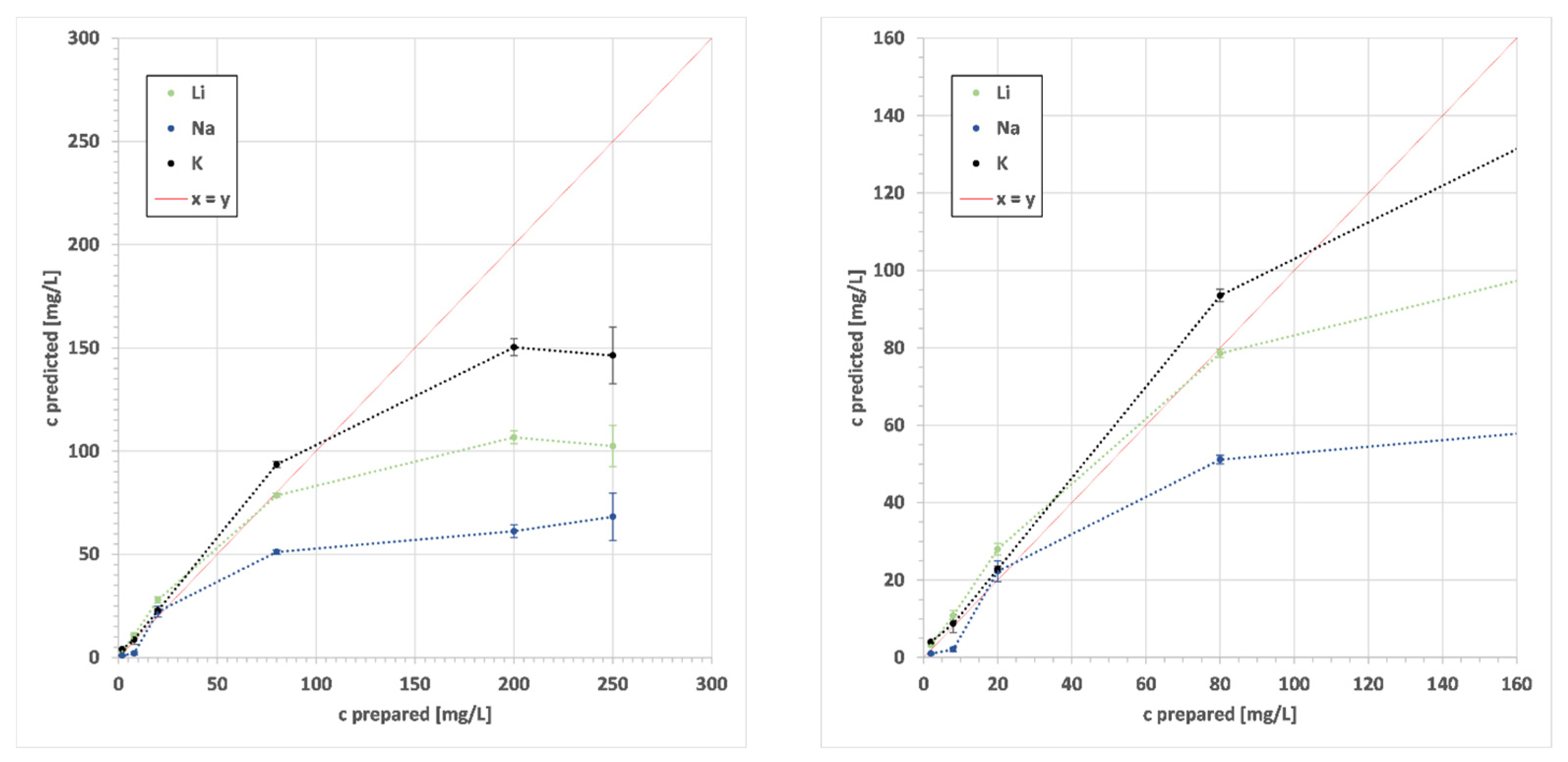
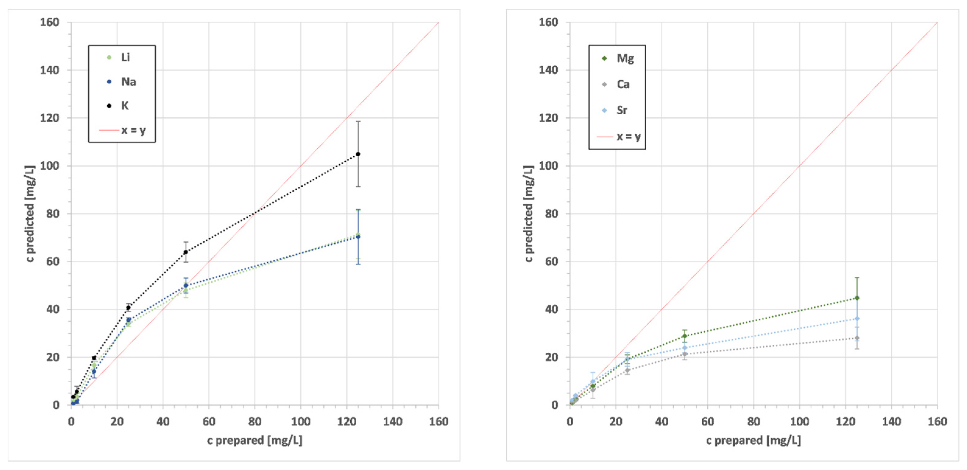
3. Results
4. Discussion
5. Conclusions
Author Contributions
Funding
Institutional Review Board Statement
Informed Consent Statement
Data Availability Statement
Acknowledgments
Conflicts of Interest
Appendix A

| Li | Na | Mg | K | Ca | Sr | SO4 | Cl | |
|---|---|---|---|---|---|---|---|---|
| THV I | 0.100 | 0.070 | 0.130 | 0.020 | 0.175 | 0.140 | 0.0002 | 0.0028 |
| THV II | 3.000 | 0.600 | 0.700 | 0.550 | 1.000 | 0.850 | ||
| mean b | 0.015 | 0.0141 | 0.0222 | 0.022 | 0.0093 | 0.0019 | 0.0003 | 0.0001 |
| Abbr. | Li | Na | Mg | K | Ca | Sr* | SO4 | Cl | Unit |
|---|---|---|---|---|---|---|---|---|---|
| RSD | 0.611 | 0.476 | 0.449 | 0.666 | 0.355 | 0.149 | 0.072 | % | |
| LoD | 0.028 | 0.019 | 0.059 | 0.053 | 0.098 | 0.0000214 | 0.218 | 0.075 | mg/L |
| SD | Li | Na | Mg | K | Ca | Sr | SO4 | Cl | Unit |
|---|---|---|---|---|---|---|---|---|---|
| Adhz | 0.06 | 4.21 | 4.86 | 0.73 | 3.08 | 0.23 | 13.51 | 4.56 | mg/L |
| BeWa | 0.06 | 1.89 | 0.51 | 0.54 | 2.62 | 0.00 | 7.00 | 2.14 | |
| Blk | 0.03 | 0.13 | 0.05 | 0.29 | 0.13 | 0.01 | 14.01 | 3.31 | |
| Gest | 0.06 | 4.23 | 4.94 | 0.97 | 5.28 | 0.08 | 7.00 | 1.65 | |
| Laur | 0.04 | 0.29 | 0.10 | 0.34 | 0.18 | 0.01 | 8.58 | 3.02 | |
| Löng | 0.05 | 3.21 | 0.21 | 0.20 | 3.23 | 0.01 | 8.58 | 3.44 | |
| Nat | 0.05 | 2.44 | 0.96 | 0.88 | 4.33 | 0.01 | 13.10 | 2.70 | |
| Odwq | 0.10 | 1.60 | 1.78 | 1.08 | 3.03 | 0.09 | 7.00 | 1.65 | |
| Rosb | 0.07 | 2.37 | 3.05 | 1.08 | 2.26 | 0.01 | 8.58 | 2.14 | |
| Saw | 0.15 | 9.52 | 0.74 | 0.71 | 4.24 | 0.03 | 11.07 | 2.53 | |
| Vit | 0.16 | 2.34 | 3.37 | 1.88 | 7.22 | 0.16 | 7.00 | 2.14 | |
| Median RSD | - | 25 | 17 | 29 | 11 | 22 | 39 | 26 | % |
References
- Zulkifli, S.N.; Rahim, H.A.; Lau, W.-J. Detection of Contaminants in Water Supply: A Review on State-of-the-Art Monitoring Technologies and Their Applications. Sens. Actuators B Chem. 2018, 255, 2657–2689. [Google Scholar] [CrossRef] [PubMed]
- Yaroshenko, I.; Kirsanov, D.; Marjanovic, M.; Lieberzeit, P.A.; Korostynska, O.; Mason, A.; Frau, I.; Legin, A. Real-Time Water Quality Monitoring with Chemical Sensors. Sensors 2020, 20, 3432. [Google Scholar] [CrossRef]
- Jan, F.; Min-Allah, N.; Düştegör, D. IoT Based Smart Water Quality Monitoring: Recent Techniques, Trends and Challenges for Domestic Applications. Water 2021, 13, 1729. [Google Scholar] [CrossRef]
- Lemière, B.; Uvarova, Y.A. New Developments in Field-Portable Geochemical Techniques and on-Site Technologies and Their Place in Mineral Exploration. Geochem. Explor. Environ. Anal. 2020, 20, 205–216. [Google Scholar] [CrossRef]
- Lemière, B.; Harmon, R.S. XRF and LIBS for Field Geology. In Portable Spectroscopy and Spectrometry; Crocombe, R., Leary, P., Kammrath, B., Eds.; Wiley: Hoboken, NJ, USA, 2021; pp. 455–497. ISBN 978-1-119-83557-8. [Google Scholar]
- Harmon, R.S.; Senesi, G.S. Laser-Induced Breakdown Spectroscopy—A Geochemical Tool for the 21st Century. Appl. Geochem. 2021, 128, 104929. [Google Scholar] [CrossRef]
- Schlatter, N.; Freutel, G.; Lottermoser, B.G. Evaluation of the Use of field-portable LIBS Analysers for on-site chemical Analysis in the Mineral Resources Sector. GeoResources 2022, 2, 32–38. [Google Scholar]
- Tiihonen, T.E.; Nissinen, T.J.; Turhanen, P.A.; Vepsäläinen, J.J.; Riikonen, J.; Lehto, V.-P. Real-Time on-Site Multielement Analysis of Environmental Waters with a Portable X-ray Fluorescence (PXRF) System. Anal. Chem. 2022, 94, 11739–11744. [Google Scholar] [CrossRef]
- Gałuszka, A.; Migaszewski, Z.M.; Namieśnik, J. Moving Your Laboratories to the Field—Advantages and Limitations of the Use of Field Portable Instruments in Environmental Sample Analysis. Environ. Res. 2015, 140, 593–603. [Google Scholar] [CrossRef]
- Cremers, D.A.; Radziemski, L.J.; Loree, T.R. Spectrochemical Analysis of Liquids Using the Laser Spark. Appl. Spectrosc. 1984, 38, 721–729. [Google Scholar] [CrossRef]
- Yueh, F.-Y.; Sharma, R.C.; Singh, J.P.; Zhang, H.; Spencer, W.A. Evaluation of the Potential of Laser-Induced Breakdown Spectroscopy for Detection of Trace Element in Liquid. J. Air Waste Manag. Assoc. 2002, 52, 1307–1315. [Google Scholar] [CrossRef]
- Zhao, F.; Chen, Z.; Zhang, F.; Li, R.; Zhou, J. Ultra-Sensitive Detection of Heavy Metal Ions in Tap Water by Laser-Induced Breakdown Spectroscopy with the Assistance of Electrical-Deposition. Anal. Methods 2010, 2, 408. [Google Scholar] [CrossRef]
- Lee, D.-H.; Han, S.-C.; Kim, T.-H.; Yun, J.-I. Highly Sensitive Analysis of Boron and Lithium in Aqueous Solution Using Dual-Pulse Laser-Induced Breakdown Spectroscopy. Anal. Chem. 2011, 83, 9456–9461. [Google Scholar] [CrossRef] [PubMed]
- Lee, Y.; Oh, S.-W.; Han, S.-H. Laser-Induced Breakdown Spectroscopy (LIBS) of Heavy Metal Ions at the Sub-Parts per Million Level in Water. Appl. Spectrosc. 2012, 66, 1385–1396. [Google Scholar] [CrossRef]
- Aguirre, M.A.; Legnaioli, S.; Almodóvar, F.; Hidalgo, M.; Palleschi, V.; Canals, A. Elemental Analysis by Surface-Enhanced Laser-Induced Breakdown Spectroscopy Combined with Liquid–Liquid Microextraction. Spectrochim. Acta Part B At. Spectrosc. 2013, 79–80, 88–93. [Google Scholar] [CrossRef]
- Cahoon, E.M.; Almirall, J.R. Quantitative Analysis of Liquids from Aerosols and Microdrops Using Laser Induced Breakdown Spectroscopy. Anal. Chem. 2012, 84, 2239–2244. [Google Scholar] [CrossRef]
- Bae, D.; Nam, S.-H.; Han, S.-H.; Yoo, J.; Lee, Y. Spreading a Water Droplet on the Laser-Patterned Silicon Wafer Substrate for Surface-Enhanced Laser-Induced Breakdown Spectroscopy. Spectrochim. Acta Part B At. Spectrosc. 2015, 113, 70–78. [Google Scholar] [CrossRef]
- Yang, X.; Yi, R.; Li, X.; Cui, Z.; Lu, Y.; Hao, Z.; Huang, J.; Zhou, Z.; Yao, G.; Huang, W. Spreading a Water Droplet through Filter Paper on the Metal Substrate for Surface-Enhanced Laser-Induced Breakdown Spectroscopy. Opt. Express 2018, 26, 30456. [Google Scholar] [CrossRef]
- Ma, S.; Tang, Y.; Ma, Y.; Chen, F.; Zhang, D.; Dong, D.; Wang, Z.; Guo, L. Stability and Accuracy Improvement of Elements in Water Using LIBS with Geometric Constraint Liquid-to-Solid Conversion. J. Anal. At. Spectrom. 2020, 35, 967–971. [Google Scholar] [CrossRef]
- Nakanishi, R.; Ohba, H.; Saeki, M.; Wakaida, I.; Tanabe-Yamagishi, R.; Ito, Y. Highly Sensitive Detection of Sodium in Aqueous Solutions Using Laser-Induced Breakdown Spectroscopy with Liquid Sheet Jets. Opt. Express 2021, 29, 5205. [Google Scholar] [CrossRef]
- Skrzeczanowski, W.; Długaszek, M. Application of Laser-Induced Breakdown Spectroscopy in the Quantitative Analysis of Elements—K, Na, Ca, and Mg in Liquid Solutions. Materials 2022, 15, 3736. [Google Scholar] [CrossRef] [PubMed]
- Tian, H.; Li, C.; Jiao, L.; Zhao, X.; Dong, D. Study on Rapid Detection Method of Water Heavy Metals by Laser-Induced Breakdown Spectroscopy Coupled with Liquid-Solid Conversion and Morphological Constraints. In Proceedings of the International Conference on Optoelectronic Materials and Devices (ICOMD 2021), Guangzhou, China, 10–12 December 2021; Lu, Y., Gu, Y., Chen, S., Eds.; SPIE: Guangzhou, China, 2022; p. 44. [Google Scholar]
- Zhang, Z.; Jia, W.; Shan, Q.; Hei, D.; Wang, Z.; Wang, Y.; Ling, Y. Determining Metal Elements in Liquid Samples Using Laser-Induced Breakdown Spectroscopy and Phase Conversion Technology. Anal. Methods 2022, 14, 147–155. [Google Scholar] [CrossRef] [PubMed]
- Bhatt, C.R.; Goueguel, C.L.; Jain, J.C.; McIntyre, D.L.; Singh, J.P. LIBS Application to Liquid Samples. In Laser-Induced Breakdown Spectroscopy; Elsevier: Amsterdam, The Netherlands, 2020; pp. 231–246. ISBN 978-0-12-818829-3. [Google Scholar]
- Schlatter, N.; Lottermoser, B.G. Quantitative Analysis of Li, Na, and K in Single Element Standard Solutions Using Portable Laser-Induced Breakdown Spectroscopy (pLIBS). Geochem. Explor. Environ. Anal. 2023, 23, geochem2023-019. [Google Scholar] [CrossRef]
- Birke, M.; Rauch, U.; Harazim, B.; Lorenz, H.; Glatte, W. Major and Trace Elements in German Bottled Water, Their Regional Distribution, and Accordance with National and International Standards. J. Geochem. Explor. 2010, 107, 245–271. [Google Scholar] [CrossRef]
- Birke, M.; Reimann, C.; Demetriades, A.; Rauch, U.; Lorenz, H.; Harazim, B.; Glatte, W. Determination of Major and Trace Elements in European Bottled Mineral Water—Analytical Methods. J. Geochem. Explor. 2010, 107, 217–226. [Google Scholar] [CrossRef]
- Reimann, C.; Birke, M. Geochemistry of European Bottled Water; Gebrüder Borntraeger: Stuttgart, Germany, 2010; ISBN 978-3-443-01067-6. [Google Scholar]
- Demetriades, A.; Reimann, C.; Birke, M. The Eurogeosurveys Geochemistry EGG Team European Ground Water Geochemistry Using Bottled Water as a Sampling Medium. In Clean Soil and Safe Water; Quercia, F.F., Vidojevic, D., Eds.; NATO Science for Peace and Security Series C: Environmental Security; Springer: Dordrecht, The Netherlands, 2012; pp. 115–139. ISBN 978-94-007-2239-2. [Google Scholar]
- Wise, M.A.; Harmon, R.S.; Curry, A.; Jennings, M.; Grimac, Z.; Khashchevskaya, D. Handheld LIBS for Li Exploration: An Example from the Carolina Tin-Spodumene Belt, USA. Minerals 2022, 12, 77. [Google Scholar] [CrossRef]
- Scott, J.R.; Effenberger, A.J.; Hatch, J.J. Influence of Atmospheric Pressure and Composition on LIBS. In Laser-Induced Breakdown Spectroscopy; Musazzi, S., Perini, U., Eds.; Springer Series in Optical Sciences; Springer: Berlin/Heidelberg, Germany, 2014; pp. 91–116. ISBN 978-3-642-45084-6. [Google Scholar]
- Schäffer, R.; Götz, E.; Schlatter, N.; Schubert, G.; Weinert, S.; Schmidt, S.; Kolb, U.; Sass, I. Fluid–Rock Interactions in Geothermal Reservoirs, Germany: Thermal Autoclave Experiments Using Sandstones and Natural Hydrothermal Brines. Aquat. Geochem. 2022, 28, 63–110. [Google Scholar] [CrossRef]
- DIN 38402-62:2014-12; German Standard Methods for the Examination of Water, Waste Water and Sludge—Part 62: Plausibility Check of Analytical Data by Performing an Ion Balance. Beuth Verlag GmbH: Berlin, Germany, 2014.
- Rossum, J.R. Conductance Method for Checking Accuracy of Water Analyses. Anal. Chem. 1949, 21, 631. [Google Scholar] [CrossRef]
- Legnaioli, S.; Botto, A.; Campanella, B.; Poggialini, F.; Raneri, S.; Palleschi, V. Univariate Linear Methods. In Chemometrics and Numerical Methods in LIBS; Palleschi, V., Ed.; Wiley: Hoboken, NJ, USA, 2022; pp. 259–276. ISBN 978-1-119-75961-4. [Google Scholar]
- Guezenoc, J.; Gallet-Budynek, A.; Bousquet, B. Critical Review and Advices on Spectral-Based Normalization Methods for LIBS Quantitative Analysis. Spectrochim. Acta Part B At. Spectrosc. 2019, 160, 105688. [Google Scholar] [CrossRef]
- IUPAC. Nomenclature, Symbols, Units and Their Usage in Spectrochemical Analysis—II. Data Interpretation. Pure Appl. Chem. 1976, 45, 99–103. [Google Scholar] [CrossRef]
- Schäffer, R.; Dietz, A. Standardized Schoeller Diagrams—A Matlab Plotting Tool. ESS Open Arch. 2022, 1–17. [Google Scholar] [CrossRef]
- Ma, S.; Tang, Y.; Zhang, S.; Ma, Y.; Sheng, Z.; Wang, Z.; Guo, L.; Yao, J.; Lu, Y. Chlorine and Sulfur Determination in Water Using Indirect Laser-Induced Breakdown Spectroscopy. Talanta 2020, 214, 120849. [Google Scholar] [CrossRef]
- Tang, Z.; Hao, Z.; Zhou, R.; Li, Q.; Liu, K.; Zhang, W.; Yan, J.; Wei, K.; Li, X. Sensitive Analysis of Fluorine and Chlorine Elements in Water Solution Using Laser-Induced Breakdown Spectroscopy Assisted with Molecular Synthesis. Talanta 2021, 224, 121784. [Google Scholar] [CrossRef] [PubMed]
- Poggialini, F.; Legnaioli, S.; Campanella, B.; Cocciaro, B.; Lorenzetti, G.; Raneri, S.; Palleschi, V. Calculating the Limits of Detection in Laser-Induced Breakdown Spectroscopy: Not as Easy as It Might Seem. Appl. Sci. 2023, 13, 3642. [Google Scholar] [CrossRef]
- Hark, R.R.; Harmon, R.S. Geochemical Fingerprinting Using LIBS. In Laser-Induced Breakdown Spectroscopy; Musazzi, S., Perini, U., Eds.; Springer Series in Optical Sciences; Springer: Berlin/Heidelberg, Germany, 2014; Volume 182, pp. 309–348. ISBN 978-3-642-45084-6. [Google Scholar]
- Samek, O.; Beddows, D.C.S.; Kaiser, J.; Kukhlevsky, S.V.; Liska, M.; Telle, H.H.; Whitehouse, A.J. Application of Laser-Induced Breakdown Spectroscopy to In Situ Analysis of Liquid Samples. Opt. Eng. 2000, 39, 2248. [Google Scholar] [CrossRef]
- Palleschi, V. Avoiding Misunderstanding Self-Absorption in Laser-Induced Breakdown Spectroscopy (LIBS) Analysis. Spectroscopy 2022, 37, 60–62. [Google Scholar] [CrossRef]
- Rao, A.P.; Jenkins, P.R.; Auxier, J.D.; Shattan, M.B.; Patnaik, A.K. Analytical Comparisons of Handheld LIBS and XRF Devices for Rapid Quantification of Gallium in a Plutonium Surrogate Matrix. J. Anal. At. Spectrom. 2022, 37, 1090–1098. [Google Scholar] [CrossRef]
- Tang, Y.; Ma, S.; Chu, Y.; Wu, T.; Ma, Y.; Hu, Z.; Guo, L.; Zeng, X.; Duan, J.; Lu, Y. Investigation of the Self-Absorption Effect Using Time-Resolved Laser-Induced Breakdown Spectroscopy. Opt. Express 2019, 27, 4261. [Google Scholar] [CrossRef] [PubMed]


| Abbr. | Name/Brand | Spring | Location | State | Country | Bottle | TDS (mg/L) | EC (µS/cm) |
|---|---|---|---|---|---|---|---|---|
| Adhz | Adelholzener | Adelholzener Alpen Quell | Bergen | BY | De | PET | 511 | 598 |
| AqMi | Aqua Mia | Geotaler | Löhne | NW | De | PET | 1284 | 1575 |
| BeWa | Bergische Waldquelle | Bergische Waldquelle | Haan | NW | De | PET | 159 | 257 |
| Blk | Blank sample | - | laboratory | - | - | HDPE | 1.3 | |
| Extl | Extaler-Mineralquell | Extaler-Mineralquell | Rinteln-Exten | NI | De | TP | 1603 | 1708 |
| Fach | Staatl. Fachingen | Staatl. Fachingen | Fachingen | RP | De | glass | 4306 | 2726 |
| Gest | Gerolsteiner Naturell | Naturell | Gerolstein | RP | De | PET | 807 | 878 |
| Laur | Lauretana | Lauretana | Graglia | 21 | It | PET | 17 | 20.5 |
| Löng | K-Classic | Quelle Löningen | Löningen | NI | De | PET | 162 | 275 |
| Mar | Marius-Quelle | Marius-Quelle | Sachsenheim | BW | De | PET | 2435 | 2650 |
| Nat | Naturalis still | Urstromquelle | Wolfhagen | HE | De | PET | 126 | 212 |
| Odwq | Odenwald-Quelle | Odenwald Quelle | Heppenheim | HE | De | PET | 760 | 727 |
| Qubr | Quellbrunn Werretaler | Werretaler | Löhne | NW | De | PET | 729 | 971 |
| Rosb | Rosbacher Naturell | Rosbacher Naturell | Rosbach v.d. Höhe | HE | De | PET | 1235 | 1363 |
| Saw | Sawell | Genussquelle 3 | Emsdetten | NW | De | PET | 377 | 589 |
| Vit | Vittel | Vittel Bonne Source | Vittel | 88 | Fr | PET | 490 | 444 |
| z | EoI | State | λ | LoD | Range | y | R2 | RMSE | S |
|---|---|---|---|---|---|---|---|---|---|
| nm | mg/L | mg/L | mg/L | mg/L | |||||
| 3 | Li | I | 497.1 | 0.006 | 0.1–2.5 | 28.133x − 0.3725 | 0.918 | 0.17 | 0.18 |
| I | 610.4 | 2.5–100 | 37.973x − 2.3069 | 0.995 | 6.65 | 6.71 | |||
| I | 670.8 | 100–1000 | 11.632x2.1134 | 0.954 | 202.18 | 204.19 | |||
| I | 812.9 | ||||||||
| 11 | Na | II | 330.2 | 0.014 | 0.1–2.5 | 45.219x + 0.0149 | 0.971 | 2.00 | 2.03 |
| I | 589.0 | 2.5–100 | 184.47x − 11.45 | 0.960 | 3.54 | 4.01 | |||
| I | 589.6 | 100–1000 | 8152.3x8.359 | 0.538 | 1131.01 | 1141.34 | |||
| I | 818.3 | ||||||||
| I | 819.5 | ||||||||
| 12 | Mg | II | 279.6 | 0.008 | 0.1–10 | 78.378x − 0.0589 | 0.979 | 0.00 | 0.00 |
| II | 279.8 | 10–100 | 173.46x − 14.439 | 0.973 | 6.83 | 6.93 | |||
| II | 280.3 | 100–1000 | - | - | - | - | |||
| I | 285.2 | ||||||||
| I | 293.6 | ||||||||
| I | 382.9 | ||||||||
| I | 383.2 | ||||||||
| I | 383.8 | ||||||||
| I | 516.7 | ||||||||
| I | 517.3 | ||||||||
| I | 518.4 | ||||||||
| 19 | K | I | 691.2 | 0.006 | 0.1–10 | 343.08 + 9.4034 | 0.987 | 0.49 | 0.49 |
| I | 693.9 | 10–160 | 292.55x + 9.7589 | 0.973 | 10.70 | 10.82 | |||
| I | 766.5 | 160–1000 | 62.902e1.6945x | 0.913 | 266.10 | 269.77 | |||
| I | 769.8 | ||||||||
| 20 | Ca | II | 315.9 | 0.021 | 0.1–2.5 | 23.014x − 0.0512 | 0.990 | 0.03 | 0.03 |
| II | 317.9 | 2.5–100 | 103.34x − 12.964 | 0.893 | 3.79 | 3.82 | |||
| II | 318.1 | 100–1000 | −527.31x2 + 2456.7x − 1766.7 | 0.889 | 155.42 | 157.59 | |||
| II | 370.6 | ||||||||
| II | 393.3 | ||||||||
| II | 396.8 | ||||||||
| I | 422.6 | ||||||||
| I | 430.2 | ||||||||
| I | 430.8 | ||||||||
| I | 443.5 | ||||||||
| I | 445.5 | ||||||||
| I | 526.5 | ||||||||
| I | 527.0 | ||||||||
| I | 558.9 | ||||||||
| 30 | Zn | II | 202.6 | 0.0005 | 0.1–2.5 | 621.9x − 0.1649 | 0.988 | 0.07 | 0.07 |
| I | 213.9 | 2.5–50 | 544.01 − 0.4883 | 0.998 | 1.38 | 1.40 | |||
| I | 334.5 | 50–1000 | 2449.2x2 + 1115.7x − 94.322 | 0.989 | 102.14 | 103.02 | |||
| I | 468.0 | ||||||||
| I | 481.1 | ||||||||
| I | 636.2 | ||||||||
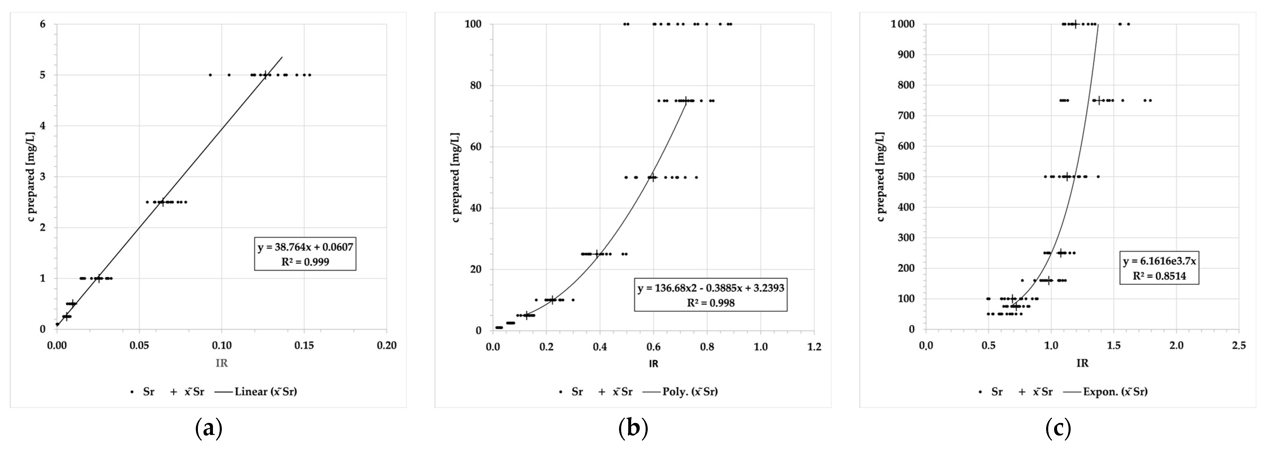
| 38 | Sr | II | 215.3 | 0.0008 | 0.1–5 | 38.764x + 0.0607 | 0.999 | 0.14 | 0.14 |
| II | 216.6 | 5–75 | 136.68x2 − 0.3885x + 3.2393 | 0.998 | 7.64 | 7.74 | |||
| II | 338.1 | 75–1000 | 6.1616e3.7x | 0.851 | 4708.79 | 4754.73 | |||
| II | 407.7 | ||||||||
| II | 416.2 | ||||||||
| II | 421.6 | ||||||||
| II | 430.6 | ||||||||
| I | 460.7 | ||||||||
| I | 496.2 | ||||||||
| I | 525.7 | ||||||||
| I | 548.1 | ||||||||
| 7 | N | II | 567.6 | 0.0017 | 0.5–160 | 2014.3x | 0.853 | 105.13 | 105.97 |
| II | 568.6 | 160–1000 | 100.07e7.0029x | 0.872 | 195.30 | 197.96 | |||
| 16 | S | I | 921.2 | 0.0002 | 0.5–160 | 175098x + 106.97 | 0.647 | 93.42 | 94.12 |
| I | 922.8 | 160–1000 | 109.42e2043.1x | 0.829 | 621.23 | 629.69 | |||
| I | 923.7 | ||||||||
| 17 | Cl | I | 833.3 | 0.0004 | 0.5–160 | 33588x | 0.976 | 97.18 | 98.04 |
| I | 837.6 | 160–1000 | 18.869e561.95x | 0.912 | 1113.22 | 1126.09 | |||
| I | 857.5 | ||||||||
| I | 858.6 | ||||||||
| I | 894.8 | ||||||||
| 13 | Al * | I | 236.7 | ||||||
| I | 237.3 | ||||||||
| I | 308.2 | ||||||||
| I | 394.4 | ||||||||
| I | 396.1 |
| Abbr. | Li | Na | Mg | K | Ca | Sr | SO4 | Cl | Unit | IB | EC | ||
|---|---|---|---|---|---|---|---|---|---|---|---|---|---|
| eq-% | µS/cm | ||||||||||||
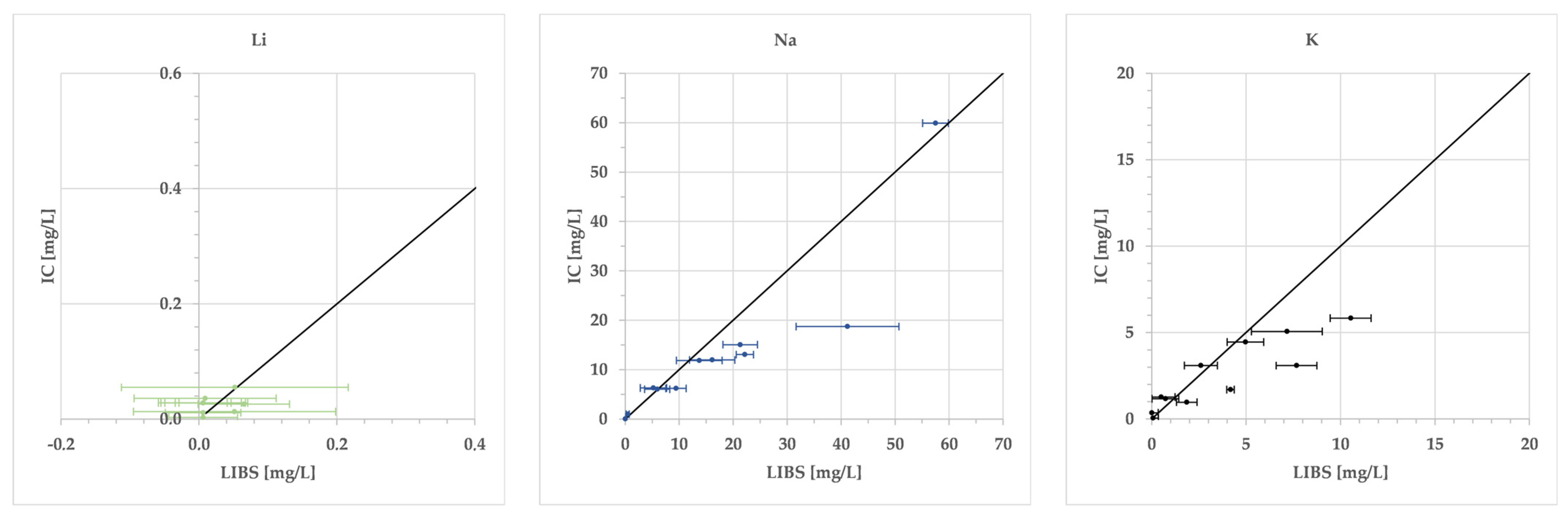
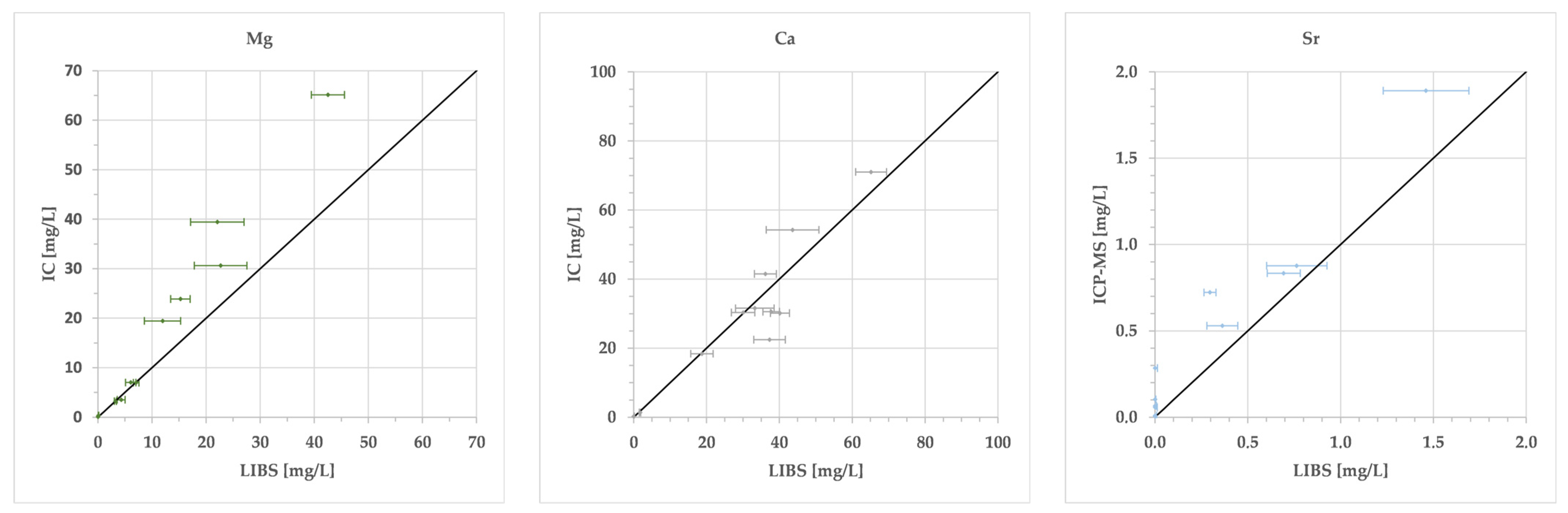
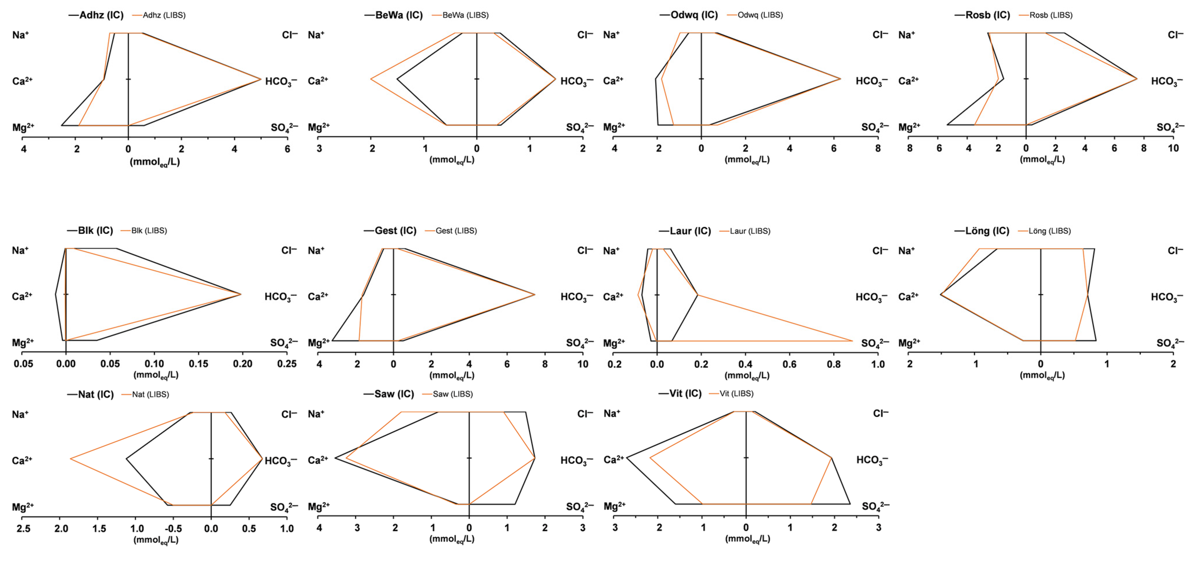
| Adhz | lab | <LoD | 11.95 | 30.63 | 1.26 | 18.40 | 1.891 | 28.46 | 18.95 | mg/L | −41.3 | 496 | lab |
| pLIBS | <LoD | 16.11 | 22.69 | 0.32 | 18.74 | 1.460 | <LoD | 16.71 | mg/L | −44.9 | 434 | pLIBS | |
| dev | 0.022 | 4.16 | 7.94 | 0.95 | 0.34 | 0.431 | 28.46 | 2.24 | mg/L | 598 | meas | ||
| r-dev | 78.6 | 34.8 | 25.9 | 74.8 | 1.9 | 22.8 | 100 | 11.8 | % | −3.7 | −164 | dev | |
| BeWa | lab | <LoD | 6.19 | 6.96 | 0.97 | 30.16 | 0.103 | 21.81 | 15.46 | mg/L | −0.7 | 252 | lab |
| pLIBS | <LoD | 9.41 | 7.06 | 1.86 | 40.15 | <LoD | 17.98 | 11.08 | mg/L | 30.2 | 277 | pLIBS | |
| dev | 0.022 | 3.21 | 0.10 | 0.88 | 9.99 | 0.1022 | 3.83 | 4.37 | mg/L | 257 | meas | ||
| r-dev | 78.6 | 51.9 | 1.4 | 91.1 | 33.1 | 99.2 | 17.5 | 28.3 | % | 30.9 | 20 | dev | |
| Blk | lab | <LoD | <LoD | <LoD | <LoD | 0.24 | 0.004 | 1.68 | 2.01 | mg/L | −171.2 | 17 | lab |
| pLIBS | <LoD | <LoD | <LoD | 0.01 | <LoD | <LoD | <LoD | 0.28 | mg/L | −193.6 | 9 | pLIBS | |
| dev | 0.022 | 0.005 | 0.051 | 0.047 | 0.077 | 0.003 | 1.68 | 1.73 | mg/L | 1 | meas | ||
| r-dev | 78.6 | 26.3 | 86.4 | 88.7 | 78.6 | 79.4 | 100 | 86.2 | % | −22.4 | 8 | dev | |
| Gest | lab | <LoD | 11.86 | 39.42 | 4.45 | 31.57 | 0.529 | 24.23 | 20.61 | mg/L | −45.8 | 684 | lab |
| pLIBS | <LoD | 13.71 | 22.08 | 4.96 | 33.25 | 0.363 | 10.98 | 6.36 | mg/L | −61.8 | 573 | pLIBS | |
| dev | 0.022 | 1.85 | 17.34 | 0.52 | 1.69 | 0.166 | 13.25 | 14.25 | mg/L | 878 | meas | ||
| r-dev | 78.6 | 15.6 | 44.0 | 11.6 | 5.3 | 31.4 | 54.7 | 69.2 | % | −15.9 | −305 | dev | |
| Laur | lab | <LoD | 0.97 | 0.34 | 0.36 | 1.38 | 0.010 | 3.21 | 2.13 | mg/L | −73.2 | 26 | lab |
| pLIBS | <LoD | 0.46 | 0.04 | 0.01 | 1.74 | < LoD | 42.50 | 0.95 | mg/L | −163.0 | 81 | pLIBS | |
| dev | 0.022 | 0.51 | 0.29 | 0.35 | 0.36 | 0.009 | 39.29 | 1.18 | mg/L | 21 | meas | ||
| r-dev | 78.6 | 52.1 | 86.9 | 98.3 | 26.2 | 91.8 | 1225 | 55.3 | % | −89.9 | 60 | dev | |
| Löng | lab | <LoD | 15.05 | 3.23 | 1.70 | 30.33 | 0.066 | 40.08 | 28.79 | mg/L | 4.8 | 281 | lab |
| pLIBS | <LoD | 21.31 | 3.23 | 4.17 | 30.05 | 0.001 | 24.99 | 22.56 | mg/L | 29.1 | 278 | pLIBS | |
| dev | 0.022 | 6.25 | 0.00 | 2.47 | 0.28 | 0.065 | 15.09 | 6.22 | mg/L | 275 | meas | ||
| r-dev | 78.6 | 41.5 | 0.0 | 145 | 0.9 | 98.8 | 37.6 | 21.6 | % | 24.3 | 3 | dev | |
| Nat | lab | <LoD | 6.28 | 7.01 | 3.09 | 22.48 | 0.057 | 12.02 | 9.29 | mg/L | 46.8 | 177 | lab |
| pLIBS | <LoD | 5.21 | 6.05 | 2.60 | 37.28 | 0.001 | 0.00 | 6.36 | mg/L | 98.8 | 182 | pLIBS | |
| dev | 0.022 | 1.07 | 0.96 | 0.49 | 14.80 | 0.056 | 12.02 | 2.94 | mg/L | 212 | meas | ||
| r-dev | 78.6 | 17.0 | 13.7 | 15.8 | 65.9 | 98.6 | 100 | 31.6 | % | 52.1 | −30 | dev | |
| Odwq | lab | 0.036 | 13.04 | 23.87 | 5.83 | 41.52 | 0.834 | 17.56 | 24.54 | mg/L | −42.7 | 592 | lab |
| pLIBS | <LoD | 22.15 | 15.25 | 10.54 | 36.16 | 0.694 | 35.49 | 19.86 | mg/L | −57.1 | 602 | pLIBS | |
| dev | 0.030 | 9.11 | 8.62 | 4.71 | 5.37 | 0.140 | 17.94 | 4.68 | mg/L | 727 | meas | ||
| r-dev | 83.3 | 69.9 | 36.1 | 80.7 | 12.9 | 16.8 | 102 | 19.1 | % | −14.4 | −125 | dev | |
| Rosb | lab | <LoD | 59.91 | 65.13 | 3.09 | 30.59 | 0.284 | 18.15 | 91.57 | mg/L | −9.2 | 1016 | lab |
| pLIBS | 0.057 | 57.49 | 42.53 | 7.67 | 37.75 | 0.001 | 0.0002 | 44.85 | mg/L | −16.4 | 876 | pLIBS | |
| dev | 0.029 | 2.42 | 22.60 | 4.58 | 7.17 | 0.284 | 18.15 | 46.72 | mg/L | 1363 | meas | ||
| r-dev | 103 | 4.0 | 34.7 | 148 | 23.4 | 100 | 100 | 51.0 | % | −7.3 | −487 | dev | |
| Saw | lab | <LoD | 18.73 | 3.52 | 1.17 | 71.03 | 0.722 | 58.00 | 52.78 | mg/L | 3.7 | 524 | lab |
| pLIBS | <LoD | 41.18 | 4.29 | 0.62 | 65.17 | 0.296 | 0.0002 | 32.02 | mg/L | 60.5 | 439 | pLIBS | |
| dev | 0.022 | 22.45 | 0.78 | 0.55 | 5.86 | 0.427 | 58.00 | 20.76 | mg/L | 589 | meas | ||
| r-dev | 78.6 | 120 | 22.1 | 47.1 | 8.2 | 59.0 | 100 | 39.3 | % | 56.8 | −150 | dev | |
| Vit | lab | 0.055 | 6.02 | 19.45 | 5.07 | 54.26 | 0.877 | 113.17 | 6.87 | mg/L | 5.0 | 511 | lab |
| pLIBS | <LoD | 5.93 | 11.94 | 7.16 | 43.63 | 0.764 | 70.51 | 4.33 | mg/L | 1.5 | 390 | pLIBS | |
| dev | 0.049 | 0.09 | 7.51 | 2.09 | 10.63 | 0.113 | 42.65 | 2.54 | mg/L | 444 | meas | ||
| r-dev | 89.1 | 1.5 | 38.6 | 41.4 | 19.6 | 12.9 | 37.7 | 37.0 | % | −3.6 | −54 | dev | |
| Median r-dev | 78.6 | 34.8 | 34.7 | 80.7 | 19.6 | 79.4 | 100.0 | 37.0 | % | ||||
Disclaimer/Publisher’s Note: The statements, opinions and data contained in all publications are solely those of the individual author(s) and contributor(s) and not of MDPI and/or the editor(s). MDPI and/or the editor(s) disclaim responsibility for any injury to people or property resulting from any ideas, methods, instructions or products referred to in the content. |
© 2023 by the authors. Licensee MDPI, Basel, Switzerland. This article is an open access article distributed under the terms and conditions of the Creative Commons Attribution (CC BY) license (https://creativecommons.org/licenses/by/4.0/).
Share and Cite
Schlatter, N.; Lottermoser, B.G.; Illgner, S.; Schmidt, S. Utilising Portable Laser-Induced Breakdown Spectroscopy for Quantitative Inorganic Water Testing. Chemosensors 2023, 11, 479. https://doi.org/10.3390/chemosensors11090479
Schlatter N, Lottermoser BG, Illgner S, Schmidt S. Utilising Portable Laser-Induced Breakdown Spectroscopy for Quantitative Inorganic Water Testing. Chemosensors. 2023; 11(9):479. https://doi.org/10.3390/chemosensors11090479
Chicago/Turabian StyleSchlatter, Nils, Bernd G. Lottermoser, Simon Illgner, and Stefanie Schmidt. 2023. "Utilising Portable Laser-Induced Breakdown Spectroscopy for Quantitative Inorganic Water Testing" Chemosensors 11, no. 9: 479. https://doi.org/10.3390/chemosensors11090479
APA StyleSchlatter, N., Lottermoser, B. G., Illgner, S., & Schmidt, S. (2023). Utilising Portable Laser-Induced Breakdown Spectroscopy for Quantitative Inorganic Water Testing. Chemosensors, 11(9), 479. https://doi.org/10.3390/chemosensors11090479