A Qualitative and Quantitative Analysis Strategy for Continuous Turbulent Gas Mixture Monitoring

Abstract

Electronic noses are one of the predominant technological choices for gas mixture detection, but their application in real-world atmospheric environments still leaves several issues to be resolved. The key bottleneck is the effect of turbulence caused by the diffusion of gases in the atmosphere on the quantitative and qualitative analytical performance of the electronic nose. In light of this, this paper presents a quantitative and qualitative analysis strategy for gas mixture monitoring. This strategy adopts baseline manipulation of the raw sensor data to reduce drift interference, and then performs feature extraction on the multidimensional response signals of the MOS gas sensor array using principal component analysis (PCA). In order to improve gas mixture recognition accuracy, the whale optimization algorithm (WOA) is used to optimize the network structure of the long short-term memory (LSTM) model for turbulent gas mixture composition recognition. The least squares support vector machine (LSSVM) algorithm is adopted to implement turbulent gas mixture concentration prediction. This paper focuses on two aspects of hyper-parameter optimization for the development of an LSSVM with particle swarm optimization (PSO) and for improved training sample selection for the LSSVM which should subsequently increase the accuracy of concentration estimation. The effectiveness of the proposed strategy is evaluated with a dataset from a chemical sensor array exposed to turbulent gas mixtures. Experimental results revealed that the proposed strategy for turbulent gas mixtures has satisfactory outcomes for both qualitative gas composition recognition and quantitative gas concentration prediction.

1. Introduction

The human living environment is surrounded by a variety of gases. Although the presence of these gases can easily be neglected, the gases in the environment frequently contain a lot of important information that can be used by people. Currently, there are many ways to achieve gas detection, among which artificial olfactory systems [1], also known as electronic noses (e-noses), offer a promising low-cost, simple structured, portable solution for gas detection and have become one of the hot spots for academic research in this field. E-noses have shown prospective applications in food quality monitoring, public safety, assisted medical diagnosis, atmospheric environmental monitoring, flammable and explosive gas detection, and space capsule environmental monitoring [2,3,4,5,6,7,8]. Gas sensor arrays and pattern recognition methods are the core components of the e-nose [9]. Limited by the selectivity and sensitivity of existing commercial gas sensors, the performance of the pattern recognition method determines the results of the qualitative and quantitative analysis of the gas by the e-nose to a large extent [10]. In recent years, many scholars have used many different pattern recognition methods to improve the accuracy of e-noses for gas detection and have achieved considerable results. Fan et al. proposed a qualitative and quantitative multi-component analysis strategy for gas mixtures using a gas sensor array [11]. The analysis strategy used principal component analysis (PCA) combined with a random forest (RF) as a qualitative identification method for mixed gases, and support vector regression (SVR) optimized by the particle swarm optimization (PSO) method was adopted for quantitative analysis. Laref et al. discussed the positive effect of hyper-parameter optimization of the SVR algorithm on the accuracy of electronic nose gas concentration analysis [12]. Gamboa et al. investigated three different deep learning models and compared them with support vector machines (SVM) in terms of their effectiveness regarding fast gas detection [13]. The experimental results showed that SVM obtained the highest accuracy and the least training time. Chen et al. proposed a concentration estimation method of mixed volatile organic compounds (VOCs) for gas sensor arrays based on use of a back propagation neural network (BPNN) coupled with decision tree learning [14]. Bakiler et al. presented a mixed gas detection method, which uses LSTM to extract features from the steady-state response signals of the gas sensor array and then adopts SVM to achieve gas identification and concentration estimation [15]. Chu et al. utilized a genetic algorithm (GA) to optimize the BPNN model to achieve accurate identification of multiple gas mixtures with different concentrations [16]. It can be seen from the above research that the research core of gas detection using an electronic nose mainly focuses on selecting appropriate pattern recognition methods to solve the classification and regression problems.

Although the above research has been effective in achieving mixture composition identification and concentration prediction to some extent, the following two main issues still cannot be ignored. Firstly, most of the existing methods ignore the impact of turbulent gas diffusion on the detection accuracy of gas mixtures in real atmospheric environments. Because the datasets used for training gas detection models are obtained from laboratories with strictly controlled experimental parameters and mostly under static experimental conditions, the developed models are unsuitable for dynamic turbulent gas mixture detection [17]. In practice, the diffusion of gases in the atmospheric environment is indefinite and dynamic, and the direction and concentration of diffusion are constantly changing, which is the bottleneck problem that restricts the application of e-noses to the real-world atmospheric environment. Secondly, the impact of training sample selection strategy on the performance of the mixed gas detection model cannot be ignored. Previous investigations have focused more on model parameter optimization in order to improve detection accuracy. Fonollosa et al. experimentally verified that the selection of samples with different concentration levels in the training sample set precisely determines the measurement range and accuracy of the detection model [18]. The complexity of mixed gas detection is significantly increased by the fact that various gaseous analytes undergo diffusion, turbulence, and advection in the atmospheric environment, and by the fact that most chemical gas sensors are susceptible to environmental changes. Therefore, the design of a qualitative and quantitative analysis strategy applicable to turbulent gas mixtures is of great importance when seeking to improve the performance of e-noses in realistic, uncontrolled natural scenarios.

At present, only a few studies have attempted to investigate theoretical and experimental approaches for the composition detection of turbulent gas mixtures [16,17,18,19,20]. In this paper, a qualitative and quantitative analysis strategy for turbulent gas mixture monitoring is proposed and an experimental study of different training sample selection strategies is conducted in order to achieve more effective detection. Firstly, baseline correction of the gas sensor array response signal is performed using the fractional difference method to reduce the drift effect under long-term monitoring conditions, and the relative resistance value method is then employed to further highlight the signal features. Secondly, feature extraction of the response signal of the sensor array is realized by principal component analysis (PCA). After that, the qualitative identification of turbulent gas mixtures is solved by using the capability of long short-term memory (LSTM) neural networks to process unstable time series data with fixed components. LSTM has advantages in time series modelling and has a long-time memory function, which is simple to implement and solves the gradient disappearance and gradient explosion problems that exist in the long series training process. LSTM has good performance when processing multivariate signals from MOS gas sensor arrays. In order to improve the gas recognition accuracy of the LSTM model, this paper uses the whale optimization algorithm (WOA) to balance the ability to globally search and locally search effectively and optimizes the learning rate and the number of hidden neural layer units of the LSTM model to further construct the WOA-LSTM model for gas recognition. As for the quantitative estimation of turbulent gas mixture concentration, the least squares support vector machine (LSSVM) is used as the concentration prediction model in this paper. The LSSVM introduces two important parameters (kernel function parameter, regularization parameter), where the kernel parameter has a direct impact on the complexity of the distribution of low-dimensional sample data in the mapping space and the regularization parameter is related to the fit of the model to the training samples and the ability of the model to generalize. As a result, the LSSVM shows many unique advantages in small sample, non-linear, and high-dimensional pattern recognition problems, modelling with advantages such as good prediction accuracy, fast modelling, and strong learning ability. In order to solve the problem of selecting the parameters of the LSSVM kernel function, this paper optimizes its parameters by using the particle swarm optimization (PSO) algorithm to further improve gas concentration estimation accuracy. Finally, the performance of the proposed qualitative and quantitative analysis method of turbulent gas mixtures is experimentally verified using different training sample selection strategies.

The rest of this paper is organized as follows. The relevant theoretical approaches utilized in this paper are presented in Section 2. Section 3 describes the proposed qualitative and quantitative analysis strategy for turbulent gas mixtures. Section 4 illustrates the performance of the proposed method through experiments. Section 5 summarizes the conclusions drawn from the results.

2. Methods

2.1. Long Short-Term Memory

The long short-term memory (LSTM) network was proposed by Hochreiter in 1997 as an improved recurrent neural network (RNN) for time series learning tasks [21]. Compared to the traditional RNN model, LSTM introduces a new structure cell that helps solve the long-term dependencies of time series and is suitable for learning classification from experience. The basic principle of LSTM is described as follows.

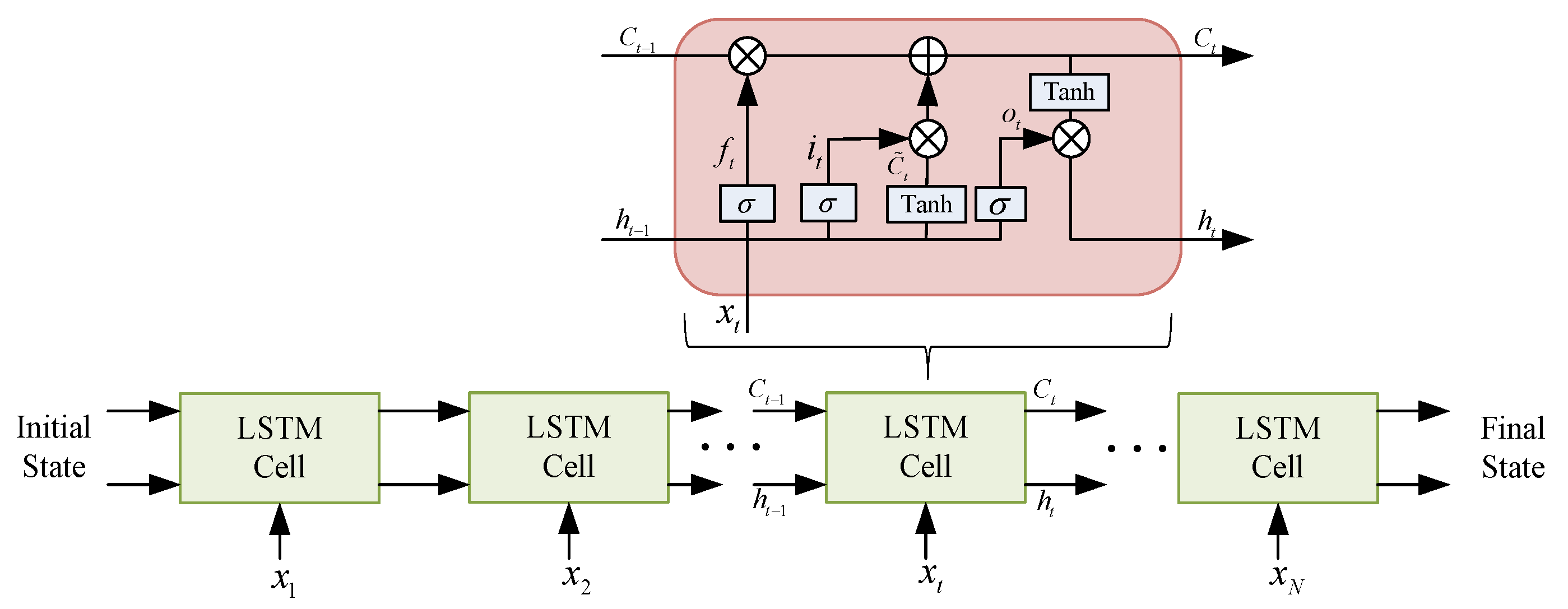
The structure of a standard LSTM network is shown in Figure 1. The LSTM cell consists of three gates, namely an input gate, a forget gate, and an output gate. The gates control the discarding or adding of information for forgetting or remembering functions.

The input gate determines which new information from $x_t$ can be stored in the cell state $C_t$.

$$i_t=\sigma (W_i\cdot [h_{t-1},x_t]+b_i)$$

(1)

$${\tilde{C}}_t=\tanh (W_C\cdot [h_{t-1},x_t]+b_C)$$

(2)

where $\sigma (\cdot )$ is a sigmoid function that converts the variable to a value between $[0,1]$; $\tanh (\cdot )$ is a hyperbolic tangent function which outputs a value between $[-1,1]$; $x_t$ denotes the input value at moment t; $h_t$ denotes the hidden state at moment t; $W$ denotes the weights; and $b$ denotes the bias.

The forget gate decides which information is discarded from the cell state. $f_t$ determines how much of the previous cell state $C_{t-1}$ is retained to the current cell state $C_t$.

$$f_t=\sigma (W_f\cdot [h_{t-1},x_t]+b_f)$$

(3)

$$C_t=f_t\ast C_{t-1}+i_t\ast {\tilde{C}}_t$$

(4)

The output gate is used to control how much information is filtered out in the new state $C_t$.

$$o_t=f(W_o\cdot [h_{t-1},x_t]+b_o)$$

(5)

$$h_t=o_t\ast \tanh (C_t)$$

(6)

2.2. Least Squares Support Vector Machine

The least squares support vector machine (LSSVM) is an extension of the standard SVM that is more suitable for solving high-dimensional learning problems; the machine has faster solving speed and excellent generalization capabilities [22,23].

Given a set of samples, ${\{x_i,y_i\}}_{i=1}^N$, $x_i\in {ℝ}^n$ and $y_i\in (-1,1)$, the optimization problem of the LSSVM is formulated in the following form,

$$\begin{array}{l}\underset{w,b,e}{\min }J(w,e_i)=\frac{1}{2}\Vert w\Vert +\frac{1}{2}\gamma {\displaystyle \sum _{i=1}^N{e}_i^2}\\ s.t. y_i=w^T\phi (x_i)+b+e_i,i=1,2,\dots ,N\end{array}$$

(7)

where $w$ is the weight vector, $\gamma$ is penalty coefficient, and $e_i$ is the random error. $\phi (\cdot )$ is the non-linear mapping function that maps $x_i$ into a higher dimensional feature space. $b$ is a bias term.

A Lagrangian function is built to solve the LSSVM as follows.

$$L(w,b,e_i,{\alpha }_i)=J(w,e_i)-{\displaystyle \sum _{i=1}^N{\alpha }_i(w\phi (x_i)+b+e_i-y_i)}$$

(8)

where ${\alpha }_i$ is the Lagrangian multiplier. Equation (8) is solved as described below,

$$\{\begin{array}{c}\frac{\partial L}{\partial w}=0\Rightarrow w={\displaystyle \sum _{i=1}^N{\alpha }_i\phi (x_i)}\\ \frac{\partial L}{\partial b}=0\Rightarrow {\displaystyle \sum _{i=1}^N{\alpha }_i=0}\\ \frac{\partial L}{\partial e_i}=0\Rightarrow {\alpha }_i=C{e}_i\\ \frac{\partial L}{\partial {\alpha }_i}=0\Rightarrow w\phi (x_i)+b+e_i-y_i=0\end{array}$$

(9)

A linear system for classification and regression can be obtained and its solution is found by solving the system of linear equations expressed in matrix form as follows:

$$\left[\begin{array}{cc}0& I^T\\ I& Z{Z}^T+{\gamma }^{-1}I\end{array}\right]\left[\begin{array}{c}b\\ a\end{array}\right]=\left[\begin{array}{c}0\\ y\end{array}\right]$$

(10)

where $I={[1,1,\cdots ,1]}^T$, $Z={[\phi (x_1),\phi (x_2),\cdots ,\phi (x_N)]}^T$, $a={[a_1,a_2,\cdots ,a_N]}^T$, $y={[y_1,y_2,\cdots ,y_N]}^T$.

The regression function of the LSSVM is described as follows:

$$f(x)={\displaystyle \sum _{i=1}^N{a}_i}K(x_i,x)+b$$

(11)

where the kernel function is given by $K(x_i,x)=\phi (x_i)\phi (x)$ and meets Mercer criteria. The Gaussian kernel is a widely used kernel function that is defined as

$$k(x,x_j)=\exp \left(-\frac{{\Vert x-x_j\Vert }^2}{2{\sigma }^2}\right)$$

(12)

where $\sigma$ is the width of the Gaussian kernel that influences the performance of the regression model. The penalty coefficient $\gamma$ is another critical parameter that affects the performance of the regression model.

2.3. WOA-LSTM

The WOA optimization algorithm mainly imitates the behavior of humpback whales surrounding prey, bubble-net attack, and searching for prey, and obtains the global optimal solution in the search space [24]. Compared to other optimization algorithms, the WOA has better optimization ability, faster convergence speed, higher calculation accuracy, and stronger robustness. The basic principle of the WOA algorithm is as follows.

• Encircling prey

In D-dimensional space, the position of each whale is

$$X=(x_1,x_2,\cdots ,x_D)$$

(13)

Humpback whales can sense the location of their prey and gradually surround them. As the location of the optimal solution in the search space is usually unpredictable, the WOA modeling process assumes that the current optimal candidate solution is the target prey. Once the best search agent has been determined, the other search agents will update their positions to approximate the current best search agent. This behavior is represented by the following equations.

$$\overrightarrow{D}=|\overrightarrow{C}\times {\overrightarrow{X}}^{*}(n)-\overrightarrow{X}(n)|$$

(14)

$$\overrightarrow{X}(n+1)={\overrightarrow{X}}^{*}(n)-\overrightarrow{A}\times \overrightarrow{D}$$

(15)

where n indicates the current iteration number, $\overrightarrow{A}$ and $\overrightarrow{C}$ are coefficient vectors, ${\overrightarrow{X}}^{*}(n)$ is the position vector of the optimal solution, $\overrightarrow{X}(n)$ is the position vector of the current solution, and $|·|$ denotes the absolute value operation. ${\overrightarrow{X}}^{*}(n)$ is updated each time a better solution appears during each interaction.

The coefficient vectors $\overrightarrow{A}$ and $\overrightarrow{C}$ are obtained by Equations (16) and (17).

$$\overrightarrow{A}=2\overrightarrow{a}\cdot \overrightarrow{r}-\overrightarrow{a}$$

(16)

$$\overrightarrow{C}=2\overrightarrow{r}$$

(17)

where $\overrightarrow{r}$ is a random number in $[0,1]$ and $\overrightarrow{a}$ is a control parameter that decreases linearly from 2 to 0 as the number of iterations increases.

2

Bubble-net attacking method

During the process of encircling prey, whales update their position according to two mechanisms: the shrinking encirclement mechanism and the spiral position updating mechanism.

• Shrinking encirclement mechanism

Shrinking encirclement means moving the individual whale at the current position towards the individual whale at the current optimal position. The shrinking encirclement mechanism is achieved by lowering the value of $\overrightarrow{a}$ in Equation (16). Note that the fluctuation range of $\overrightarrow{A}$ is also reduced by $\overrightarrow{a}$, and the range of $\overrightarrow{A}$ is adjusted from the original $[-a,a]$ to $[-1,1]$.

• Spiral position updating mechanism

First, the positional distance between the whale and its prey is calculated, and the behavior of the humpback whale is modeled by establishing a spiral equation between the positions and performing a position update. The spiral position update formula is as follows.

$$\overrightarrow{X}(n+1)=\overrightarrow{d}{e}^{bl}\cos (2\pi l)+{\overrightarrow{X}}^{*}(n)$$

(18)

where $|\overrightarrow{d}|=|{\overrightarrow{X}}^{*}(n)-\overrightarrow{X}(n)|$ represents the positional distance between the whale and the prey, b is a constant for defining the shape of the spiral, and l is a random number in $[-1,1]$.

Since there are two predatory behaviors in the process of approaching the prey, the WOA chooses to shrink the encircling circle according to the probability $p$ or chooses to swim towards the prey in a spiral form. The mathematical model is as follows.

$$\overrightarrow{X}(n+1)=\{\begin{array}{c}{\overrightarrow{X}}^{*}(n)-\overrightarrow{A}\times \overrightarrow{D}, if p<0.5\\ \overrightarrow{d}{e}^{bl}\cos (2\pi l)+{\overrightarrow{X}}^{*}(n), if p\ge 0.5\end{array}$$

(19)

3

Searching for prey

Humpback whales find their prey randomly by positioning themselves in relation to each other. Instead of updating their position based on prey, they select a humpback whale in the group to replace the original prey, forcing the whales to leave the prey’s position. As a result, humpback whales perform a global search to avoid converging prematurely to determine the optimal solution.

Humpback whales randomly search for prey using each other’s position; they do not update their position according to the prey, but instead choose a humpback whale in the group to replace the original prey, thus forcing the whale to leave the prey’s position. Therefore, the WOA performs a global search, avoiding premature convergence to determine the optimal solution. The mathematical models are as follows.

$$\overrightarrow{K}=|\overrightarrow{C}\times {\overrightarrow{X}}_{rand}-\overrightarrow{X}|$$

(20)

$$\overrightarrow{X}(n+1)={\overrightarrow{X}}_{rand}-\overrightarrow{A}\times \overrightarrow{K}$$

(21)

where ${\overrightarrow{X}}_{rand}$ denotes a randomly determined vector of whale locations in the current population.

Three parameters in the LSTM model have a significant impact on the performance of LSTM, including the learning rate, the hidden layer size, and the noise input. In order to avoid the effects associated with artificially setting parameters on the LSTM model, this paper uses the WOA to determine the learning rate and number of hidden layer neural units of the LSTM model. The flow chart of the WOA-LSTM model is shown in Figure 2. The specific steps are as follows.

(1)

Set the number of whales and the maximum number of iterations for LSTM and determine the optimal range for the learning rate and number of hidden neural units.

(2)

Calculate the fitness of each whale, find the current optimal whale position, and retain it.

(3)

Compute parameters $\overrightarrow{a}$, $p$ and coefficient vectors $\overrightarrow{A}$, $\overrightarrow{C}$. Determine whether the probability $\mathrm{p}$ is less than 50%. If yes, go to step (4) directly; otherwise, adopt the spiral position updating mechanism as shown in Equation (18) to update the position.

(4)

Determine whether the absolute value of the coefficient vector $\overrightarrow{A}$ is less than 1. If yes, surround the prey and update the position according to Equation (14); otherwise, conduct a global random search for the prey and update the position according to equation Equation (20).

(5)

At the end of the positional update, the fitness of each whale is calculated and compared to the position of the previously retained optimal whale. If it is better than the previous position, it is replaced using the new optimal solution.

(6)

Determine whether the current calculation has reached the maximum number of iterations. If so, obtain the optimal solution and end the calculation; otherwise, proceed to the next iteration and return to step 3.

Figure 2. Flow chart of the WOA-LSTM model.

Figure 2. Flow chart of the WOA-LSTM model.

2.4. PSO-LSSVM

Accurate prediction using LS-SVM models requires a reasonable selection of the penalty parameters and kernel function parameters involved. Traditional methods of parameter selection include trial-and-error and iterative optimization. The trial-and-error method requires a good knowledge of the algorithm and experience in its practical application. The iterative optimization method is related to the optimization of step size, where too large a step size can easily fall into the global optimum and too small a step size can make the algorithm more time-consuming. PSO algorithms are simple, easy to implement, fast to converge, capable of global optimization and constraint processing, and have been widely used in pattern recognition [25]. In this paper, PSO is used to optimize the parameters of the LSSVM to address the problems of poor model fit and low prediction accuracy.

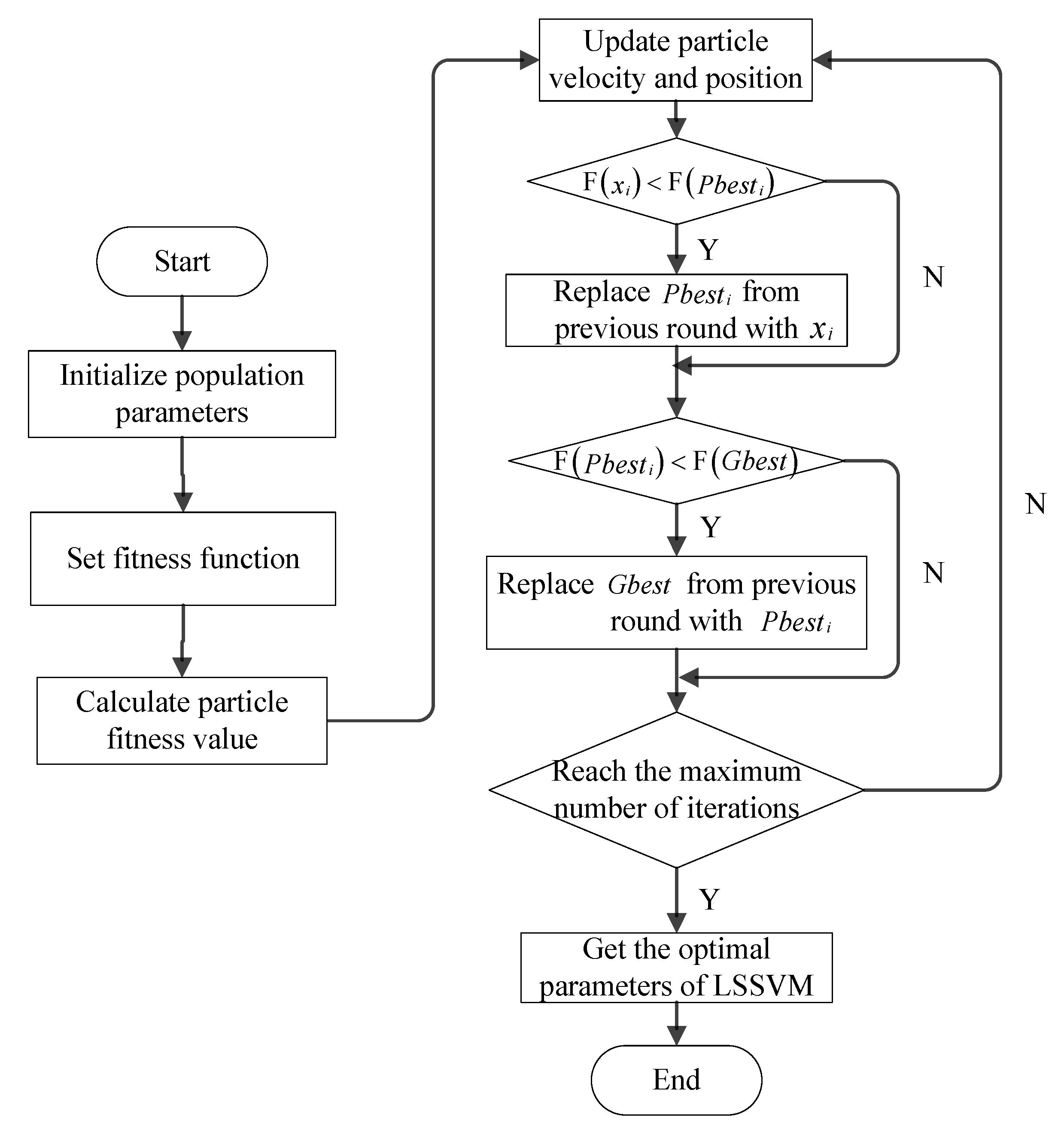
Subject to the radial basis kernel function being selected, the parameters to be optimized for the LSSVM are the penalty coefficient $\gamma$ and the kernel function parameter $\sigma$. A flow chart of the PSO-LSSVM model is shown in Figure 3. The specific optimization steps for the PSO-LSSVM are as follows.

(1)

Set initial parameters, including acceleration factors ${{\displaystyle c}}_1$ and ${{\displaystyle c}}_2$, inertia weights $w$, population size $m$, and maximum number of evolutionary iterations ${{\displaystyle T}}_{\max }$.

(2)

Initialize the population, including the position and velocity vectors of each particle within the initial population.

(3)

Calculate the fitness value $F(x_i)$ for each particle according to the set fitness function $F$, where $i=1,2,\cdots ,m$. If the particle fitness value is better than its own current extreme value ($F(x_i)<F(Pbes{t}_i)$), replace the $Pbes{t}_i$ of the previous round with $x_i$.

(4)

The best fitness value $F(Pbes{t}_i)$ of each particle is compared with the best fitness value $F(Gbest)$ of all particles and, if $F(Pbes{t}_i)<F(Gbest)$, the population’s optimal position $Gbest$ is replaced by $x_i$.

(5)

Update particle state following the position update formula and velocity update formula to update the velocity and position of the particle.

(6)

Check the termination condition of the optimization (i.e., the set maximum number of iterations $T_{\max }$ or the fitness value $F(x_i)<\epsilon$), if it is satisfied, map the globally optimal particle to the penalty coefficient $\gamma$ and the kernel parameter $\sigma$; otherwise, go to step (4) to continue to complete the iterations.

(7)

The optimal parameters are obtained and the final PSO-LSSVM model is established.

Figure 3. Flow chart of the PSO-LSSVM model.

Figure 3. Flow chart of the PSO-LSSVM model.

2.5. The Proposed Qualitative and Quantitative Analysis Strategy

This paper presents a qualitative and quantitative analysis strategy for continuous turbulent gas mixture monitoring. The strategy consists of two main parts, namely a WOA-LSTM method for qualitative identification of the gas mixtures and a PSO-LSSVM method for quantitative estimation of the gas mixtures. A flow chart of the proposed qualitative and quantitative analysis strategy is shown in Figure 4.

As shown in Figure 4a, in order to construct the gas qualitative identification model and gas quantitative prediction model in the proposed strategy, it is necessary to complete the construction of the sample feature set in advance. In the data preprocessing part, the fractional difference method is used to realize the baseline manipulation of the gas sensor array signal, and the data are then normalized. PCA is used to extract features from the preprocessed sensor array signals. The sensor array signal features obtained through the above steps constitute a sample feature set. The sample feature set is divided into a training set and test set proportionally. The qualitative and quantitative analysis strategy for gas mixtures is illustrated in Figure 4b. The modeling process of the gas identification model and gas concentration estimation model is described. In the above model, the optimization of model parameters is considered. In addition, sample selection is vital for building gas identification models and gas concentration prediction models.

3. Results

3.1. Dataset

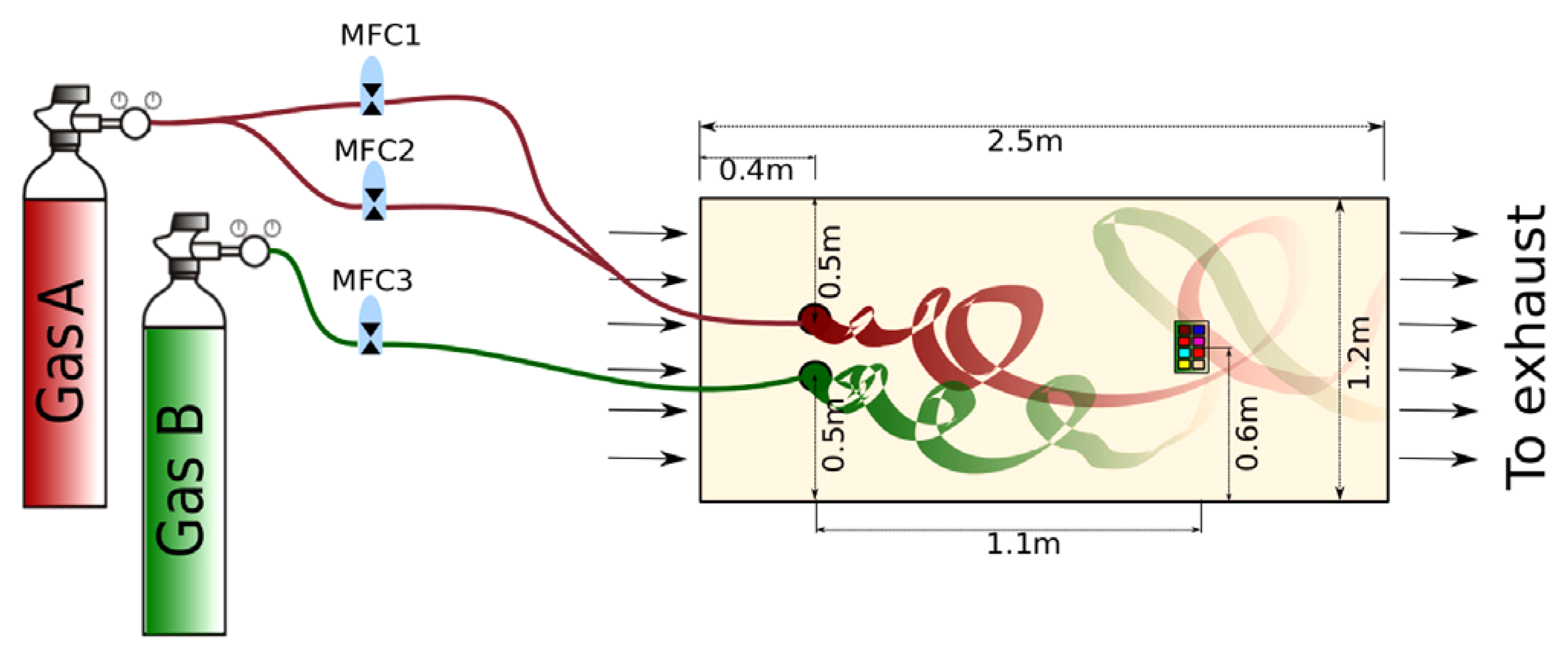
To verify the effectiveness of the qualitative and quantitative analysis strategy proposed in this paper for continuous turbulent gas mixture monitoring, a public dataset provided by the Institute of Biological Circuits at the University of California, San Diego was used as an experimental sample set [18,26]. The public dataset was collected through an open sampling system, which consisted of a wind tunnel with two independent gas sources and a sensor array detection platform with eight built-in MOS gas sensors. The schematic structure of the experimental setup is shown in Figure 5. The types and target gases of the eight MOS gas sensors (provided by Figaro Inc., Osaka, Japan) in the sensor array are shown in

Table 1. Details of the eight MOS gas sensors assembled on the gas sensor array.

Sensor Types	Number of Units	Target Gases
TGS2611	1	CH4
TGS2612	1	CH4, C3H8, C4H10
TGS2610	1	C3H8
TGS2600	1	H2, CO
TGS2602	2	NH3, H2S, VOCs
TGS2620	2	CO, flammable gas, VOCs

. The operating temperature of the sensors is controlled by the voltage applied to the built-in sensors’ heaters. The voltage on the heaters was kept constant at 5 V. The size of the wind tunnel was 2.5 m × 1.2 m × 0.4 m. Two gas sources were included in the wind tunnel. The gas concentration of each plume was controlled by a set of mass flow controllers (mfc). Each source was controlled independently to release selected volatiles at different flow rates, thus producing different concentration levels at the sensor locations. The wind turbine generators created a turbulent flow that continuously moved the introduced volatiles towards the exhaust outlet. The sample was acquired by the response of the gas sensor array. All experimental data in this paper are taken from the above public dataset.

The volatiles under consideration were provided as a mixture of medically dry air with certified concentrations of 2500 ppm ethylene, 1000 ppm methane, and 4000 ppm carbon monoxide. The mixture was produced by releasing ethylene at one source, while the interference plume was produced by releasing methane or carbon monoxide at the source of the interference. Although the gas concentration at the gas source is constant for a given volatile gas, it is important to note that different gas flow rates at the source can lead to plumes of different gas concentrations. In order to estimate the actual concentration at which the detection unit was exposed, the researchers used a GC-MS system as a gold standard. In particular, they utilized a Trace GC ultra coupled with an ISQ single quadrupole MS (Themo Scientific) with a 30 m length, 0.32 mm diameter GS-GASPRO chromatogram column (Agilent) [26].

Table 2. Average estimated concentrations of the three gases at different flow rates obtained by gas chromatography-mass spectrometry.

Volatile Gases	Flow Rate (sccm)	Estimated Concentration (ppm)
Ethylene@2500 ppm	20	96
	14	46
	8	31
Carbon monoxide @4000 ppm	200	460
	180	397
	140	270
Methane@1000 ppm	300	131
	200	115
	100	51

shows the average concentrations of the three gases in the wind tunnel at different flow rates estimated by gas chromatography-mass spectrometry (GC-MS) under fan operation. The total duration of each measurement was 300 s. During the first 60 s, no gas was released at the source. At t = 60 s, both sources started releasing the corresponding volatile fraction at the specified flow rate. The gas release duration was 180 s. Finally, the system reverted to the baseline of 60 s. Throughout the experiment, the sensor signals were continuously acquired every 20 ms, generating eight time series which indicated the gas conditions presented to the sensor. The public dataset collected by the gas acquisition system contains a total of 180 text files, of which 72 data sample files correspond to three single gases. The remaining 108 data sample files correspond to mixed gases, which are ethylene-carbon monoxide and ethylene-methane mixed gases.

Each sample is the response signal of the gas sensor array to two gas mixtures with different concentration levels (n: 0, L: Low, M: Medium, H: High). During the experiments, the average concentration levels of the individual gas components in the turbulent gas mixtures were estimated by means of a gas chromatography-mass spectrometry (GC-MS) system. Detailed information regarding the mixed gas samples in the dataset is shown in

Table 3. Sample distribution in the dataset along with rate of chemical release (in sccm) and corresponding induced gas concentration level (in ppm) in the vicinity of the sensors. In total, 180 measurements were performed. The labels H, M, L, and n indicate high, medium, low, and zero concentrations of the corresponding volatiles, respectively.

Volatiles			Ethylene@2500 ppm
			20 sccm	14 sccm	8 sccm	0 sccm
			H:96 ppm	M:46 ppm	L:31 ppm	n:0 ppm
Carbon Monoxide @4000 ppm	200 sccm	H: 460 ppm	6	6	6	6
	140 sccm	M: 397 ppm	6	6	6	6
	800 sccm	L: 270 ppm	6	6	6	6
	0 sccm	n: 0 ppm	6	6	6	—
Methane @1000 ppm	300 sccm	H: 131 ppm	6	6	6	6
	200 sccm	M: 115 ppm	6	6	6	6
	100 sccm	L: 51 ppm	6	6	6	6
	0 sccm	n: 0 ppm	6	6	6	—

. As shown in Table 3, the experiment was divided into 30 batches, and six independent repeated experiments were carried out for each set with fixed concentrations of two mixed gases. Response curves of ethylene and carbon monoxide gas mixtures are shown in Figure 6. In Figure 6, it can be seen that the response signal of the sensor array in the case of continuous turbulent gas has randomness and dynamic characteristics that create a challenge for the subsequent identification and concentration estimation of the gas mixture components.

3.2. Training Sample Selection Strategy

The strategy proposed in this paper for the qualitative and quantitative analysis of gas mixtures is implemented using pattern recognition methods. Appropriate training sample selection can have a positive impact on the performance of a gas detection model. Particularly in turbulent gas mixtures, the dynamics of the gas flow make the detection of the composition of the gas mixtures even more complex. This part uses different training sample selection strategies to implement the modelling and aims to analyze the impact of different sample selections on the qualitative and quantitative analysis of turbulent gas mixtures.

3.2.1. Sample Selection Strategy for Qualitative Analysis

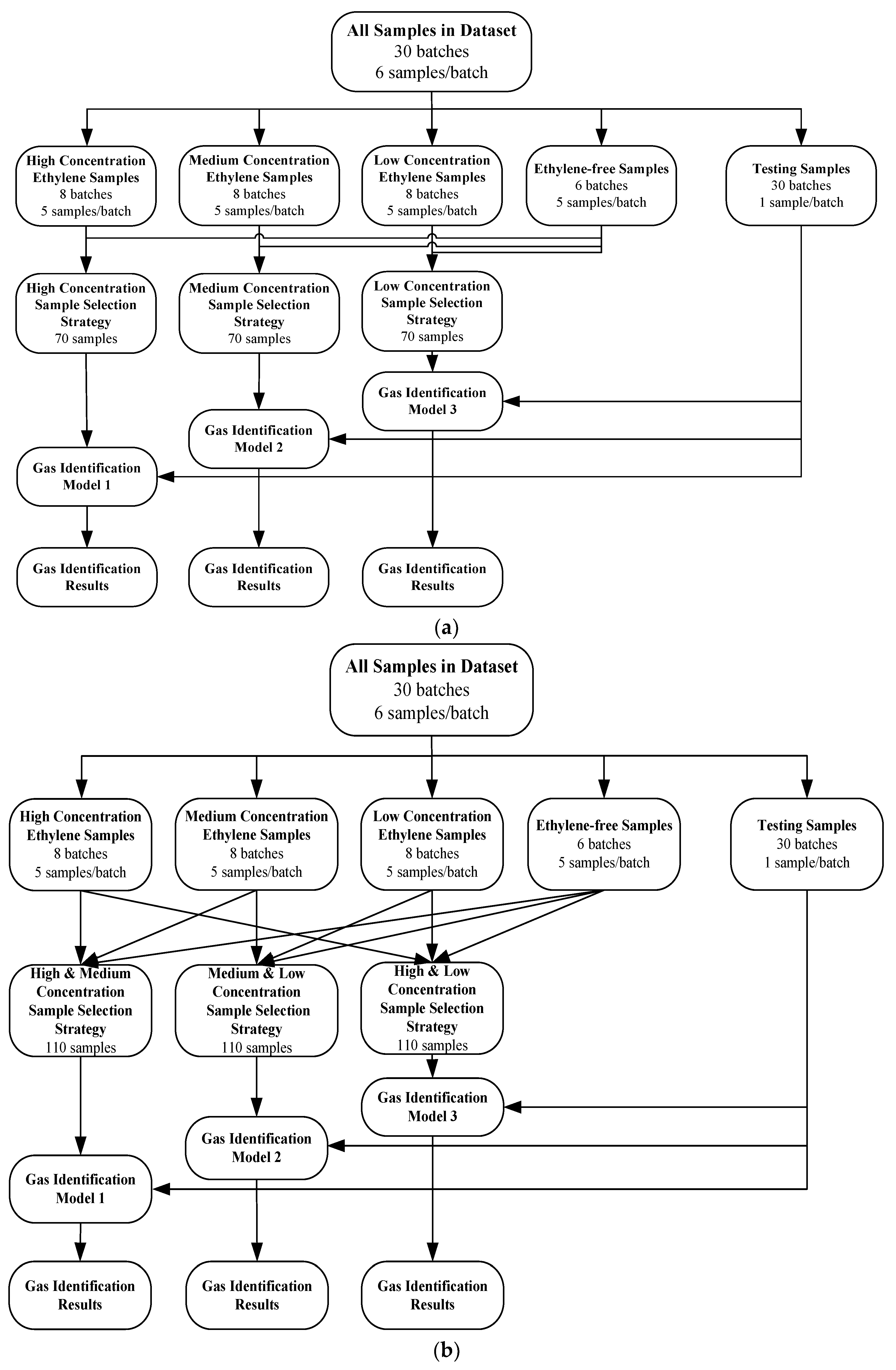
In real world atmospheric environments, gases are present as a mixture, and the gas detection model needs to identify gas composition in the presence of gas turbulence. Therefore, two gas identification scenarios are respectively considered, namely identifying a certain gas component in the gas mixtures and identifying the composition of components in the gas mixtures. Figure 7 shows the two different training sample selection strategies employed in this paper to identify a certain gas component contained in the gas mixtures. In order to identify the presence of ethylene in the gas mixtures, the training samples should consist of gas samples with ethylene and without ethylene. As shown in Figure 7a, the single-concentration level sample selection strategy selects the high-concentration, medium-concentration, and low-concentration ethylene mixed gas samples and ethylene-free samples as the training samples (70 samples) to establish the gas identification model. The testing samples (30 samples) are used to verify the ethylene gas identification performance of the qualitative analysis model. In Figure 7b, the compound-concentration level sample selection strategy further expands the training samples and selects samples of any two concentration levels in high-concentration, medium-concentration, and low-concentration ethylene gases to combine with ethylene-free samples in order to train the gas identification model. Compared to the sample selection strategy in Figure 7a, the number of training samples is increased from 70 to 110. In addition, the size of the testing set is still 30 samples to validate the performance of the gas identification model.

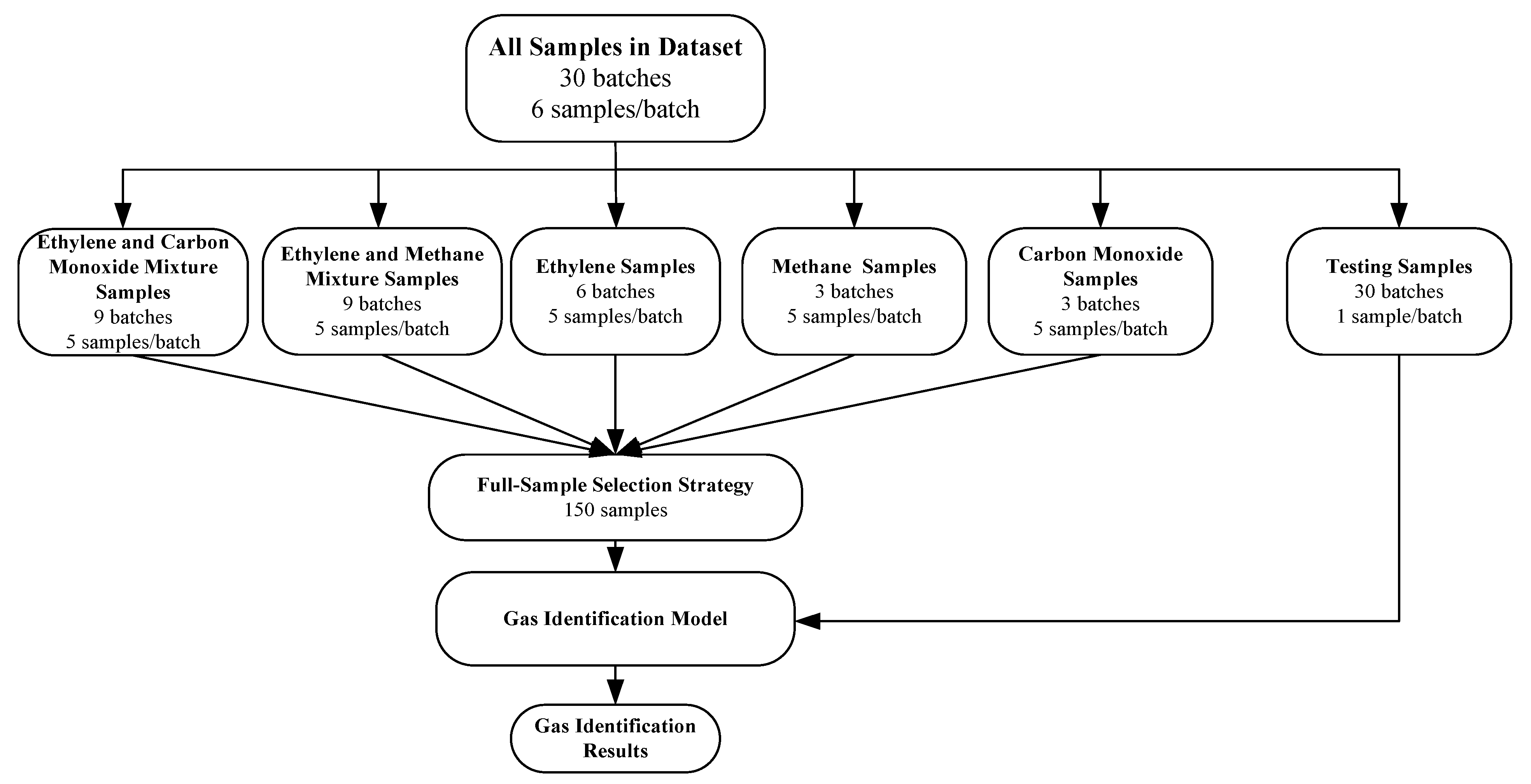
In order to further accurately identify the composition of components in turbulent gas mixtures, this paper adopts the full-sample selection strategy shown in Figure 8 and analyzes its effect on gas mixture identification. The strategy divides the samples in the original dataset into five types, namely the mixture of ethylene and carbon monoxide, the mixture of ethylene and methane, pure ethylene, pure methane, and pure carbon monoxide. The above gas samples are divided into training samples and testing samples according to a fixed proportion in order to model and verify the gas mixture identification model. This strategy makes full use of all the samples in the dataset, containing mixtures of ethylene gases at different concentration levels.

3.2.2. Sample Selection Strategy for Quantitative Analysis

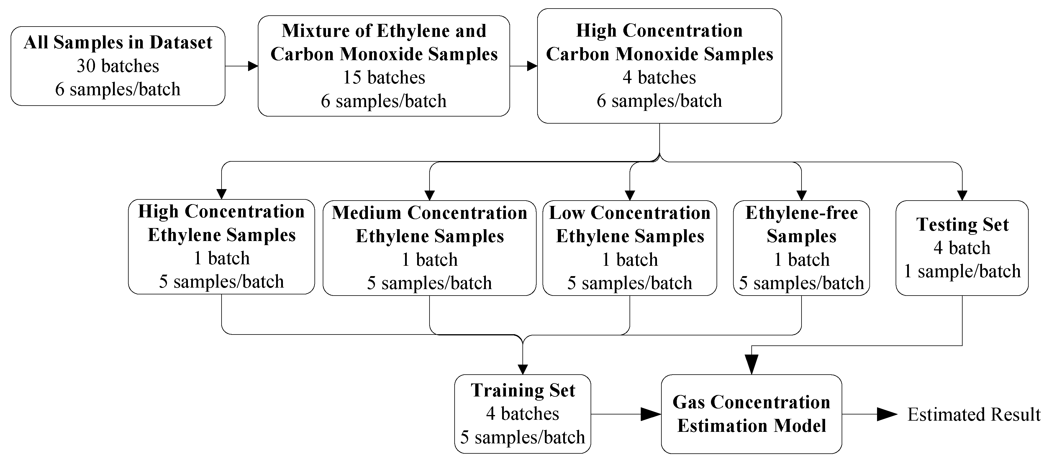
Estimating the concentration of gas components in turbulent gas mixtures is an important function of gas detection models. Due to the complex composition of mixed gas and the cross-sensitivity of gas sensors, multiple regression methods are generally used for modeling. Therefore, sample selection has a significant impact on the performance of gas detection models. Estimating the target gas concentration under the background gas is one of the important functions of the gas detection model. The sample selection strategy, using ethylene as the target gas under the condition of high-concentration carbon monoxide as the background gas, is shown in Figure 9. The gas concentration prediction model was modeled by selecting the mixed gas samples of ethylene and high concentrations of carbon monoxide from all samples in the dataset. The gas concentration prediction model is modelled on a mixture of ethylene and high concentrations of carbon monoxide selected from all samples in the dataset. The sample selection strategy for estimating the concentration of a target gas in other gas mixtures is consistent with the selection strategy depicted in Figure 9.

The sample selection strategy described in Figure 9 can only be applied when the background gas concentration is fixed, which limits the range of applications for the mixture concentration estimation models trained with it. Therefore, a full-sample selection strategy for mixed gas concentrations is proposed in this paper. The full-sample selection strategy for estimating ethylene concentration is shown in Figure 10. This sample selection strategy covers all samples in the dataset. The sample selection strategy ignores information on the type and concentration of the background gas and only takes into account the presence and absence of the target gas to form the training set. The sample selection strategy significantly increases the size of the training set. The sample selection strategy is consistent with the rationale depicted in Figure 10 regarding the estimation of other gas concentrations in the dataset.

3.3. Experimental Results

3.3.1. Qualitative Gas Mixture Identification Results

In order to demonstrate the effectiveness of the WOA-LSTM-based mixture identification method proposed in this paper, different sample selection strategies were used to verify the effectiveness of mixture identification. The parameters for the WOA-optimized LSTM in the gas recognition model used in this paper were set as 21 neurons in the hidden layer and a learning rate of 0.0047.

The average ethylene gas identification accuracy of the single-concentration sample selection strategy depicted in Figure 7a is shown in

Table 4. Average ethylene gas identification accuracy of WOA-LSTM with the single-concentration level sample selection strategy. The training samples were selected from high-concentration, medium-concentration, or low-concentration ethylene samples.

Sample Selection Strategies	Average Identification Accuracy (%)
High-concentration sample selection strategy	88.17 ± 6.09
Medium-concentration sample selection strategy	91.56 ± 3.30
Low-concentration sample selection strategy	94.40 ± 2.57

. While the average ethylene gas identification accuracy with compound ethylene concentration sample selection strategies as described in Figure 7b is shown in

Table 5. Average ethylene gas identification accuracy of WOA-LSTM with compound ethylene concentration sample selection strategies. The training samples were selected from high- and low-concentration, medium- and low-concentration, or high- and medium-concentration ethylene samples.

Sample Selection Strategies	Average Identification Accuracy (%)
High- and low-concentration sample selection strategy	94.00 ± 2.08
Medium- and low-concentration sample selection strategy	96.39 ± 1.48
High- and medium-concentration sample selection strategy	93.39 ± 3.22

. From the above experimental results, it can be seen that both sample selection strategies shown in Figure 7 have a high accuracy rate when identifying ethylene gas.

Table 6. Average identification accuracy of different gas recognition models with compound ethylene concentration sample selection strategies.

Models	SVM	KNN	BP	Softmax	LSTM	WOA-LSTM
Average identification accuracy (%)	88.93 ± 2.25	95.91 ± 1.65	86.21 ± 3.17	86.70 ± 2.78	94.67 ± 1.98	96.39 ± 1.48

compares the average identification accuracy of different gas identification models with medium- and low-concentration sample selection strategies, and the results show that the WOA-LSTM-based gas identification model proposed in this paper has the highest gas identification result. The average recognition accuracy of WOA-LSTM is 96.39%, while the average recognition accuracy of LSTM is 94.67%.

In order to further identify the composition of turbulent gas mixtures, a more comprehensive sample is required to establish the gas identification model. This paper adopts the full-sample selection strategy shown in Figure 8 to illustrate the multi-gas component identification performance of the WOA-LSTM model. The gas identification models were tested using a mixture of ethylene and methane, a mixture of ethylene and carbon monoxide, ethylene, methane, and carbon monoxide. The identification accuracy of WOA-LSTM for five gas components is shown in

Table 7. Identification accuracy of WOA-LSTM for different gas components.

Gas Categories	Ethylene and Methane	Ethylene and Carbon Monoxide	Ethylene	Methane	Carbon Monoxide
Identification accuracy (%)	95.24 ± 2.91	94.97 ± 3.21	90.48 ± 2.28	95.24 ± 2.51	95.24 ± 3.03

. From the experimental results, it can be seen that the proposed WOA-LSTM method is able to identify the components of turbulent gas mixtures with an identification accuracy of over 90%.

In order to demonstrate the superiority of the proposed WOA-LSTM method for qualitative identification of turbulent mixed gases, SVM, KNN, BP, Softmax, and LSTM were introduced as comparison methods in this paper, and the mixed gas multi-classification results of WOA-LSTM were compared with those of the other five methods, as shown in

Table 8. Average identification accuracy of different gas identification models for multi-gas components with the full-sample selection strategy.

Models	SVM	KNN	BP	Softmax	LSTM	WOA-LSTM
Identification accuracy (%)	72.2 ± 2.08	76.84 ± 3.05	84.45 ± 3.43	66.7 ± 3.73	88.32 ± 2.39	94.61 ± 2.74

. It can be seen that the WOA-LSTM method has the highest recognition accuracy compared to other gas identification models.

3.3.2. Quantitative Gas Mixture Estimation Results

To illustrate the performance of the PSO-LSSVM model regarding turbulent gas mixture concentration prediction, the experiments were conducted using different sample selection strategies.

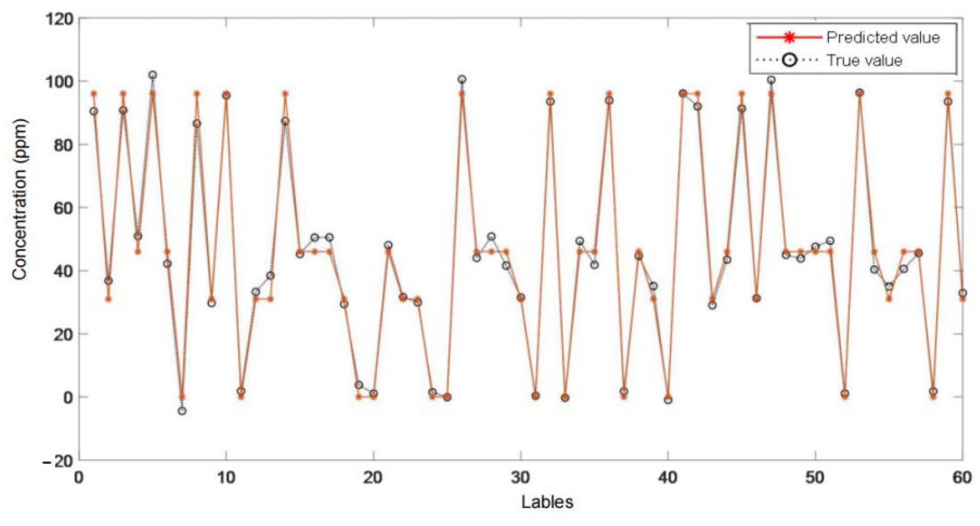
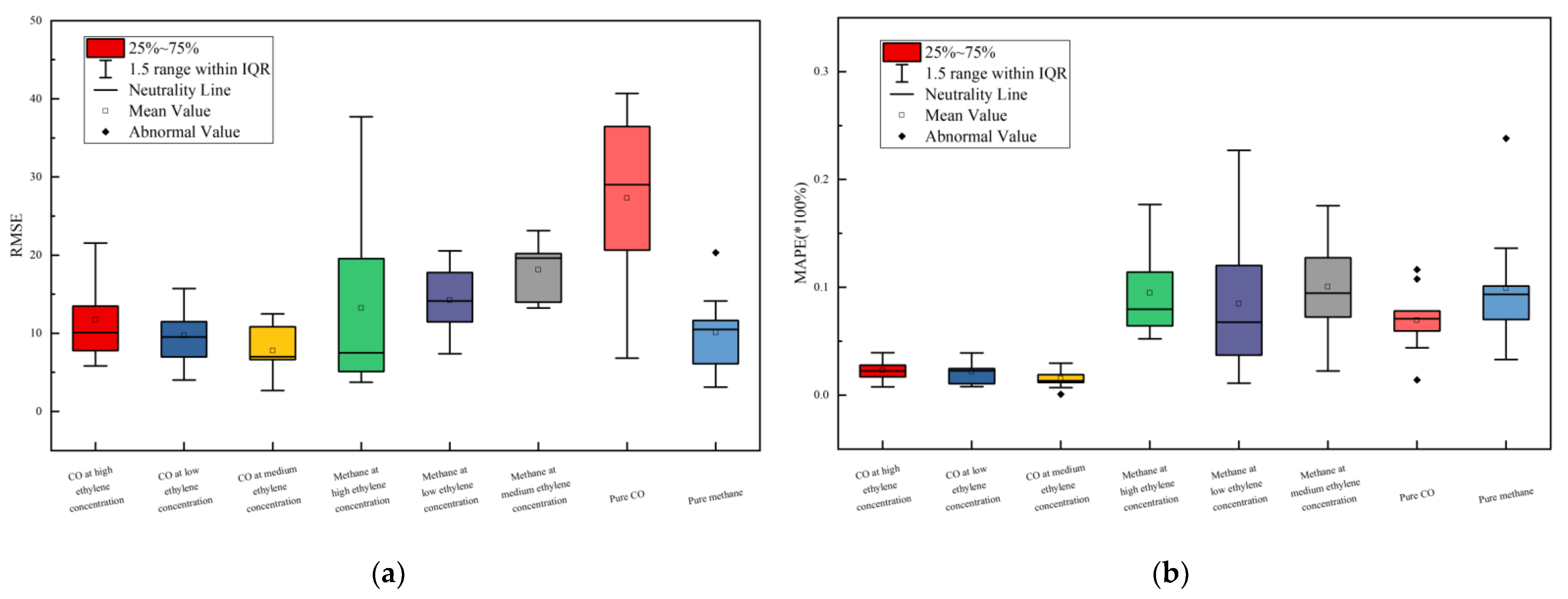
First, this paper provides experimental validation of the effectiveness of PSO-LSSVM in predicting the target gas concentration for a given background gas in the mixture. Figure 11 shows the predicted results of ethylene gas concentration using the PSO-LSSVM method under the condition of a high concentration of carbon monoxide as the background gas and the sample selection strategy shown in Figure 9. The box plots of ethylene concentration prediction errors (RMSE and MAPE) under the condition of a high concentration of carbon monoxide as the background gas are shown in Figure 12. The concentration prediction results of ethylene with carbon monoxide and methane as the background gas are shown in

Table 9. Concentration prediction results for carbon monoxide and methane with ethylene as the background gas.

Target Gas	RMSE	MAPE (%)
Ethylene under the background of a high concentration of carbon monoxide	4.7212	5.49
Ethylene under the background of a medium concentration of carbon monoxide	4.1134	5.38
Ethylene under the background of a low concentration of carbon monoxide	3.0786	5.10
Ethylene under the background of a high concentration of methane	2.8608	4.56
Ethylene under the background of a medium concentration of methane	2.8826	4.03
Ethylene under the background of a low concentration of methane	3.7376	4.82
Pure ethylene	4.3210	7.58

.

In addition, the experiment uses ethylene as the background gas and uses PSO-LSSVM to predict carbon monoxide and methane gas concentrations. The box plots of carbon monoxide and methane prediction errors (RMSE and MAPE) under the condition of ethylene as the background gas are shown in Figure 13. The concentration prediction results for carbon monoxide and methane with ethylene as the background gas are shown in Table 9.

Combining the experimental results in Table 9 and

Table 10. Concentration prediction results for carbon monoxide and methane with ethylene as the background gas.

Target Gas	RMSE	MAPE (%)
Carbon monoxide with high-concentration ethylene as the background gas	8.3818	2.38
Carbon monoxide with medium-concentration ethylene as the background gas	8.2541	2.26
Carbon monoxide with low-concentration ethylene as the background gas	8.2358	2.19
Pure carbon monoxide	27.3094	6.94
Methane with high-concentration ethylene as the background gas	16.9220	9.47
Methane with medium-concentration ethylene as the background gas	18.4146	10.06
Methane with low-concentration ethylene as the background gas	14.7585	8.49
Pure methane	10.0737	9.88

,

Table 11. Overall prediction effect of the PSO-LSSVM model on turbulent gas mixtures.

Target Gas	RMSE	MAPE (%)
Ethylene	3.6736	5.28
Methane	15.0442	9.48
Carbon monoxide	13.0453	3.44

shows the overall prediction effect of the PSO-LSSVM model on turbulent gas mixtures. In order to further illustrate the composition prediction performance of the PSO-LSSVM model for turbulent mixed gas, this paper uses the SVM and LSSVM methods to predict the ethylene concentration in the mixed gas under the same conditions. The comparative experimental results are shown in

Table 12. Concentration prediction results of ethylene gas in mixed gas using different concentration prediction methods.

Target Gas	RMSE	MAPE (%)
PSO-LSSVM	3.6736	5.28
SVM	15.0442	9.16
LSSVM	9.941	7.61

.

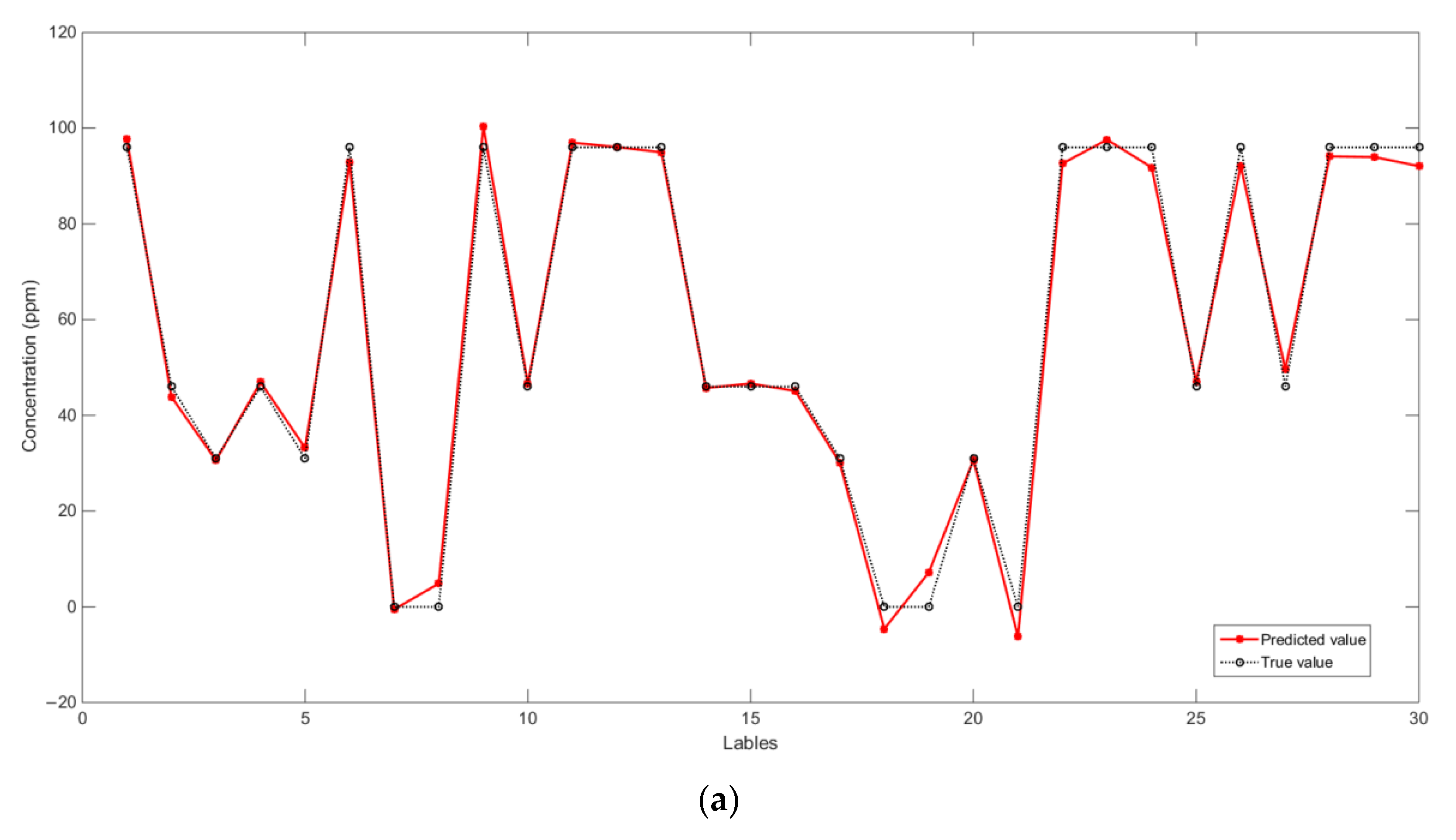
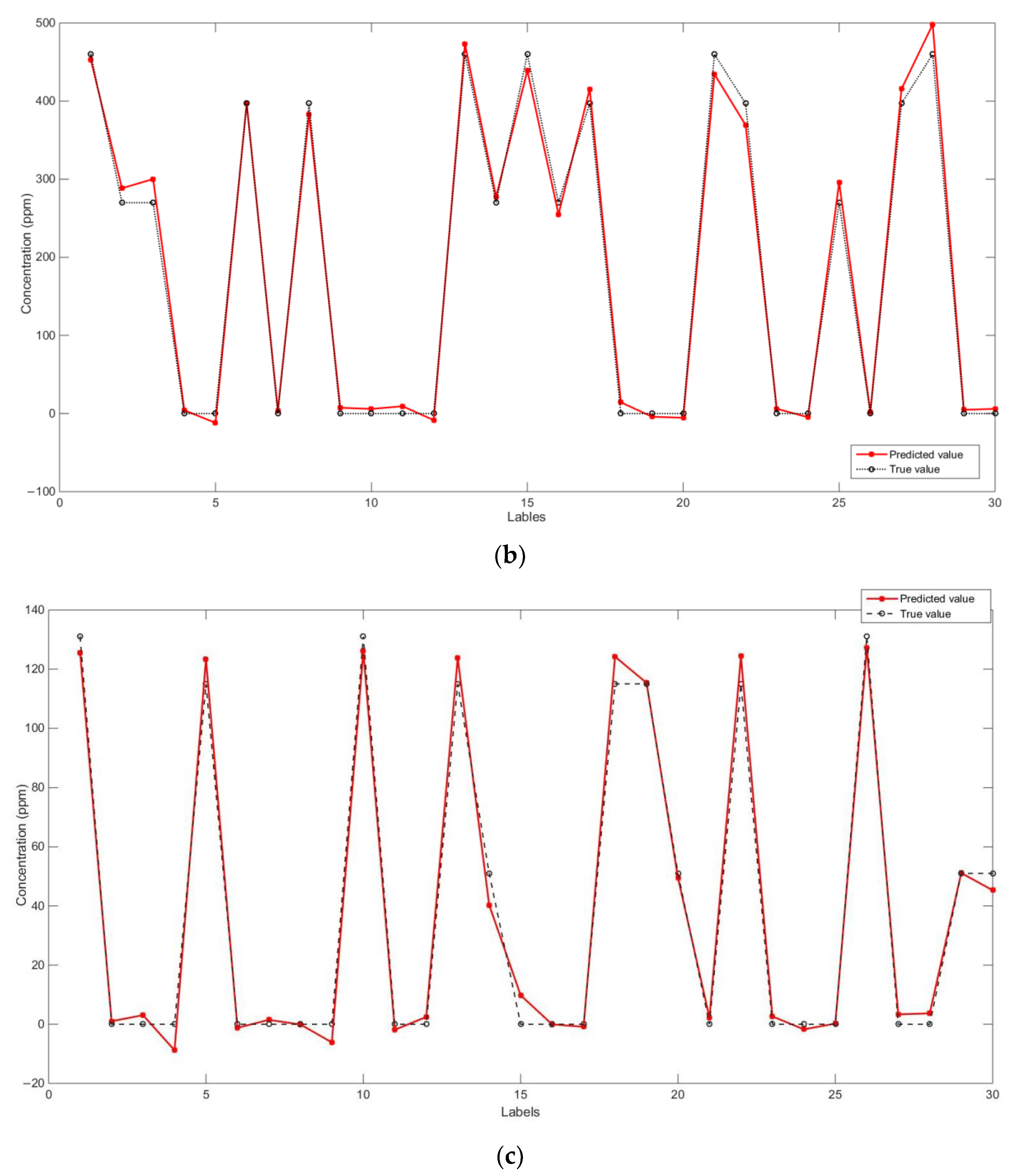
Second, the prediction results for the turbulent mixed gas concentration obtained by the PSO-LSSVM model under the condition of the full-sample selection strategy being used are verified by experiments. The prediction results for three gas concentrations under the full-sample selection strategy are shown in Figure 14. A comparison of results of the true and predicted concentrations of ethylene, methane, and carbon monoxide in the test samples is shown in the graphs. Evidently, the concentration prediction model based on PSO-LSSVM has good prediction accuracy.

Table 13. Prediction results for three gas concentrations with the full-sample selection strategy.

Target Gas	RMSE	MAPE (%)
Ethylene	3.2609	4.19
Methane	3.3391	1.29
Carbon monoxide	5.1919	2.58

evaluates the prediction accuracy for each of the three gases using RMSE and MAPE. In order to further illustrate the performance of the PSO-LSSVM-based gas concentration prediction model,

Table 14. Ethylene concentration prediction results of different algorithms under the full-sample selection strategy.

Target Gas	RMSE	MAPE (%)
SVM	12.8261	7.21
LSSVM	8.2998	6.73
PSO-LSSVM	3.2609	4.19

compares the prediction results of different algorithms for ethylene gas concentrations. The results show that PSO-LSSVM has higher prediction accuracy for ethylene gas concentrations compared to the SVM and LSSVM methods.

4. Discussion

By describing the experimental results of the qualitative gas mixture identification model in Section 3.3.1, it can be seen that the proposed WOA-LSTM-based turbulent gas mixture identification model has good gas identification accuracy. In Table 4, Using a single-concentration level sample selection strategy for ethylene gas identification shows that the highest average identification accuracy is obtained by training the WOA-LSTM model with low-concentration ethylene samples. As can be seen in Table 3, the medium- and low-concentration samples are closer in ethylene concentration levels; therefore, the WOA-LSTM method is more likely to lead to confusion when modeling the medium- and low-concentration samples during gas identification. Modelling the WOA-LSTM method with high concentrations of ethylene samples does not achieve the desired identification results in the identification of low and medium concentrations of ethylene samples. This is mainly because the response of the gas sensor array is more significant for high-concentration ethylene samples, and the WOA-LSTM model trained using this response signal is less sensitive to low- and medium-concentration ethylene samples. In order to improve the gas identification performance of the WOA-LSTM model, a compound sample selection strategy is used for modeling WOA-LSTM, and the experimental results are shown in Table 5. The classification accuracy of the sample selection strategy with low-concentration vinyl samples improved, and the sample selection strategy with a combination of medium- and low-concentration samples had the best classification accuracy. The sample selection strategy with a combination of medium and low concentrations was chosen, and the corresponding samples were input into the LSTM model, SVM, KNN, BP neural network, and Softmax classification model. The classification results corresponding to these five algorithm models were compared and analyzed with regard to WOA-LSTM, and the results are shown in Table 6. Among the six classification algorithms, the LSTM and WOA-LSTM models have a significant advantage in terms of classification accuracy, as the LSTM model is better able to handle long time series data and is more conducive to the identification of mixed gas components. The WOA-LSTM identification model achieves the highest recognition rate, with a 1.72% increase in accuracy compared to the LSTM model, demonstrating the positive effect of the WOA optimization algorithm on the LSTM. In order to explore the ability of WOA-LSTM to identify more components in a mixture, a full-sample selection strategy was used for modelling and the experimental results are shown in Table 7. It can be seen that the WOA-LSTM model can distinguish the five gas components quite accurately. The average of the classification results was obtained after several training sessions, and the final multi-classification accuracy of WOA-LSTM for the mixed gases was 94.61%. In addition, Table 8 illustrates that the WOA-LSTM model trained using the full-sample training strategy had the highest recognition accuracy for the different gas components compared to the other methods.

The PSO-LSSVM model has good turbulent gas mixture concentration prediction, as can be seen from the experimental results of mixed gas component concentration prediction in Section 3.3.2. Two practical scenarios for use are discussed, namely the prediction of the concentration of a particular gas with a fixed background gas and the prediction of the concentration of each component in a gas mixture. Analysis of Figure 11 and Figure 12, and Table 9 shows that the RMSEs and MAPEs of the predicted ethylene gas concentrations are low under the conditions where carbon monoxide and methane gases are used as background gases. Furthermore, Figure 13 and Table 10 show that the predictions of other gas concentrations also have good accuracy with ethylene as the background gas. It is possible through analysis of the experimental results to identify that the PSO-LSSVM model has a large deviation in prediction for pure gases, mainly due to the large range of pure gas concentrations. As a result, the overall concentration predictions depicted in Table 11 show a slight increase compared to Table 9 and Table 10. Table 12 compares the results of SVM, LSSVM, and PSO-LSSVM for the prediction of mixed gas concentrations and shows that the PSO-LSSVM model has the smallest RMSE and MAPE, indicating that the performance of the LSSVM model has been enhanced by PSO. In view of this, to further improve the prediction accuracy, the PSO-LSSVM model was trained using a full-sample selection strategy in this paper. The full-sample selection strategy expands the number of training samples and can obtain a more performant gas concentration prediction model. As shown in Table 13 and Table 14, it can be seen that training the PSO-LSSVM model using a full-sample selection strategy can further improve the accuracy of turbulent gas mixture concentration estimation.

5. Conclusions

Electronic nose systems with chemical sensors as core components have potential applications in a wide range of fields; however, there are still a number of problems that need to be solved. This paper investigates a qualitative and quantitative analysis strategy for continuous turbulent mixed gas monitoring in an attempt to address the key bottleneck in the use of electronic nose systems in natural atmospheric environments. The proposed strategy combines WOA-LSTM and PSO-LSSVM to achieve qualitative identification and quantitative prediction of mixed gas components, respectively. The effectiveness of the proposed strategy was validated using a public dataset provided by the Institute of Biological Circuits at the University of California, San Diego. Moreover, this paper discusses the experimental results of qualitative identification and quantitative prediction of gas mixtures under different sample selection strategies. With different sample selection strategies, the proposed strategies are all able to achieve a certain degree of accuracy in gas identification and concentration estimation. It can be seen that the full-sample selection strategy achieves the best detection results due to the inclusion of more experimental samples. The proposed qualitative and quantitative analysis strategy for continuous turbulent gas mixture monitoring has high detection accuracy and is capable of initial application in subsequent atmospheric environmental pollution monitoring, public safety monitoring, and other fields. However, the research in this paper also has the limitation that no experimental verification has been carried out for frequent changes in the concentration of the gas source, which will be a direction for future research.

References

1. Jing, Y.Q.; Meng, Q.H.; Qi, P.F.; Cao, M.L.; Zeng, M.; Ma, S.G. A bioinspired neural network for data processing in an electronic nose. IEEE Trans. Instrum. Meas. 2016, 65, 2369–2380. [Google Scholar] [CrossRef]
2. Karakaya, D.; Ulucan, O.; Turkan, M. Electronic nose and its applications: A survey. Int. J. Autom. Comput. 2020, 17, 179–209. [Google Scholar] [CrossRef] [Green Version]
3. Sankaran, S.; Khot, L.R.; Panigrahi, S. Biology and applications of olfactory sensing system: A review. Sens. Actuators B: Chem. 2012, 171, 1–17. [Google Scholar] [CrossRef]
4. Loutfi, A.; Coradeschi, S.; Mani, G.K.; Shankar, P.; Rayappan, J.B.B. Electronic noses for food quality: A review. J. Food Eng. 2015, 144, 103–111. [Google Scholar] [CrossRef]
5. Kumar, A.; Kim, H.; Hancke, G.P. Environmental monitoring systems: A review. IEEE Sens. J. 2012, 13, 1329–1339. [Google Scholar] [CrossRef] [Green Version]
6. Covington, J.A.; Marco, S.; Persaud, K.C.; Schiffman, S.S.; Nagle, H.T. Artificial Olfaction in the 21 st Century. IEEE Sens. J. 2021, 21, 12969–12990. [Google Scholar] [CrossRef]
7. Hackner, A.; Oberpriller, H.; Ohnesorge, A.; Hechtenberg, V.; Müller, G. Heterogeneous sensor arrays: Merging cameras and gas sensors into innovative fire detection systems. Sens. Actuators B Chem. 2016, 231, 497–505. [Google Scholar] [CrossRef]
8. Hassan, M.; Umar, M.; Bermak, A. Computationally efficient weighted binary decision codes for gas identification with array of gas sensors. IEEE Sens. J. 2016, 17, 487–497. [Google Scholar] [CrossRef]
9. Gutierrez-Osuna, R. Pattern analysis for machine olfaction: A review. IEEE Sens. J. 2002, 2, 189–202. [Google Scholar] [CrossRef] [Green Version]
10. Marco, S.; Gutierrez-Galvez, A. Signal and data processing for machine olfaction and chemical sensing: A review. IEEE Sens. J. 2012, 12, 3189–3214. [Google Scholar] [CrossRef]
11. Fan, S.; Li, Z.; Xia, K.; Hao, D. Quantitative and qualitative analysis of multicomponent gas using sensor array. Sensors 2019, 19, 3917. [Google Scholar] [CrossRef] [PubMed] [Green Version]
12. Laref, R.; Losson, E.; Sava, A.; Siadat, M. On the optimization of the support vector machine regression hyperparameters setting for gas sensors array applications. Chemom. Intell. Lab. Syst. 2019, 184, 22–27. [Google Scholar] [CrossRef]
13. Gamboa, J.C.R.; da Silva, A.J.; Araujo, I.C. Validation of the rapid detection approach for enhancing the electronic nose systems performance, using different deep learning models and support vector machines. Sens. Actuators B Chem. 2021, 327, 128921. [Google Scholar] [CrossRef]
14. Chen, Z.; Zheng, Y.; Chen, K.; Li, H.; Jian, J. Concentration estimator of mixed VOC gases using sensor array with neural networks and decision tree learning. IEEE Sens. J. 2017, 17, 1884–1892. [Google Scholar] [CrossRef]
15. Bakiler, H.; Güney, S. Estimation of Concentration Values of Different Gases Based on Long Short-Term Memory by Using Electronic Nose. Biomed. Signal Process. Control 2021, 69, 102908. [Google Scholar] [CrossRef]
16. Chu, J.; Li, W.; Yang, X.; Wu, Y.; Wang, D.; Yang, A.; Yuan, H.; Wang, X.; Li, Y.; Rong, M. Identification of gas mixtures via sensor array combining with neural networks. Sens. Actuators B Chem. 2021, 329, 129090. [Google Scholar] [CrossRef]
17. Monroy, J.G.; Palomo, E.J.; López-Rubio, E.; Gonzalez-Jimenez, J. Continuous chemical classification in uncontrolled environments with sliding windows. Chemom. Intell. Lab. Syst. 2016, 158, 117–129. [Google Scholar] [CrossRef]
18. Fonollosa, J.; Rodríguez-Luján, I.; Trincavelli, M.; Vergara, A.; Huerta, R. Chemical discrimination in turbulent gas mixtures with mox sensors validated by gas chromatography-mass spectrometry. Sensors 2014, 14, 19336–19353. [Google Scholar] [CrossRef] [Green Version]
19. Fonollosa, J.; Sheik, S.; Huerta, R.; Marco, S. Reservoir computing compensates slow response of chemosensor arrays exposed to fast varying gas concentrations in continuous monitoring. Sens. Actuators B Chem. 2015, 215, 618–629. [Google Scholar] [CrossRef]
20. Vergara, A.; Fonollosa, J.; Mahiques, J.; Trincavelli, M.; Rulkov, N.; Huerta, R. On the performance of gas sensor arrays in open sampling systems using Inhibitory Support Vector Machines. Sens. Actuators B Chem. 2013, 185, 462–477. [Google Scholar] [CrossRef]
21. Hochreiter, S.; Schmidhuber, J. Long short-term memory. Neural Comput. 1997, 9, 1735–1780. [Google Scholar] [CrossRef]
22. Suykens, J.A.K.; Vandewalle, J. Least squares support vector machine classifiers. Neural Process. Lett. 1999, 9, 293–300. [Google Scholar] [CrossRef]
23. Guo, Z.; Bai, G. Application of least squares support vector machine for regression to reliability analysis. Chin. J. Aeronaut. 2009, 22, 160–166. [Google Scholar] [CrossRef] [Green Version]
24. Mirjalili, S.; Lewis, A. The whale optimization algorithm. Adv. Eng. Softw. 2016, 95, 51–67. [Google Scholar] [CrossRef]
25. Poli, R.; Kennedy, J.; Blackwell, T. Particle swarm optimization. Swarm Intell. 2007, 1, 33–57. [Google Scholar] [CrossRef]
26. Fonollosa, J.; Rodríguez-Luján, I.; Trincavelli, M.; Huerta, R. Data set from chemical sensor array exposed to turbulent gas mixtures. Data Brief 2015, 3, 216–220. [Google Scholar] [CrossRef]
Figure 1. The structure of a standard LSTM network.
Chemosensors 10 00499 g001
Figure 4. Flow chart of the proposed qualitative and quantitative analysis strategy. (a) The data preprocessing and feature extraction performed to create the sample feature set. (b) The modeling process of the WOA-LSTM model and PSO-LSSVM model.
Chemosensors 10 00499 g004
Figure 5. Schematic diagram of the experimental setup of the public dataset used in this paper. The wind tunnel includes two gas sources that generate two independent gas plumes. The facility collected sensor responses when placed in a turbulent environment [14].
Chemosensors 10 00499 g005
Figure 6. Response curves of ethylene and carbon monoxide gas mixtures.
Chemosensors 10 00499 g006
Figure 7. Two different training sample selection strategies for identifying a certain gas component in the gas mixtures. (a) Single-concentration level sample selection strategy; (b) compound-concentration level sample selection strategy.
Chemosensors 10 00499 g007
Figure 8. Full-sample selection strategy for gas mixture identification.
Chemosensors 10 00499 g008
Figure 9. Sample selection strategy for ethylene as a target gas under the conditions of high-concentration carbon monoxide as a background gas.
Chemosensors 10 00499 g009
Figure 10. Full-sample selection strategy for estimating ethylene concentration.
Chemosensors 10 00499 g010
Figure 11. Predicted results of ethylene gas concentration using the PSO-LSSVM method under the condition of a high concentration of carbon monoxide as the background gas.
Chemosensors 10 00499 g011
Figure 12. Box plots of ethylene concentration prediction errors under the condition of a high concentration of carbon monoxide as the background gas. (a) RMSE; (b) MAPE.
Chemosensors 10 00499 g012
Figure 13. Box plots of carbon monoxide and methane concentration prediction errors under the condition of ethylene as the background gas. (a) RMSE; (b) MAPE.
Chemosensors 10 00499 g013
Figure 14. Prediction results for three gas concentrations under the full-sample selection strategy. (a) Comparison of predicted and real ethylene concentration; (b) comparison of predicted and true values of carbon monoxide concentration; (c) comparison of predicted and true methane concentrations.
Chemosensors 10 00499 g014aChemosensors 10 00499 g014b