
Forecasting Hospital Readmissions with Machine Learning


 and
and 
Abstract
:1. Introduction
2. The Data
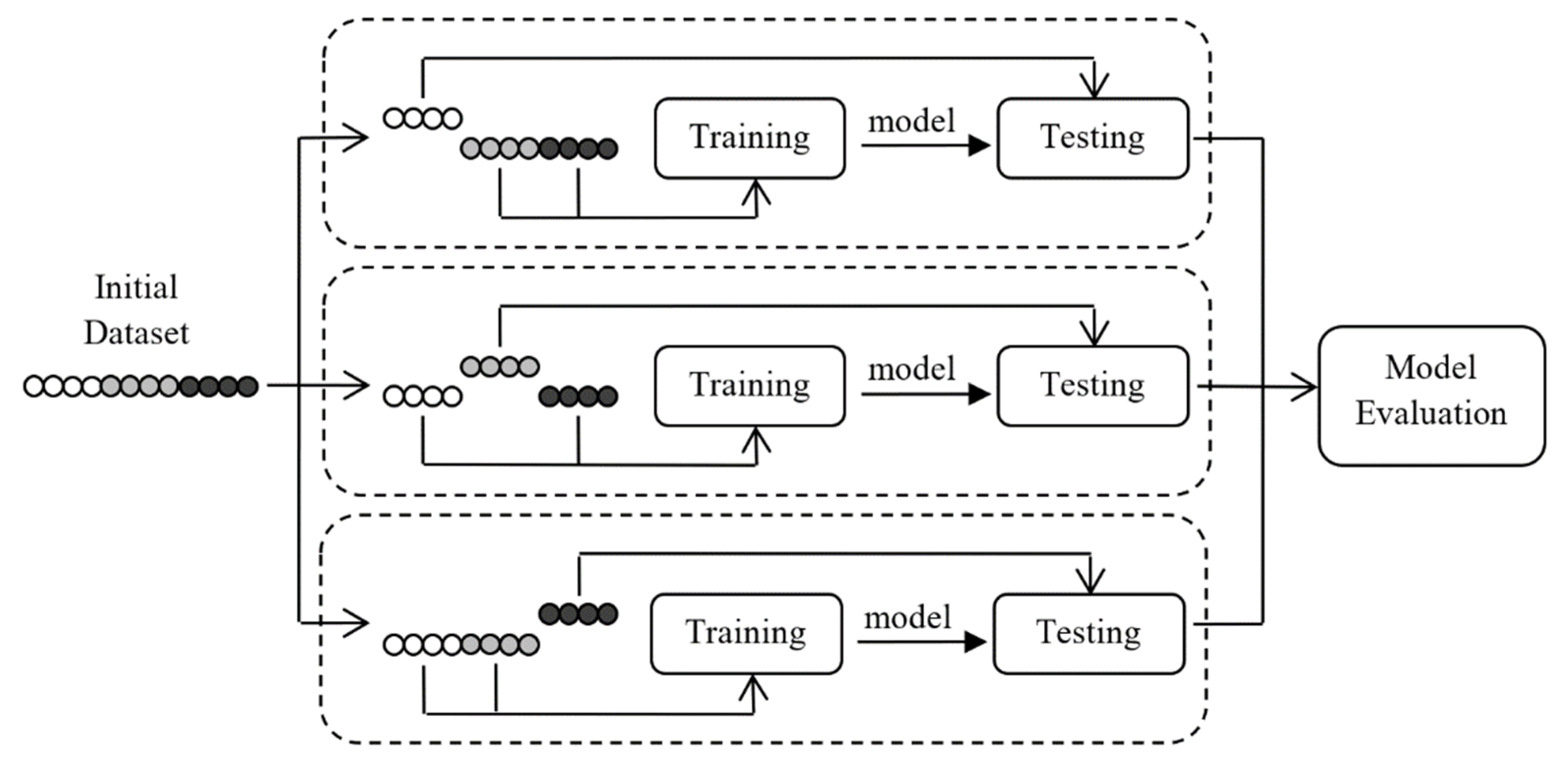
3. Methodology
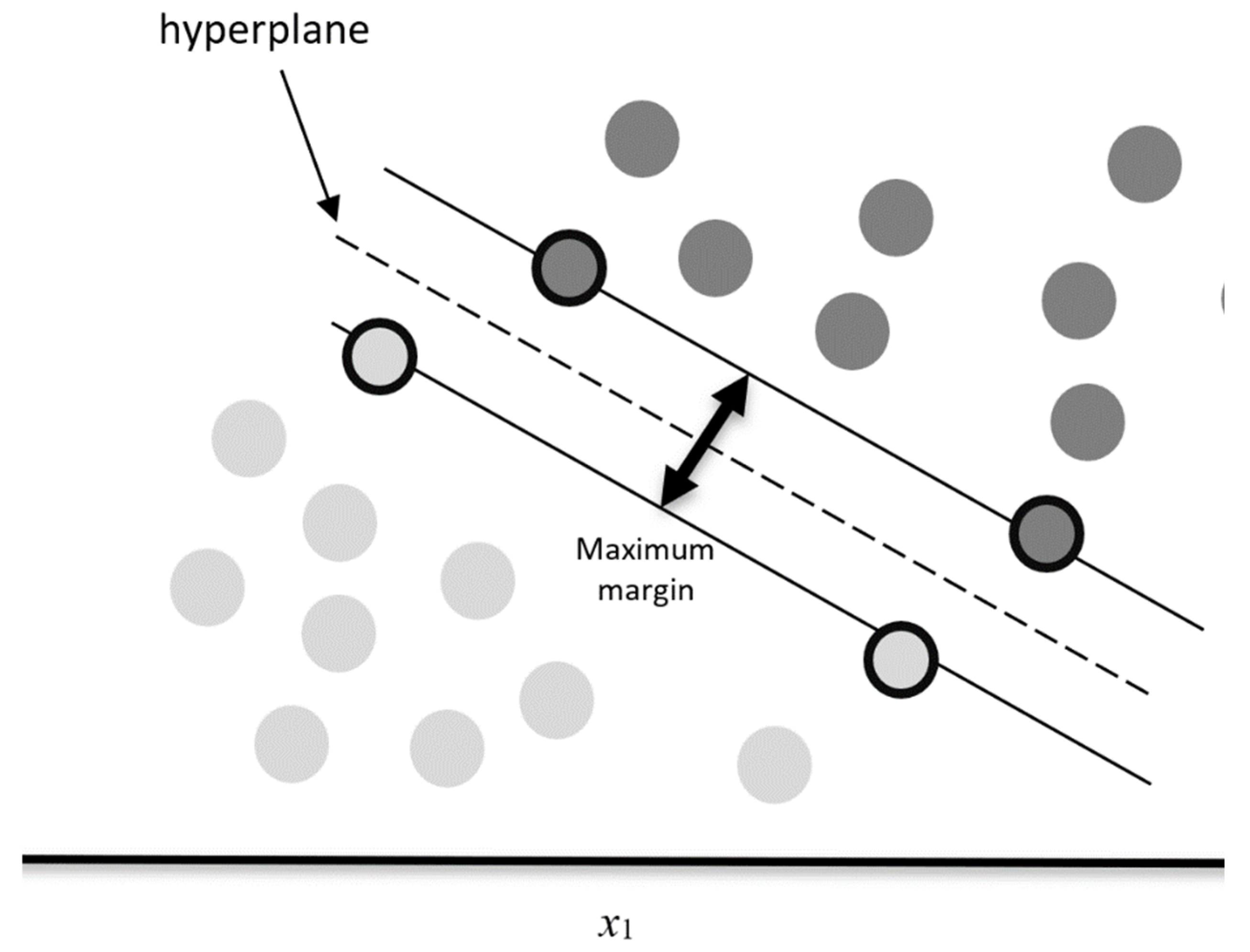
3.1. Support Vector Machines
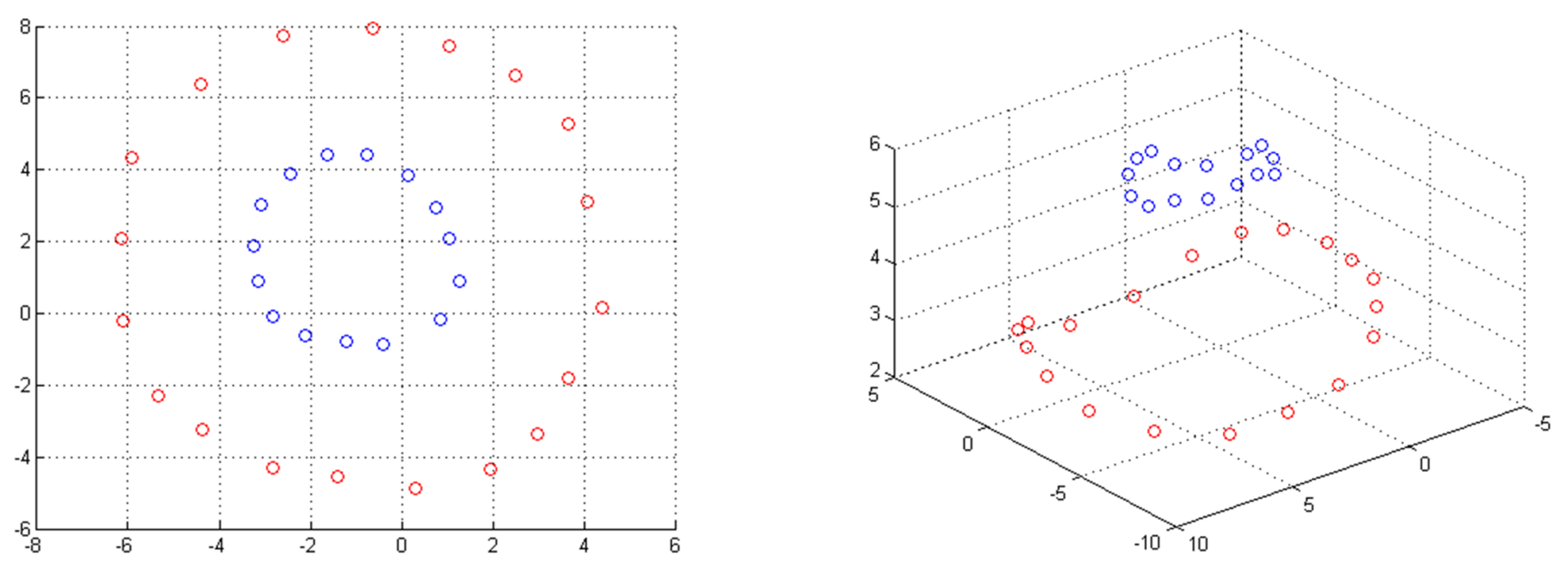
3.1.1. Kernel Methods
3.1.2. Over-Fitting
3.1.3. Weights
3.2. Random Forests
3.3. Performance Metrics
3.4. Empirical Results
3.4.1. SVM Models
3.4.2. Random Forest Models
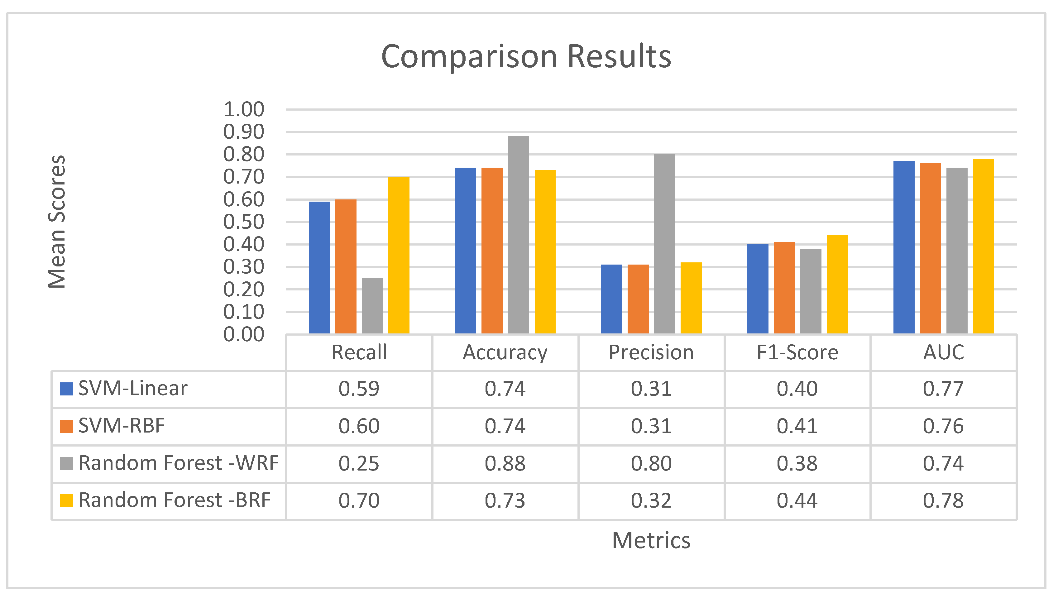
3.4.3. Comparative Results
4. Conclusions and Future Work
Author Contributions
Funding
Institutional Review Board Statement
Informed Consent Statement
Data Availability Statement
Conflicts of Interest
References
- OECD. Health at a Glance 2019: OECD Indicators; OECD Publishing: Paris, France, 2019. [Google Scholar] [CrossRef]
- Cardiff, K.; Anderson, G.; Sheps, S. Evaluation of a Hospital-Based Utilization Management Program. Healthc. Manag. Forum 1995, 8, 38–45. [Google Scholar] [CrossRef]
- Ashton, C.M.; Wray, N.P. A conceptual framework for the study of early readmission as an indicator of quality of care. Soc. Sci. Med. 1996, 43, 1533–1541. [Google Scholar] [CrossRef]
- Zhao, P.; Yoo, I.; Naqvi, S.H. Early Prediction of Unplanned 30-Day Hospital Readmission: Model Development and Retrospective Data Analysis. JMIR Med. Inform. 2021, 9, e16306. [Google Scholar] [CrossRef] [PubMed]
- Anderson, G.F.; Steinberg, E.P. Predicting hospital readmissions in the Medicare population. Inq. J. Med. Care Organ. Provis. Financ. 1985, 22, 251–258. [Google Scholar]
- Tabak, Y.P.; Sun, X.; Nunez, C.M.; Gupta, V.; Johannes, R.S. Predicting Readmission at Early Hospitalization Using Electronic Clinical Data. Med. Care 2017, 55, 267–275. [Google Scholar] [CrossRef] [Green Version]
- Kelly, J.F.; McDowell, H.; Crawford, V.; Stout, R.W. Readmissions to a geriatric medical unit: Is prevention possible? Aging Clin. Exp. Res. 1992, 4, 61–67. [Google Scholar] [CrossRef]
- Jencks, S.F.; Williams, M.V.; Coleman, E.A. Rehospitalizations among Patients in the Medicare Fee-for-Service Program. N. Engl. J. Med. 2009, 360, 1418–1428. [Google Scholar] [CrossRef]
- Ashton, C.M.; Del Junco, D.J.; Souchek, J.; Wray, N.P.; Mansyur, C.L. The Association between the Quality of Inpatient Care and Early Readmission. Med. Care 1997, 35, 1044–1059. [Google Scholar] [CrossRef]
- Benbassat, J.; Taragin, M. Hospital Readmissions as a Measure of Quality of Health Care. Arch. Intern. Med. 2000, 160, 1074–1081. [Google Scholar] [CrossRef]
- Fischer, C.; Lingsma, H.; Marang-van de Mheen, P.J.; Kringos, D.S.; Klazinga, N.S.; Steyerberg, E.W. Is the Readmission Rate a Valid Quality Indicator? A Review of the Evidence. PLoS ONE 2014, 9, e112282. [Google Scholar] [CrossRef] [Green Version]
- Wang, H.; Cui, Z.; Chen, Y.; Avidan, M.; Ben Abdallah, A.; Kronzer, A. Predicting Hospital Readmission via Cost-Sensitive Deep Learning. IEEE/ACM Trans. Comput. Biol. Bioinform. 2018, 15, 1968–1978. [Google Scholar] [CrossRef] [PubMed]
- Kansagara, D.; Englander, H.; Salanitro, A.; Kagen, D.; Theobald, C.; Freeman, M.; Kripalani, S. Risk Prediction Models for Hospital Readmission. JAMA 2011, 306, 1688–1698. [Google Scholar] [CrossRef] [PubMed] [Green Version]
- Zhou, H.; Della, P.R.; Roberts, P.; Goh, L.; Dhaliwal, S.S. Utility of models to predict 28-day or 30-day unplanned hospital readmissions: An updated systematic review. BMJ Open 2016, 6, e011060. [Google Scholar] [CrossRef] [PubMed]
- Li, Q.; Yao, X.; Échevin, D. How Good Is Machine Learning in Predicting All-Cause 30-Day Hospital Readmission? Evidence From Administrative Data. Value Health 2020, 23, 1307–1315. [Google Scholar] [CrossRef]
- Futoma, J.; Morris, J.; Lucas, J. A comparison of models for predicting early hospital readmissions. J. Biomed. Inform. 2015, 56, 229–238. [Google Scholar] [CrossRef] [Green Version]
- Zhou, J.; Li, X.; Wang, X.; Chai, Y.; Zhang, Q. Locally weighted factorization machine with fuzzy partition for elderly readmission prediction. Knowl.-Based Syst. 2022, 242, 108326. [Google Scholar] [CrossRef]
- Mahmoudi, E.; Kamdar, N.; Kim, N.; Gonzales, G.; Singh, K.; Waljee, A.K. Use of electronic medical records in development and validation of risk prediction models of hospital readmission: Systematic review. BMJ 2020, 369, m958. [Google Scholar] [CrossRef] [Green Version]
- Huang, Y.; Talwar, A.; Chatterjee, S.; Aparasu, R.R. Application of machine learning in predicting hospital readmissions: A scoping review of the literature. BMC Med. Res. Methodol. 2021, 21, 96. [Google Scholar] [CrossRef]
- Pitoglou, S.; Koumpouros, Y.; Anastasiou, A. Using Electronic Health Records and Machine Learning to Make Medical-Related Predictions from Non-Medical Data. In Proceedings of the 2018 International Conference on Machine Learning and Data Engineering (iCMLDE), Sydney, Australia, 3–7 December 2018; pp. 56–60. [Google Scholar] [CrossRef]
- Du, G.; Zhang, J.; Luo, Z.; Ma, F.; Ma, L.; Li, S. Joint imbalanced classification and feature selection for hospital readmissions. Knowl.-Based Syst. 2020, 200, 106020. [Google Scholar] [CrossRef]
- Du, G.; Zhang, J.; Ma, F.; Zhao, M.; Lin, Y.; Li, S. Towards graph-based class-imbalance learning for hospital readmission. Expert Syst. Appl. 2021, 176, 114791. [Google Scholar] [CrossRef]
- Cortes, C.; Vapnik, V. Support-vector networks. Mach. Learn. 1995, 20, 273–297. [Google Scholar] [CrossRef]
- Breiman, L. Bagging predictors. Mach. Learn. 1996, 24, 123–140. [Google Scholar] [CrossRef] [Green Version]
- Albacete, F.J.V.; Peláez-Moreno, C. 100% Classification Accuracy Considered Harmful: The Normalized Information Transfer Factor Explains the Accuracy Paradox. PLoS ONE 2014, 9, e84217. [Google Scholar] [CrossRef] [Green Version]

| No | Independent Variables | Characterization of Each Variable |
|---|---|---|
| Panel A: General Information/Patient Data | ||
| 1 | Patient Age | Quantitative variable, Integer |
| 2 | Patient Gender | Qualitative variable, Categorical |
| 3 | Length of Stay | Quantitative variable, Integer |
| 4 | Patient Transfer | Qualitative variable, Binary |
| 5 | ICD-10 Diagnosis on Admission | Qualitative variable, Categorical |
| 6 | ICD-10 Diagnosis at Discharge | Qualitative variable, Categorical |
| 7 | Admission Clinic | Qualitative variable, Categorical |
| 8 | Discharge Clinic | Qualitative variable, Categorical |
| 9 | Clinic Change | Qualitative variable, Binary |
| 10 | Hospitalization Outcome | Qualitative variable, Categorical |
| 11 | Past Hospitalization | Qualitative variable, Binary |
| Panel B: Operational Status of the Clinic | ||
| 12 | Clinic’s Occupancy Rate | Quantitative variable, Continuous |
| 13 | Clinic’s Number of Doctors | Quantitative variable, Integer |
| 14 | Clinic’s Number of Nurses | Quantitative variable, Integer |
| Panel C: Laboratory results | ||
| 15 | Blood Sugar (Glucose) | Quantitative variable, Continuous |
| 16 | Indication (Normal Range) Blood Sugar | Qualitative variable, Categorical |
| 17 | Potassium | Quantitative variable, Continuous |
| 18 | Indication (Normal Range) Potassium | Qualitative variable, Categorical |
| 19 | Sodium | Quantitative variable, Continuous |
| 20 | Indication (Normal Range) Sodium | Qualitative variable, Categorical |
| 21 | Blood Urea Nitrogen | Quantitative variable, Continuous |
| 22 | Indication Blood Urea (Normal Range) Nitrogen | Qualitative variable, Categorical |
| 23 | Blood Creatinine | Quantitative variable, Continuous |
| 24 | Indication (Normal Range) Blood Creatinine | Qualitative variable, Categorical |
| Predicted | |||
|---|---|---|---|
| 0 | 1 | ||
| Actual | 0 | TN (True Negatives) | FP (False Positives) |
| 1 | FN (False Negatives) | TP (True Positives) | |
| Parameter C | Parameter γ | |
|---|---|---|
| SVM Linear Kernel | 0.06 | --- |
| SVM RBF Kernel | 194.38 | 0.0001 |
| Confusion Matrix (SVM, Linear Kernel) | |||
|---|---|---|---|
| Predicted | |||
| 0 | 1 | ||
| Actual | 0 | TN 732 | FP 220 |
| 1 | FN 68 | TP 98 | |
| Confusion Matrix (SVM, RBF Kernel) | |||
|---|---|---|---|
| Predicted | |||
| 0 | 1 | ||
| Actual | 0 | TN 730 | FP 222 |
| 1 | FN 67 | TP 99 | |
| SVM Linear Kernel | ||||
| Recall | Accuracy | Precision | F1-Score | AUC |
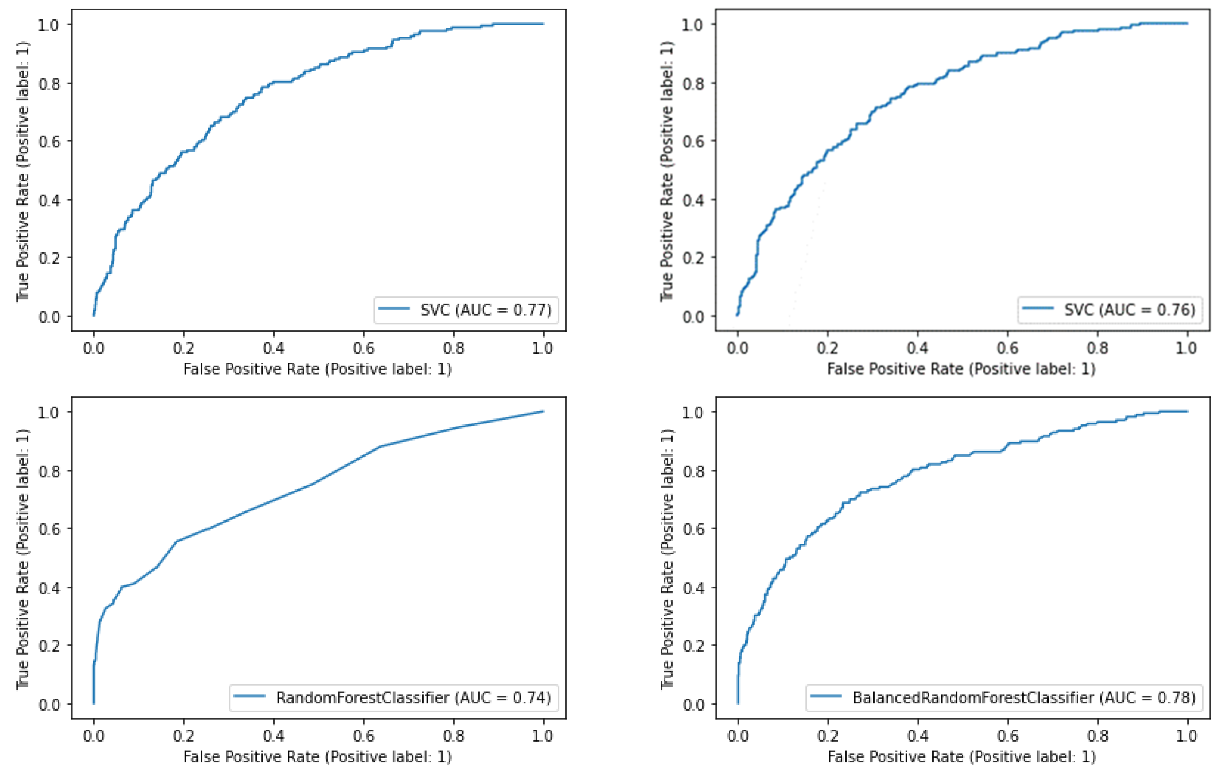
| 0.59 | 0.74 | 0.31 | 0.40 | 0.77 |
| SVM RBF Kernel | ||||
| Recall | Accuracy | Precision | F1-Score | AUC |
| 0.60 | 0.74 | 0.31 | 0.41 | 0.76 |
| Total Number of Decision Trees | |
|---|---|
| Weighted Random Forest | 25 |
| Balanced Random Forest | 730 |
| Confusion Matrix (Weighted Random Forest) | |||
|---|---|---|---|
| Predicted | |||
| 0 | 1 | ||
| Actual | 0 | TN 942 | FP 10 |
| 1 | FN 125 | TP 41 | |
| Confusion Matrix (Balanced Random Forest) | |||
|---|---|---|---|
| Predicted | |||
| 0 | 1 | ||
| Actual | 0 | TN 704 | FP 248 |
| 1 | FN 50 | TP 116 | |
| Weighted Random Forest | |||||
| Recall | Specificity | Accuracy | Precision | F1-Score | AUC |
| 0.25 | 0.98 | 0.88 | 0.80 | 0.38 | 0.74 |
| Balanced Random Forest | |||||
| Recall | Specificity | Accuracy | Precision | F1-Score | AUC |
| 0.70 | 0.74 | 0.73 | 0.32 | 0.44 | 0.78 |
| Importance | Feature |
|---|---|
| 0.141501 | ICD-10 Diagnosis at Discharge |
| 0.129996 | ICD-10 Diagnosis on Admission |
| 0.059492 | Clinic’s Occupancy Rate |
| 0.056195 | Hospitalization Outcome |
| 0.05464 | Blood Urea Nitrogen |
| 0.054075 | Patient Age |
| 0.052316 | Potassium |
| 0.051854 | Blood Sugar (Glucose) |
| 0.048263 | Length of Stay |
| 0.043971 | Blood Creatinine |
| 0.042001 | Sodium |
| 0.030861 | Discharge Clinic |
| 0.03023 | Clinic’s Number of Doctors |
| 0.029398 | Clinic’s Number of Nurses |
| 0.024448 | Indication (Normal Range) Blood Sugar |
| 0.020731 | Admission Clinic |
| 0.020721 | Patient Gender |
| 0.020681 | Past Hospitalization |
| 0.019997 | Indication (Normal Range) Blood Creatinine |
| 0.019523 | Indication (Normal Range) Potassium |
| 0.016082 | Indication Blood Urea (Normal Range) Nitrogen |
| 0.01222 | Patient Transfer |
| 0.01015 | Indication (Normal Range) Sodium |
| 0.00112 | Clinic Change |
Publisher’s Note: MDPI stays neutral with regard to jurisdictional claims in published maps and institutional affiliations. |
© 2022 by the authors. Licensee MDPI, Basel, Switzerland. This article is an open access article distributed under the terms and conditions of the Creative Commons Attribution (CC BY) license (https://creativecommons.org/licenses/by/4.0/).
Share and Cite
Michailidis, P.; Dimitriadou, A.; Papadimitriou, T.; Gogas, P. Forecasting Hospital Readmissions with Machine Learning. Healthcare 2022, 10, 981. https://doi.org/10.3390/healthcare10060981
Michailidis P, Dimitriadou A, Papadimitriou T, Gogas P. Forecasting Hospital Readmissions with Machine Learning. Healthcare. 2022; 10(6):981. https://doi.org/10.3390/healthcare10060981
Chicago/Turabian StyleMichailidis, Panagiotis, Athanasia Dimitriadou, Theophilos Papadimitriou, and Periklis Gogas. 2022. "Forecasting Hospital Readmissions with Machine Learning" Healthcare 10, no. 6: 981. https://doi.org/10.3390/healthcare10060981
APA StyleMichailidis, P., Dimitriadou, A., Papadimitriou, T., & Gogas, P. (2022). Forecasting Hospital Readmissions with Machine Learning. Healthcare, 10(6), 981. https://doi.org/10.3390/healthcare10060981