Abstract
The purpose of this paper is to examine the various structural determinants of revenue and tax effort in Tunisia. We used on the empirical study an ARDL model to estimate the dynamic equation of fiscal potential and its structural and non-structural determinants covering the period of 1996–2017 in Tunisia. The empirical results show that before 2010, Tunisia fully exploited its fiscal potential, and the tax effort was above unity. After 2010 this trend was reversed. Despite the increase in the tax burden, Tunisia is below potential. The results showed that Tunisia is facing dramatic difficulties in mobilizing more tax revenue with this same taxpayer base. As a result, it is called upon to orient reform actions towards two aspects: broadening the taxpayer base to guarantee more tax fairness and adopting an awareness and motivation strategy aimed at greater tax compliance. Tunisia should adopt reforms that aim to eliminate the flat-rate regime and put in place advantages and procedures to facilitate and motivate the transition from informal to formal. Finally, it would be wise to further regulate cash payments and ensure the application of the legal rules governing the matter. In order to optimize the allocation of budgetary resources and ease the pressure on public finances, it would be appropriate, even with a delay in relation to the legislation to fight tax evasion and fraud by improving the human and material resources made available to the tax administration and consolidating its digitalization efforts.
1. Introduction
The authority or the government as manager of public finances plays a crucial role in the economic and social order of the country. Public finance allows the State to function by facing the various expenses such as: the defense of the territory, the security of citizens, education, health, infrastructure, administrative services, etc. With an essentially fiscal budget, the mobilization of fiscal resources is essential for the creation of sustained economic growth under the constraint of not compromising the economy’s capacity to create wealth within the meaning of the Laffer curve. According to Laffer (2004) “too much tax kills tax” (Laffer 2004).
Taxation is one of the main components of the tax space of countries. Its internal origin defines the relationship between government and population and makes it a key element in the mobilization of public resources. Among these countries is Tunisia, where 87% of the State’s ordinary resources are made up of tax revenues.
Governments choose a combination of taxes that allows them to obtain a sufficient level of income. We cite corporate tax, personal income tax, value added tax (VAT), excise duties, etc. It should be noted that the generation of tax revenues is a fundamental issue for the mobilization of domestic resources to finance public expenditure. As a result, fiscal performance is a matter of major priority importance to be taken into consideration in both developed and developing economies.
Benevolent governments always seek the combination that generates less distortion while ensuring sufficient revenue. With this recognition, the issue of fiscal performance is much more important for countries with low natural resources such as Tunisia. This problematic question appeals to fundamental notions, namely that the mobilization of resources is therefore taxation. The tax effort on the one hand and redistribution on the other is therefore social equity and the ability to pay on the other.
In addition, poor performance and insufficient tax revenue, either excess pressure accompanied by a structural deficit in the financing of public expenditure, means that countries have limits in their tax collection mechanisms. In this regard, these limits can be summed up in two cases. The first is the low capacity to generate tax revenue below the maximum capacity. The second is the misuse of the resources collected, in a situation of maximum fiscal capacity, to finance public investments that should normally generate more revenue.
To get around these shortcomings, particularly in countries with a high fiscal deficit and making maximum use of its taxing capacity, the fiscal deficit must be reduced through the rationalization of spending. However, if a country operates below its tax capacity, the country should undertake tax reforms that increase tax revenues to reduce the budget deficit through more productive investment.
Where is Tunisia located, that it experienced an unprecedented worsening of its budget deficit? What about fiscal capacity. In other words, is Tunisia below or below this maximum capacity?
In this context fits this study, the objective of which is to seek answers to such a question based on an estimate of the maximum tax collection capacity at the macro scale which requires knowledge of the structural determinants and non-structural tax effort.
This study will be organized as follows: firstly, we seek to present a review of the literature relating to the various structural determinants of revenue and tax effort. Secondly, our study will consist in estimating the fiscal potential of Tunisia to be able to compare the theoretical potential fiscal capacity with that observed.
2. Literature Review
Tax effort is defined as the degree to which a country’s fiscal potential is exploited. Fenochietto and Pessino (2013) present fiscal potential or contributory capacity as the maximum tax revenue that a given country can collect given structural economic, social, institutional and demographic factors (Fenochietto and Pessino 2013).
Moreover, a country’s tax effort is a one-off measure of the performance of tax resource mobilization compared to its potential. It is calculated by comparing current tax revenue to estimated tax revenue. A level greater than 1 indicates that the country in question is having difficulty mobilizing additional fiscal resources in view of the full exploitation of the potential. If the tax effort is less than 1, the country is in the case of an under exploitation of its fiscal potential and in this case the public authorities are endowed with a margin making it possible to strengthen the State’s revenue by mobilizing fiscal resources (Brun et al. 2006).
The level of tax revenue varies from country to country. It is well known that the level of development is correlated with the fiscal performance of countries. This difference means that the evaluation of tax revenues and the analysis of their determinants pose methodological problems. Such difficulties arise from the fact that tax revenues are closely linked on the one hand to economic policy choices, and on the other hand they are the result of the evolution of a set of structural factors characterizing the countries. To get around these difficulties, the solution proposed by Stotsky and WoldeMariam (1997) consists in calculating the fiscal effort with the decomposition in the effect of economic policy and the effect of structural factors (Stotsky and WoldeMariam 1997).
Beyond the complexity of measurement, another major difficulty has been added—in this case, the question of the instability of these recipes (Guillaumont 1987; Araujo et al. 1999; Stampini et al. 2013). This instability of revenue is itself due to the complexity of the set of factors that are difficult to control by the policies that determine it, in particular the prices of basic products (Dawe 1996; Brun et al. 2011; Collier and Gunning 1999). In addition, the instability of revenues may be linked to the legal definition of the base such as the case of certain consumption taxes in many developing countries. In fact, in these countries, and for reasons considered to be social, basic goods whose consumption is the most stable are frequently exempt from consumption taxes. As confirmed by Brun et al. (2006) the tax then sits on the unstable part of the plate. One solution to these problems of instability in macroeconomic analyses has generally been to resort to deterministic trend models (Lardic and Mignon 2002).
It should therefore be noted that the subject of the tax effort and the analysis of its determinants aroused the interest of several economists and specialists in public finance. This subject remains problematic for all developed and developing economies. Several works followed one another, especially in the late sixties until the end of the millennium with the study of Stotsky and WoldeMariam (1997).
Hinrichs (1965) was the pioneer who became interested in the subject. He tried to determine public revenues, tax and non-tax, for a panel of 60 countries observed over the period of 1957–1960, using as explanatory variables “income per capita” and “openness of the economy”, with exports related to GNP. He showed that for countries with a per capita income of less than $500, openness is a better estimator of government revenue (Hinrichs 1965).
In fact, it should be noted that most studies on the determinants of the tax effort are based essentially on econometric approaches.
Through the analysis of the determinants of the fiscal effort in sixteen Arab countries for the period of 1994–2000, Eltony (2002) concluded that the fiscal pressure is impacted in a significant and negative way by the share of mines, positively by per capita income for the six Arab countries of the Gulf Cooperation Council (GCC). As for the other non-oil producing countries, the results were statistically significant with a negative effect on the share of agriculture while the effect was rather positive for the share of mines, the share of imports, the share of exports and per capita income (Eltony 2002).
There are many studies on fiscal potential, especially for developing countries (Bahl 1971; Tanzi et al. 1987; Leuthold 1991; Stotsky and WoldeMariam 1997). However, little research has examined the quality of institutions as a determinant of tax collection and potential. In addition to the classic determinants of tax revenue, the quality of institutions and governance are important factors explaining the low collection of taxes in many countries. Indeed, these factors can affect tax revenues as they are the implicit sources of tax evasion, inappropriate exemptions and the emergence of weak tax administration (Tanzi and Davoodi 2000).
Cyan et al. (2013) highlighted the economic logic underlying the concept of the tax effort as defined in previous studies and attempted to link the tax effort to the financing needs of each country. Their study was based on a sample of 94 countries over the period of 1970–2009 to compare the two approaches used to determine the tax effort of countries, traditional regression approach by adding institutional factors and two-step stochastic frontier approach, a new approach consisting in determining the fiscal effort of countries in accordance with their public expenditure. They concluded that a country’s level of public spending can be used as additional information to quantify its tax effort (Cyan et al. 2013).
In addition, several studies have shown that tax administrations are the most subject and the most affected by corruption and bad governance. Such a result is confirmed by the studies of Bird (2004) and by (Alm and Martinez-Vazquez 2003). This suggests that a successful tax reform should be anchored in a strong political will and that the fiscal situation of a country reflects its political or “societal” institutions (Bird et al. 2008). Indeed, Bird et al. (2008) conclude that a state must guarantee the rule of law and control corruption to ensure a precondition for better tax collection. In the same direction, Botlhole (2010) has shown that the fiscal effort of a country could be influenced by its institutional factors such as corruption and the quality of regulation (Botlhole 2010).
Langford and Ohlenburg (2016) have used the stochastic frontier model of Battese and Coelli (1995) to study fiscal capacity in 85 resource-poor countries over a 27-year period. They added the ECI Economic Complexity Index, ethnic tensions and credit to the private sector to traditional determinants of fiscal capacity (Langford and Ohlenburg 2016; Battese and Coelli 1995).
Fenochietto and Pessino (2013) based on the work of Aigner et al. (1977) and (Alfirman 2003) have used a stochastic frontier model to determine the tax effort of 96 countries during the period of 1991–2006. The results show the existence of a positive and significant impact of per capita income and the opening rate and public expenditure on education as a percentage of GDP on the tax burden. Inflation (the growth rate of the consumer price index), the distribution of income as measured by the GINI index, the share of agriculture in GDP and corruption tend to decrease the tax burden significantly (Aigner et al. 1977).
Gupta (2007), through a regression on panel data for a period of 25 years covering 105 developing countries, showed that the structural factors, namely income per capita, the share of agriculture in GDP and openness, measured by the share of imports in GDP as well as foreign aid, significantly determine the performance of public revenue. Other institutional factors measured by the degree of corruption and political stability significantly influence tax revenues in developing countries. Indeed, for low- and middle-income countries, corruption negatively affects public revenue. Political stability positively influences revenue collection for low-income countries (Gupta 2007).
In summary, the review of the empirical and theoretical literature presented so far leads to a list of variables in Table 1 that determine the tax burden and which can be grouped into two broad classes in accordance with the dimension’s structural variables and institutional variables.

Table 1.
Variables determinant the tax burden.
3. Research Methodology
To estimate the tax effort amounts to estimating the theoretical tax potential to compare it to the actual tax revenue. From this it is necessary to mobilize certain structural factors making it possible to define the level of revenue that a country can collect to predict the maximum level of income that the country can generate considering its characteristics, structural and institutional.
At this level, we must distinguish between the fiscal performance of a country which is linked to its ability to collect taxes and the fiscal potential which depends on structural and non-structural characteristics. However, this distinction is very fine when it comes to estimating the tax effort. Indeed, the latter is influenced by all structural and institutional aspects. Thus, tax performance can be influenced by political decisions regarding the adoption of tax laws, tax management, the efficiency of tax collectors, tax collection, quality of institutions, quality of bureaucracy and corruption. It is therefore by improving its performance that a country can reach its fiscal potential or its fiscal capacity. To remain consistent with these theoretical and empirical suggestions and due to the unavailability of data relating to the institutional dimension, we will proceed in this work to the assessment of the tax potential and therefore of the tax effort based on structural variables and some institutional variables.
4. Evolution of the Structure of Tax Revenues in Tunisia
During the 1986–2018 study period, Tunisia’s fiscal pressure went through three phases presented in Figure 1:
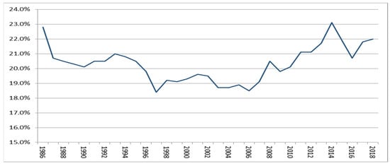
Figure 1.
Evolution of the tax pressure in Tunisia between 1986 and 2018 in % of GDP. Source: Ministry of Finance in Tunisia, 2019.
- -
- The first period, 1986–1991, returned to the crisis of the 1980s and the adoption of the Structural adjustment plan in 1986 and the change of the political regime in 1987 during which the fiscal pressure reached a level of 22.8%.
- -
- The second period 1992–2007 is marked by a decrease to a level of 18.4% in 1997. This period is marked by political stability and a resumption of economic growth.
- -
- The third period 2008–2018 was characterized by an upward trend which heralds the onset of political regime problems which accelerated during the transition period. Over the entire study period, the average tax pressure was around 20.3% of GDP. However, this rate touched the unprecedented level of 23.1% in 2014, exceeding the 22.8% recorded during the period of the crisis of the eighties. So, in this context, is Tunisia still capable of draining more fiscal resources?
Tunisia’s tax revenue structure presented in Figure 2, Figure 3 and Figure 4 below, has undergone a change since the 1990s. Indeed, the weight of indirect taxes has continued to decrease compared to direct taxes. This change can be explained by the improvement in the competitiveness of Tunisian companies on the one hand and the acceleration of the process of opening to the outside world. For the post-revolution period the increase in the share of direct taxes is due to wage increases which contributed to the increase in the tax base.
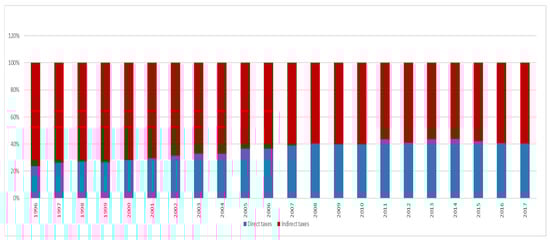
Figure 2.
Evolution of the Tax Revenue structure in Tunisia between 1996 and 2017. Source: Ministry of Finance in Tunisia, 2019.
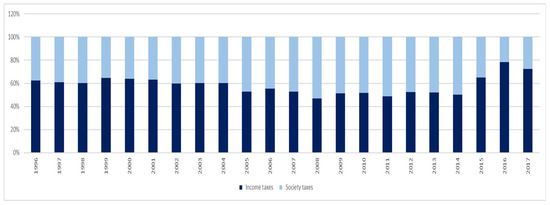
Figure 3.
Evolution of the Direct taxes structure in Tunisia between 1996 and 2017. Source: Ministry of Finance in Tunisia, 2019.
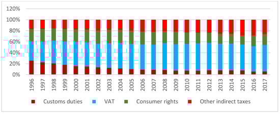
Figure 4.
Evolution of the Indirect taxes structure in Tunisia between 1996 and 2017. Source: Ministry of Finance in Tunisia, 2019.
5. Model Design and Research Methods
The estimate of the fiscal effort is based on researching the determinants of the country’s fiscal capacity. Therefore, the tax effort will undoubtedly be determined by the main factors that can explain the mobilization of resources and the creation of wealth. More precisely, the main conditions for the creation of national wealth are those such as government policies, the structure of the economy, institutions, the stage of development, etc. From these findings, we can adopt that the relationship between the tax effort and the capacity to create wealth are theoretical evidence. As a result, the work relating to the subject is mainly interested in the empirical validation and research of the fundamental determinants that show differences between countries and tax systems.
Based on the study presented above, the objective of predicting the maximum level of income that the country can generate or the estimation of an equation of fiscal potential must consider the structural factors making it possible to define the level of income that a country can collect.
Even if the tax potential differs from the tax performance, which can be influenced by political decisions regarding the adoption of tax laws, tax management, the level of training of tax collectors, the quality of institutions, quality of bureaucracy and corruption. In this study, we will adopt that improving fiscal performance is the same condition for a country to achieve its fiscal potential or fiscal capacity.
In this article we will remain consistent with this point of view, the assessment of the fiscal potential which will bring us back to the estimation of the fiscal effort that will be based on structural variables, namely the GDP per capita (GDPh), which reflects the level of development and therefore the national income which constitutes the tax base. In addition, the demand for public goods increases with the level of development (Wagner’s law). The share of agriculture in added value (Agri) is an important factor in determining tax revenue. Indeed, for most developing countries, the agricultural sector is either exempt or is difficult to tax. A higher share of the non-agricultural sector in GDP should therefore produce a higher tax ratio (Bird et al. 2008).
Openness (Open) apprehended by the sum of exports and imports in relation to GDP. As Lotz and Morss (1967) indicated, taxing capacity increases with the volume of foreign trade for several reasons. It is administratively easier to tax trade flows (Lotz and Morss 1967). Openness to trade generates productivity gains and growth gains (Frankel and Romer 1999).
The demand for public services is an important factor in inducing the population to behave as taxpayers, which suggests that the presence of a large rural sector reduces tax revenue (Tanzi and Adam 1992). Therefore, to give an approximation of the demand for public services, we have included the share of the urban population (Urban).
Furthermore, it is recognized that the development of financial transactions can generate positive effects on investment and on economic growth and therefore on the tax base. In this sense, we will use the degree of monetization, apprehended by the M2 money supply over GDP (M2_GDP), which makes it possible to capture this effect on the tax levy.
In addition to the structural determinants of fiscal potential, the quality of institutions and governance have been widely discussed in the literature as important factors that explain the low collection of taxes in many countries, particularly developing countries. Indeed, these factors affect tax revenues, as they constitute the causes behind the emergence of tax evasion, inappropriate tax exemptions and weak tax administration (Tanzi and Davoodi 2000). Indeed, good governance, respect for the rule of law and control of corruption seem to be the essential preconditions for a more adequate tax collection effort (Bird et al. 2008). In this context we will use a variable for governance (Gov) which will be measured by the average of six indicators published by the World Bank of (Kaufmann et al. 2004). These six indicators include control of corruption, government efficiency, political stability and freedom from violence/terrorism, regulatory quality, rule of law and voice and accountability presented in the definition and measurement of governance. The average is calculated using the estimated scores. In fact, the estimated scores vary between −2.5 and 2.5 so that they are positive, and the scale has been transformed to 0 to 5. Thus, for the missing observations, particularly the years 1997–1999–2001, we have extrapolated the data using the average of the two years before and after. To capture the effect of the democratic transition period experienced by Tunisia since the year 2011, we will use a dummy variable (Dummy) which takes the value 0 before 2011 and the value 1 after.
Since the optimal tax revenues are not observed, we approximate the optimal tax burden by a linear combination of explanatory variables. After estimating this linear combination, we calculate the optimal tax rate and predicted values of the model that we compare with the effective tax pressure. Thus, we will estimate a linear equation of the tax pressure as a dependent variable, according to the structural and institutional determining factors as independent variables.
The model will take the following linear form:
where:
- : The effective tax pressure, tax revenue in relation to GDP.
- : The vector of explanatory variables consisting of:
- GDPh: Real GDP per capita.
- Agri: Share of added value of agriculture in GDP.
- Open: Opening rate (Export + Imports in relation to GDP).
- M2_gdp: The M2 variant of the money supply in GDP.
- Urban: Urbanism rate.
- Gov: The average of the six governance indicators of the World Bank.
- Dummy: Dummy variable .
The model to be estimated will take the following form:
where:
- C: constant
- αi: The coefficients relating to the dependent variables
6. Data Sources
The relative variable time series (GDPh, Agri, Open, Urban,) were collected from the national databases of the Tunisian National Statistics Institute (TNSI). For the tax pressure, it was based on data from the Tunisian Ministry of Finance. The M2_PIB money supply was collected from the databases of the Central Bank of Tunisia (CBT). The variable (Gov) was calculated based on the six governance indicators of the World Bank. The sample was made up of 22 annual observations covering the period of 1996–2017. The choice of the period was constrained by the availability of data on governance.
7. Stationarity and Order of the Integration of Variables
Generally, the analysis of temporal data first requires examining the stationarity of the variables to know their order of integration and level of stationarity. This study is necessary, because the use of nonstationary time series will lead to a fallacious regression (Harris and Sollis 2003; Alimi 2014). This study has the consequence that the T-statistics of the coefficients will be highly significant and that the F-statistic will not be, with a very low coefficient of determination (R2), higher than the Durbin–Watson statistic (DW) and committing a large frequency of type 1 errors (Granger and Newbold 1974). Therefore, going through the stationarity tests is an obligation for two reasons:
- -
- The first is to avoid the problem of fictitious regression.
- -
- The second is to choose the appropriate estimation techniques in accordance with the level of stationarity of the variables.
In this regard, the tests of Augmented Dickey and Fuller ADF (1979) and of Phillips and Perron (1988) have been commonly and widely used to determine the level of stationarity of variables (Cheung and Lai 1995; Phillips and Perron 1988). The analysis using unit root tests, mainly the Augmented Dickey–Fuller (ADF) test and the Phillips–Perron test (PP), applied to the level variables show in Table 2 below, that the variables are of mixed order of integration I (0) and I (1). Such a result verifies the condition necessary for the application of the cointegration technique according to the ARDL model (Auto Regressive Distributed Lag) (Pesaran et al. 2001). Which requires that the dependent variable l (pf) be integrated of order 1 I (1), and that the explanatory variables are mixed either I (1) or I (0) and that none of the variables integrated are of order 2 I (2). Therefore, the statistical characteristics of the variables provide information on the existence of a cointegration relation according to an unconstrained error-correction model of Pesaran et al. (2001) or the ARDL (Auto Regressive Distributed Lag) model. Indeed, the relation between the fiscal potential and its determinants can be a relation which tends towards a long-term equilibrium. The short term has always been characterized by adjustments that are made through interventions in annual finance laws. This is the case for Tunisia, which rectifies taxes on an annual basis either by eliminating or adding certain taxes to each finance law.
Table 2.
Stationarity and order of integration of variables.
Therefore, we use an ARDL model to estimate the dynamic equation of fiscal potential and its structural and non-structural determinants. The ARDL model is a scaled-delay autoregressive model proposed by Pesaran and Shin (1998) and Pesaran et al. (2001) makes it possible, on the one hand, to test long-term relationships using the “bounds test” on series that are not integrated of the same order and, on the other hand, to obtain better estimates on small samples (Pesaran and Shin 1998; Pesaran et al. 2001). Thus, ARDL gives the possibility of simultaneously dealing with long-term dynamics and short-term adjustment (Narayan and Smyth 2005).
Taking the general form of an ARDL, our model equation is written:
This equation can be broken down into three blocks:
- -
- The first (1) is the log term relation.
- -
- The second (2) the term cost adjustment by the “p” lags of the dependent variable LPF.
- -
- The third (3) the short-term adjustment by the “k” lags of the explanatory variables X (LGFCF, LAgri, Lgov, LM2_GDP, LOpen, LGDPh, LUrban, Dummy).
8. Empirical Results
The approach generally used to estimate an ARDL consists of the following conditions:
- -
- Estimate the model chosen according to the Akaike information criteria,
- -
- Perform the long-term relationship existence test using the Bound test.
- -
- Estimate the relation to the error-correction term.
- -
- Perform the necessary tests, serial correlation test and CUSUM stability test.
- -
- Reject or accept and interpret the model.
For the estimations, we first estimated the model using all the explanatory variables, with LPF as a function of the other variables.
The model chosen according to the SIC criterion is ARDL (1, 2, 2, 2, 2, 1) presented in Figure 5 below, with a single delay for the dependent variable lPF. For the explanatory variables: 2 delays for LGDPh, 2 delays for Lm2_GDP, 2 delays for LGov, 2 delays for LUrban and a single delay for LAgri.
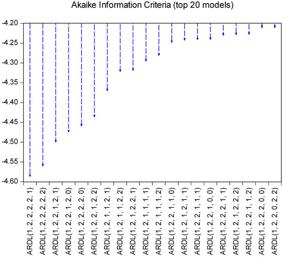
Figure 5.
Estimation of the model chosen according to the Akaike information criteria. Source: The authors.
The model chosen for the estimation is with constant and without trend. We did not use the variable Dummy and we are constrained by the number of observations.
The results of the bounds test presented in Table 3 below, show that there is a cointegration relationship between LPF and the other explanatory variables at a level of 2.5% (F-statistic is of the order of 3.96, which is greater than the sup band I (I) = 3.73).
Table 3.
The results of the Estimation of the model ARDL Long Run Form and Bound test.
The results presented in Table 3, also show that for the long-term relationship, except for LM2_GDP, the log of the money supply in GDP, the other explanatory variables are not significant.
The results presented in Table 4, Table 5 and Table 6 and Figure 6 and Figure 7, showed that although the “Breusch–Godfrey Serial Correlation LM Test” showed no serial correlation, the CUSUM Cumulative Sum test shows that the model is not stable. We cannot accept the model with this shape.
Table 4.
The results of the estimation of the model with the error-correction term (ECT).
Table 5.
The results of the Breusch–Godfrey Serial Correlation LM test.
Table 6.
The results of the Ramsey RESET test.
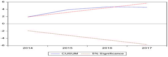
Figure 6.
Results of CUSUM stability test. Source: The authors.
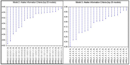
Figure 7.
Results of CUSUM stability test. Source: The authors.
The results of the long-term relationship show that for the two variables LUrban and LAgri, the coefficients are not statistically significant. However, agricultural activity is inversely related to the level of urban planning, so the existence of two variables in the same equation may affect the results.
Therefore, we estimated two models using the LUrbain variable first and the LAgri variable second.
The ARDL Bound test output presented in this Table 7 indicates that for both models the results confirm the existence of a long-term relationship between the variables for the period considered. Indeed, the calculated F-statistic was greater than the critical values greater than the significance level of 1% for model 2 and 2.5% for model 3; therefore, we can retain that there is a cointegration relationship between the series in level. It should be noted that for model 4 presented in Table 8 below, the bound test does not confirm the existence of a cointegration relation in the presence of the Lopen variable.
Table 7.
The results of the ARDL Long Run Form and Bound test (Model 2 and Model 3).
Table 8.
The results of the ARDL Long Run Form and Bound test (Model 4).
After identifying the existence of the long-term relationship, we estimated the two models with the error-correction term. The ECM result indicates that the relationship between the variables met the a priori expectations and satisfied the necessary stability condition. The ECM coefficient is statistically significant and negative.
In the same sense, the coefficient of determination (R2) shows that 80% of the variations in the tax burden can be explained by the explanatory variables either in model 2 or in model 3. In addition, the results were tested using diagnostic tests, such as the Breusch–Godfrey Serial Correlation Test, Ramsey RESET, and Recursive Residual Test for Structural Stability (CUSUM). The CUSUM plot showed that the regression equation for both models is stable since the CUSUM test statistic does not exceed the limits at a 5% significance level. The results of the short-term model estimation show that the error-correction coefficient ECM (−1) is negative and significant at 1%. The coefficient of −0.45 (−0.79 for model 3) indicates that the speed of convergence towards long-term equilibrium is 45% per year (79% for model 3).
In line with the purpose of this study, we proceed to the interpretation of the results of the estimation of two models: model 2 and model 3. The real GDP per capita used as a proxy for the development of the economy is a determinant of the fiscal pressure in Tunisia. Its sign is negative and statistically significant at 1%. This result is consistent with the results released by Teera and Hudson (2004), who studied tax pressure using a panel of 116 developed and developing countries for the period of 1975–1998, where they found a negative relationship for low-income countries and a medium but positive relationship for high-income OECD countries (Teera and Hudson 2004). Additionally, Lutfunnahar (2007), by a panel on 10 developing countries including Bangladesh, Morocco and Jordan over the period of 1991–2005, also found a negative relationship between fiscal pressure and real GDP per capita. Indeed, the more income increases, the more the economy can generate more tax revenue. This relationship is conditioned to a large extent by the efficiency of the collection system (Lutfunnahar 2007).
For Tunisia, this inverse relationship can be explained by several causes:
- -
- First, the inefficiency of the tax administration in collecting additional tax revenue following economic development. This may be due to tax regulations that are still lacking in relation to the rate of economic development recorded.
- -
- Second, there is inequitable distribution of the fruits of development among the different taxpayers, which leads to the use of fraudulent maneuvers aimed at concealing the income or profits made and therefore evading the payment of tax.
- -
- Finally, the tax advantages granted by common law or by the investment incentive code (IIC) can also explain the negative relationship between tax pressure and real GDP per capita: According to the World Bank, the tax advantages granted by Tunisia under the IIC only are estimated at 1198 MD in 2009, almost 2% of GDP.
The results presented in Table 9 and Figure 8, show the effect of the change in the share of M2 money supply in GDP on the tax burden is also positive and statistically significant at 10% for model 2 and is not significant for model 3. The degree of monetization of the economy positively influences the state’s ability to mobilize more resources. Indeed, at a moderate rate of inflation, if monetary depth increases, the more the volume of economic transactions develops, and the more taxable material is created (Ngakosso 2015).
Table 9.
The results of the ARDL Error-Correction Regression.
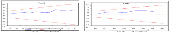
Figure 8.
Results of CUSUM tests. Source: Own study.
The degree of monetization of the economy is therefore a factor that strongly influences the public levy. According to Essid (2017), financial depth can be assessed by the ratio of the liquid liabilities of the financial system to the level of GDP, knowing that liquid liabilities are also known as broad money supply or M3. There is an upward trend in terms of the financial depth of the Tunisian banking system, going from 57% in 2001 to 70% in 2014 (Essid). This phenomenon is observed for the period of 2000–2015, favoring cash transactions, which constitutes an environment favorable to corruption, fraud and tax evasion as well as the expansion of the informal sector.
For the effect of institutional factors represented here by the governance variable, the results of model 2 show that the coefficient is statistically significant in both the short-term relationship and in the long-term relationship. Indeed, good governance is an important factor that reflects the efficiency and rationality of the tax system. Such a result largely confirms those found in empirical studies which state that inefficient institutions are the causes behind the emergence of tax evasion, inappropriate tax exemptions and weak tax administration (Tanzi and Zee 1997). Good governance, respect for the rule of law and control of corruption seem to be essential preconditions for a more adequate tax collection effort (Bird 2004).
In the long-term relationship (model 3), the share of agriculture has a negative and significant influence on the tax burden. Indeed, an increase of one point in the share of agriculture in GDP (all else equal) leads to a decrease in the tax burden of around 0.39 points for the relationship. This result is in the same direction as those of several previous studies.
Regarding the opening rate (model 2), its impact is positive but not very significant. Indeed, an increase one point in the share of imports in GDP (all else equal) leads to an increase in the tax burden of 0.42 points. Indeed, this result finds as a corollary the share of the customs regime in indirect tax revenue, which is of the order of 49% on average for the entire period. In fact, the result is expected from the fact that “income from international trade constitutes an easily taxable base than other taxes on income or on domestic consumption”. In addition, the large share of capital goods in imports may also provide an explanation for this positive relationship, as more imports of capital goods mean an increase in production and taxable wealth.
Regarding the urbanization rate, used in model 2, the results show its positive and significant effect on the tax burden in Tunisia. This conclusion confirms that found by a previous study (Torgler 2007). It seems logical that urbanization increases the demand for public goods. Consequently, the public authorities would tend to increase their effort to collect tax revenue to meet the needs of the urbanized population. In addition, it has been shown that urbanization creates an easily taxable tax base due to the concentration of formal activities in urban areas (Bird and Gendron 2007).
Based on the results of model 2, which integrates all the determinants of the tax pressure, we calculate the potential tax pressure and then the deduction of the tax effort of Tunisia during the study period in Figure 9 below.
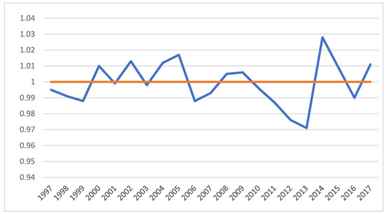
Figure 9.
Evolution of Tunisia’s Tax Effort between 1997 and 2017. Source: Ministry of Finance in Tunisia, 2019.
The results show two major trends before and after 2010. Indeed, before 2010, Tunisia fully exploited the fiscal potential. In fact, except for the year 2006 when the State benefited from a massive inflow of capital following the sale of a large part of the company Tunisia Telecom and therefore a source of revenue other than tax, the tax effort is above unity. After 2010 this trend was reversed.
These results can be explained by several factors:
- -
- For the period before 2010, the economy experienced relatively acceptable growth, characterized by its low employability, a low rate of investment and significant legal power due to the political system. That prepares the ground for a system of collection which taxes the taxpayers in an exaggerated way, especially those of the real system and the employees.
- -
- After 2010, despite the increase in fiscal pressure, Tunisia is below potential. This result can be explained by the slowdown in growth and the political situation which weakens the power of law, as well as the behavior of economic agents in matters of taxation during the post-revolution period. Indeed, in addition to tax evasion, several companies have experienced disruptions or a reduction in their activities following social movements, hence the unprecedented increase in informal activity and the unobserved economy which exceeded the equivalent of 60% of GDP.
9. Conclusions
After reviewing the results of the study, this econometric analysis shows that Tunisia is facing dramatic difficulties in mobilizing more tax revenue with this same taxpayer base. As a result, it is called upon to orient reform actions towards two major aspects: broadening the taxpayer base to guarantee more tax fairness and adopting an awareness and motivation strategy aimed at greater tax compliance. This would, through reforms that aim to eliminate the flat-rate regime and put in place advantages and procedures, facilitate and motivate the transition from informal to formal. Finally, it would be wise to further regulate cash payments and ensure the application of the legal rules governing the matter.
Since the popular uprising in Tunisia in 2011 and after the political change on 25 July 2021, Tunisia should continue to fight tax evasion and fraud by improving the human and material resources made available to the tax administration and consolidating its digitalization efforts. Additionally, it would seem one of the priorities of the government to ensure the application of the rules of good governance to improve transparency in public action. Moreover, to optimize the allocation of budgetary resources and ease the pressure on public finances, it would be appropriate, even with a delay in relation to the legislation already in force since the end of 2015, to initiate the public–private partnership to promote the quality of public services.
Concerning the fiscal policy, Tunisia should create a tax structure that will be compatible with the level of economic development, having positive effects on revenues, investments, employment and economic growth. Additionally, changes in the structure of the tax system and in the level of revenues can influence the economic activity. The higher tax rates may have a negative impact growth while lower tax rates may generate revenues that are spent in productive ways. Additionally, lowering tax rates, extending the tax basis, reducing tax exemptions and building such a tax structure can positively affect economic growth and economic development in Tunisia.
For the analysis developed in this study to test the relationship between tax effort and economic growth, we have used the ARDL model of Pesaran et al. (2001). This framework is compatible with both I(0) and I(1) series and allows the integration of short-run adjustments into the long-run equilibrium by resorting to an error-correction mechanism (ECM) through a linear transformation.
These findings open some directions for further research issues for the debate on the conduct of fiscal policy. The research in this area must analyze how increasing institutional efficiency provides greater transparency. Moreover, we can use a nonlinear ARDL (NARDL) model to analyze the long-run and short-run asymmetric effect of fiscal effort and to analyze the threshold effect relationship that may exist between economic growth and fiscal effort ((Niklas and Sadik-Zada 2019); (Sadik-Zada et al. 2021)).
Futures lines of investigation could be focused on socio-economic challenges, analyzing how the governance institutions which enhance public perceptions that the government allocates public spending fairly and may not increase tax revenue but improves administrative efficiency and fiscal capacity.
Author Contributions
Conceptualization, N.M. and I.G.; methodology, N.M. and I.G.; validation, N.M. and I.G.; investigation, N.M.; writing—original draft preparation, N.M.; writing—review and editing, N.M.; visualization, N.M. and I.G.; supervision, N.M.; project administration, N.M. All authors have read and agreed to the published version of the manuscript.
Funding
This research received no external funding.
Institutional Review Board Statement
Not applicable.
Informed Consent Statement
Not applicable.
Data Availability Statement
The data are available from the authors upon request.
Conflicts of Interest
The authors declare no conflict of interest.
References
- Aigner, Dennis, C. A. Knox Lovell, and Peter Schmidt. 1977. Formulation and estimation of stochastic frontier production function model specifications. Journal of Productivity Analysis 7: 399–415. [Google Scholar]
- Alfirman, L. 2003. Estimating Stochastic Frontier Tax Potential: Can Indonesian Local Governments Increase Tax Revenues under Decentralization? Discussion Papers in Economics, Working Paper No. 03-19. Boulder: Center for Economic Analysis, Department of Economics, University of Colorado at Boulder. [Google Scholar]
- Alm, J., and J. Martinez-Vazquez. 2003. Institutions, Paradigms, and Tax Evasion in Developing and Transition Countries. ScholarWorks, Georgia State University. Available online: https://scholarworks.gsu.edu/econ_facpub (accessed on 30 November 2021).
- Alimi, R. Santos. 2014. ARDL bounds testing approach to Cointegration: A re-examination of augmented fisher hypothesis in an open economy. Asian Journal of Economic Modelling 2: 103–14. [Google Scholar] [CrossRef]
- Araujo, Luis, Anna Dubois, and Lars-Erik Gadde. 1999. Managing interfaces with suppliers. Industrial Marketing Management 28: 497–506. [Google Scholar] [CrossRef]
- Bahl, Roy W. 1971. Measuring the creditworthiness of state and local governments: Municipal bond ratings. Presented at the Annual Conference on Taxation under the Auspices of the National Tax Association, Wednesday, September 29; pp. 64, 599–622. Available online: http://www.jstor.org/stable/23409852 (accessed on 30 November 2021).
- Battese, George Edward, and Tim J. Coelli. 1995. A model for technical inefficiency effects in a stochastic frontier production function for panel data. Empirical Economics 20: 325–32. [Google Scholar] [CrossRef] [Green Version]
- Bird, Richard, and Pierre-Pascal Gendron. 2007. The VAT in developing and transitional countries. In Cambridge Books. Cambridge: Cambridge University Press. [Google Scholar] [CrossRef]
- Bird, Richard M. 2004. Administrative dimensions of tax reform. Asia-Pacific Tax Bulletin 10: 134–50. [Google Scholar]
- Bird, Richard M., Jorge Martinez-Vazquez, and Benno Torgler. 2008. Tax effort in developing countries and high income countries: The impact of corruption, voice and accountability. Economic Analysis and Policy 38: 55–71. [Google Scholar] [CrossRef] [Green Version]
- Botlhole, T. Dineo. 2010. Tax effort and the determinants of tax ratio in sub-Saharan Africa. Presented at the International Conference on Applied Economics, Athens, Greece, August 26–28. [Google Scholar]
- Brun, Jean-François, Gérard Chambas, and Samuel Guerineau. 2011. Aide et Mobilisation Fiscale dans les Pays en Développement. Available online: https://halshs.archives-ouvertes.fr/halshs-00556804 (accessed on 30 November 2021).
- Brun, J., G. Chambas, J. Combes, P. Dulbecco, A. Gastambide, S. Guérineau, S. Guillaumont, and G. R. Graziosi. 2006. Fiscal Space in Developing Countries. Clermont-Ferrand: Center for Studies and Research on International Development (CERDI), Clermont Auvergne University, Available online: https://cerdi.uca.fr/ (accessed on 30 November 2021).
- Cheung, Yin-Wong, and Kon S. Lai. 1995. Lag order and critical values of the augmented Dickey-Fuller test. Journal of Business & Economic Statistics 13: 277–80. [Google Scholar] [CrossRef]
- Collier, Paul, and Jan Willem Gunning. 1999. Why has Africa grown slowly? Journal of Economic Perspectives 13: 3–22. [Google Scholar] [CrossRef] [Green Version]
- Cyan, Musharraf, Jorge Martinez-Vazquez, and Violeta Vulovic. 2013. Measuring Tax Effort: Does the Estimation Approach Matter and Should Effort Be Linked to Expenditure Goals? ICEPP Working Papers 39. Available online: https://scholarworks.gsu.edu/icepp/39 (accessed on 30 November 2021).
- Dawe, David. 1996. A new look at the effects of export instability on investment and growth. World Development 24: 1905–14. [Google Scholar] [CrossRef]
- Eltony, M. Nagy. 2002. Measuring Tax Effort in Arab Countries. Available online: http://erf.org.eg/wp-content/uploads/2017/05/0229-ElTony.pdf (accessed on 30 November 2021).
- Essid, Zina. 2017. Notes et Analyses de l’ITCEQ. Available online: http://www.itceq.tn/files/etudes-financieres/analyse-comparative-du-systeme-financier-tunisien.pdf (accessed on 30 November 2021).
- Fenochietto, Ricardo, and Carola Pessino. 2013. Understanding Countries’ Tax Effort. International Monetary Fund: Working Paper WP/13/244. [Google Scholar] [CrossRef]
- Frankel, Jeffrey A., and David H. Romer. 1999. Does trade cause growth? American Economic Review 89: 379–99. [Google Scholar] [CrossRef] [Green Version]
- Granger, Clive W., and Paul Newbold. 1974. Spurious regressions in econometrics. Journal of Econometrics 2: 111–20. [Google Scholar] [CrossRef] [Green Version]
- Guillaumont, Patrick. 1987. From export instability effects to international stabilization policies. World Development 15: 633–43. [Google Scholar] [CrossRef]
- Gupta, Abhijit Sen. 2007. Determinants of tax revenue efforts in developing countries. IMF Working Papers WP/07/184. [Google Scholar] [CrossRef] [Green Version]
- Harris, Richard, and Robert Sollis. 2003. Applied Time Series Modelling and Forecasting. London: Wiley. [Google Scholar]
- Hinrichs, Harley H. 1965. Determinants of government revenue shares among less-developed countries. The Economic Journal 75: 546–56. [Google Scholar] [CrossRef]
- Kaufmann, Daniel, Aart Kraay, and Massimo Mastruzzii. 2004. Governance matters III: Governance indicators for 1996, 1998, 2000, and 2002. The World Bank Economic Review 18: 253–87. [Google Scholar] [CrossRef] [Green Version]
- Laffer, Arthur B. 2004. The Laffer curve: Past, present, and future. Backgrounder 1765: 1–16. [Google Scholar]
- Langford, Ben, and Tim Ohlenburg. 2016. Tax Revenue Potential and Effort: An Empirical Investigation. Work ing Paper S 43202 UGA 1. London: International Growth Centre. [Google Scholar]
- Lardic, Sandrine, and Valérie Mignon. 2002. Econométrie des Séries Temporelles Macroéconomiques et Financières. Paris: Economica. [Google Scholar]
- Leuthold, Jane H. 1991. Tax shares in developing economies a panel study. Journal of Development Economics 35: 173–85. [Google Scholar] [CrossRef] [Green Version]
- Lotz, Joergen R., and Elliott R. Morss. 1967. Measuring “tax effort” in developing countries. Staff Papers 14: 478–99. [Google Scholar] [CrossRef]
- Lutfunnahar, Begum. 2007. A Panel Study on Tax Effort and Tax Buoyancy with Special Reference to Bangladesh. Policy Analysis Unit (PAU) Research Department, Bangladesh Bank. Working Paper Series WP 0715. Available online: www.bangladeshbank.org.bd (accessed on 30 November 2021).
- Narayan, Paresh Kumar, and Russell Smyth. 2005. The residential demand for electricity in Australia: An application of the bounds testing approach to cointegration. Energy Policy 33: 467–74. [Google Scholar] [CrossRef]
- Ngakosso, Pr Antoine. 2015. Comment la fiscalité peut-elle contribuer à la monétarisation d’une économie? Paris: Editions Publibook. [Google Scholar]
- Niklas, Britta, and Elkhan Richard Sadik-Zada. 2019. Income inequality and status symbols: The case of fine wine imports. Journal of Wine Economics 14: 365–73. [Google Scholar] [CrossRef]
- Pesaran, H. Hashem, and Yongcheol Shin. 1998. Generalized impulse response analysis in linear multivariate models. Economics Letters 58: 17–29. [Google Scholar] [CrossRef]
- Pesaran, M. Hashem, Yongcheol Shin, and Richard J. Smith. 2001. Bounds testing approaches to the analysis of level relationships. Journal of Applied Econometrics 16: 289–326. [Google Scholar] [CrossRef]
- Phillips, P., and P. Perron. 1988. Testing for a Unit Root in Time Series Regression. Biometrika 75: 335–46. [Google Scholar] [CrossRef]
- Sadik-Zada, Elkhan Richard, Wilhelm Loewenstein, and Yadulla Hasanli. 2021. Production linkages and dynamic fiscal employment effects of the extractive industries: Input-output and nonlinear ARDL analyses of Azerbaijani economy. Mineral Economics 34: 3–18. [Google Scholar] [CrossRef]
- Stampini, Marco, Ron Leung, Setou M. Diarra, and Lauréline Pla. 2013. How large is the private sector in Africa? Evidence from national accounts and labour markets. South African Journal of Economics 81: 140–65. [Google Scholar] [CrossRef]
- Stotsky, Janet Gale, and Asegedech WoldeMariam. 1997. Tax Effort in Sub-Saharan Africa. IMFWorking Paper. Washington, DC: The International Monetary Fund. [Google Scholar] [CrossRef]
- Tanzi, Mr Vito, and Antonis Adam. 1992. Fiscal Policies in Economies in Transition. Washington, DC: International Monetary Fund. [Google Scholar]
- Tanzi, Mr Vito, and Mr Hamid Reza Davoodi. 2000. Corruption, Growth, and Public Finances (Epub). Washington, DC: International Monetary Fund. [Google Scholar] [CrossRef]
- Tanzi, Vito, Mario I. Blejer, and Mario O. Teijeiro. 1987. Inflation and the measurement of fiscal deficits. Staff Papers 34: 711–38. [Google Scholar] [CrossRef]
- Tanzi, Vito, and Howell H. Zee. 1997. Fiscal policy and long-run growth. Staff Papers 44: 179–209. [Google Scholar] [CrossRef]
- Teera, Joweria M., and John Hudson. 2004. Tax performance: A comparative study. Journal of International Development 16: 785–802. [Google Scholar] [CrossRef]
- Torgler, Benno. 2007. Tax Compliance and Tax Morale: A Theoretical and Empirical Analysis. Glensanda: Edward Elgar Publishing. [Google Scholar] [CrossRef]
Publisher’s Note: MDPI stays neutral with regard to jurisdictional claims in published maps and institutional affiliations. |
© 2021 by the authors. Licensee MDPI, Basel, Switzerland. This article is an open access article distributed under the terms and conditions of the Creative Commons Attribution (CC BY) license (https://creativecommons.org/licenses/by/4.0/).