Article

Can the AD-AS Model Explain the Presence and Persistence of the Underground Economy? Evidence from Italy

Department of Social Sciences, e-Campus University, 22060 Novedrate, Italy
Economies 2021, 9(4), 170; https://doi.org/10.3390/economies9040170
Submission received: 8 October 2021 / Revised: 25 October 2021 / Accepted: 28 October 2021 / Published: 5 November 2021

Abstract

:
The underground economy crucially affects growth and unemployment in both developed and developing countries. Nevertheless, this widespread phenomenon does not appear in the basic model for macroeconomic analysis, namely the Aggregate Demand-Aggregate Supply (or simply AD-AS) model. Therefore, this paper introduces–for the first time, to the best of our knowledge–the underground sector of the economy into the popular AD-AS model, with the aim of increasing its descriptive power. Indeed, the present theoretical extension of the AD-AS model shows that the underground economy –despite its negative effects on aggregate demand and growth– can trigger a supply-side positive shock that mitigates, at least in the short run, the problem of high unemployment. Empirical evidence from Italy is also provided.

1. Introduction

The underground economy (also known as hidden economy, black economy, shadow economy and informal economy) refers to all economic activities that are hidden to tax authorities for several reasons: in particular, avoiding paying taxes and social security contributions, escaping governmental bureaucracy and regulatory burden (see, e.g., Schneider and Enste 2000, 2002). The underground economy is a widespread phenomenon around the world (albeit to varying extents) that persists over time (see, e.g., Medina and Schneider 2017, 2018). Indeed, it is a phenomenon that does not relate to only developing countries. Italy (one of the most industrialised countries) is, in fact, characterised by a high share of the underground economy.1
Furthermore, the underground economy has considerable implications on macroeconomic and fiscal performance. Specifically, two of these implications have received more attention in the literature: tax policy implications (Eng and Wong 2008; Çiçek and Elgin 2011; Frankel et al. 2013; Elgin and Uras 2013; Vegh and Vuletin 2015; Elgin and Erturk 2019; Aizenman et al. 2019; Catalina and García 2020) and implications on business cycle properties (Bajada 2003; Loayza and Rigolini 2011; Elgin 2012; Colombo et al. 2016; Abdel-Latif et al. 2017; Colombo et al. 2019; Aizenman et al. 2019; Catalina and García 2020).
Notwithstanding, the underground sector of the economy finds no place in the most popular and most studied macroeconomic model, namely the Aggregate Demand-Aggregate Supply (henceforth, AD-AS) model. Such an extension of the AD-AS model is, instead, needed, since the underground economy affects both the determination of the potential output (the long-run level of Gross Domestic Product or simply GDP) and the short-run fluctuations, the so-called “business cycle”, namely the deviations of the actual (real) output from its potential or long-run level. Concisely, the underground economy deserves to be included in the basic model for macroeconomic analysis.
To the best of our knowledge, this is the first paper that introduces the crucial role of the underground sector of the economy into the extremely popular AD-AS model. Indeed, existing extensions of the AD-AS model focus on microeconomic foundations, thus assuming different hypotheses about both prices/wage adjustments and expectations concerning inflation (see, e.g., Chen and Flaschel 2005; Chen and Flaschel 2006; Chen et al. 2006; Dutt and Skott 2006; Asada et al. 2006; Toichiro et al. 2006, 2007; Flaschel et al. 2008a, 2008b).
Clearly, the AD-AS model is not really used for policy analysis anymore. Nevertheless, from a pedagogical standpoint, it is important and useful to incorporate a widespread phenomenon around the world that persists over time –namely the underground economy– into the popular AD-AS model.
Precisely, this paper aims at increasing the descriptive power of the AD-AS model, without losing the simplicity that has made it so famous. Thus, the model uses simple functions for describing both the AD and the AS. Nevertheless, the economic results and the policy implications are not trivial. The AD-AS model with the underground economy can explain the presence of the underground economy in countries around the world as well as its persistence over time, even though the underground sector of the economy does not contribute to economic growth (long-run negative effect). However, at least in the short run, the underground economy can absorb unemployment (short-run positive effect). As a result, an intertemporal socio-economic dilemma exists for policymakers: to tolerate or not to tolerate (the underground economy). Eventually, an empirical analysis in Italy (a developed country with a large share of the underground economy) aims at confirming these theoretical results.
The rest of this paper is organised as follows. Section 2 introduces tax evasion into the Aggregate Demand (henceforth, AD). In order to introduce the concept of “potential output”, Section 3 outlines the relation between underground economy and economic growth. Section 4 introduces undeclared work (the use of labour without an official work contract) into the Aggregate Supply (henceforth, AS). Section 5 compares the results, both in the short-run and in the long-run, between two economies that only differ with respect to the share of the underground economy. Section 6 performs a regional panel analysis in Italy. Finally, Section 7 summarises the results and concludes the work.

2. The AD with Tax Evasion

In this extension of the AD-AS model, we consider only legal productive activities, since only legal economic activities could contribute (if recorded) to the national wealth, thereby increasing taxable income. For the sake of simplicity, we examine an economy closed to foreign trade or alternatively an open economy where net exports are always zero. The A D represents the aggregate expenditure of an economic system, namely the sum of households’ consumption ( C ), firms’ investment ( I ) and public spending ( G ):2
A D = C + I + G
C = C 0 + c · ( Y T )
Equation (2) is the consumption function, where C 0 is the autonomous consumption, 0 < c < 1 is the marginal propensity to consume and ( Y T ) is the disposable income, the income net of taxation.
A simple government’s budget constraint (the government finances a given level of public spending with taxes) is able to introduce the key role of tax evasion ( E ), i.e., the illegal non-payment or underpayment of tax, as well as the strong positive link between the underground economy and tax evasion:3
G = T
T = t · ( 1 φ ) · Y = t · Y E
E = t · φ · Y
where 0 < t < 1 is the marginal tax rate and 0 < φ < 1 is the share of the underground economy on total output ( Y ). An increase in φ (and thus in E ) reduces state revenues ( T ) and, consequently, the quality and quantity of the supply of public goods and services (Torgler 2007).4 Thus, public expenditure ( G ) falls.
Furthermore, a decrease in T   and, thus, in G , also reduces Y . Because of the so-called “income multiplier effect”, however, the reduction in Y is stronger than the reduction in T ; thus, disposable income and households’ consumption ( C ) also decrease.
Regarding consumption, a large share of income earned in the underground sector is spent in the formal sector (Schneider and Enste 2000), thus generating a positive effect on aggregate spending. However, income in the official sector is given by total output minus underground income, viz.: Y φ · Y = ( 1 φ ) · Y . It follows that an increase in the share of the underground economy ( φ ) increases underground income, but it reduces both the share of the official sector and formal income ( 1 φ ) · Y . This generates a different (i.e., negative) effect on aggregate spending. For the sake of simplicity, we assume that these two opposite effects of shadow economy on consumption tend to cancel each other out.
Finally, a strong decrease in Y can also reduce national saving and firms’ investment ( I ):5
( Y C G ) = I
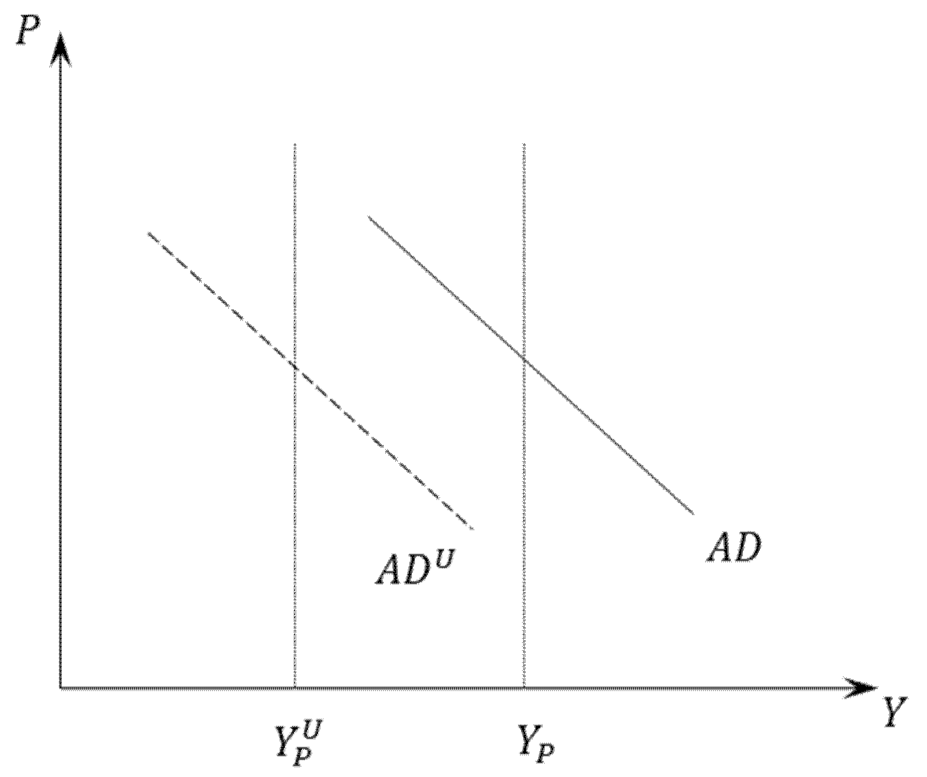
Concisely, tax evasion leads to a waste of economic resources. It follows that the A D   with tax evasion—which we call A D U —shifts to the left in the “price-output” space with respect to the “standard” A D (see Figure 1), namely, for a given price index ( P = P 0 ), the larger the share of tax evasion ( E ) and hidden economic activities ( φ ), the lower the aggregate expenditure of an economy.6

3. The Underground Economy and the Potential Output

The general finding of growth theory is that economic growth requires improvements in social infrastructures and the government’s fiscal policy is a key component of social infrastructures (Hall and Jones 1999; Romer 2006). Thus, an economic system with a larger share of tax evasion and hidden economic activities is merely a society with poor social infrastructures. Therefore, the potential output of an economy without (or with a lower share of) tax evasion and hidden economic activities ( Y p ) should be higher than the potential output of an economy with a larger share of tax evasion and hidden economic activities ( Y p U ), viz.:7
Y p > Y p U
In general, the underground sector is larger in the poorest economies (La Porta and Shleifer 2008), since the underground sector of the economy employs mostly unskilled labour and adopts backward technology (see, e.g., Albrecht et al. 2009). Therefore, a negative relationship between economic growth and the underground economy should exist (at least in the long run).8 Concisely, the official economy, which employs skilled labour and adopts more sophisticated technologies, is the engine of economic development (see, e.g., La Porta and Shleifer 2008).
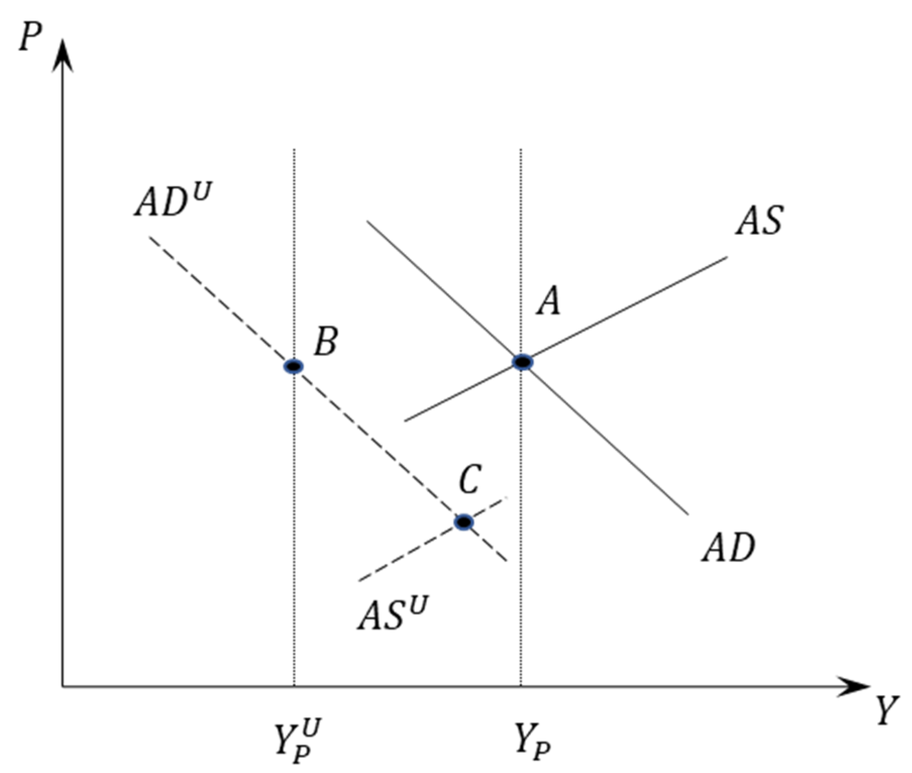
The AD-AS model with the underground economy, in the long run, is shown in Figure 2. The long-run effect of the underground economy on prices is, instead, an empirical question since it depends on both the reduction in aggregate expenditure and the reduction in potential output (see again Figure 2).

4. The AS with Undeclared Work

However, the presence in countries around the world and the persistence over time of the underground economy should involve the existence of (potential) positive effects on output, at least in the short run. Indeed, unemployment may be absorbed by undeclared work (see, e.g., Boeri and Garibaldi 2002, 2005; La Porta and Shleifer 2008; ILO 2011), thereby producing a (potential) positive effect on the actual level of output.
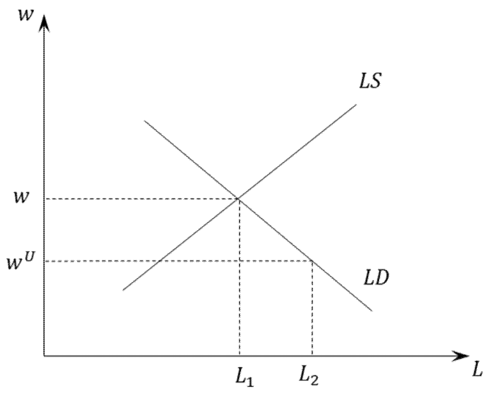
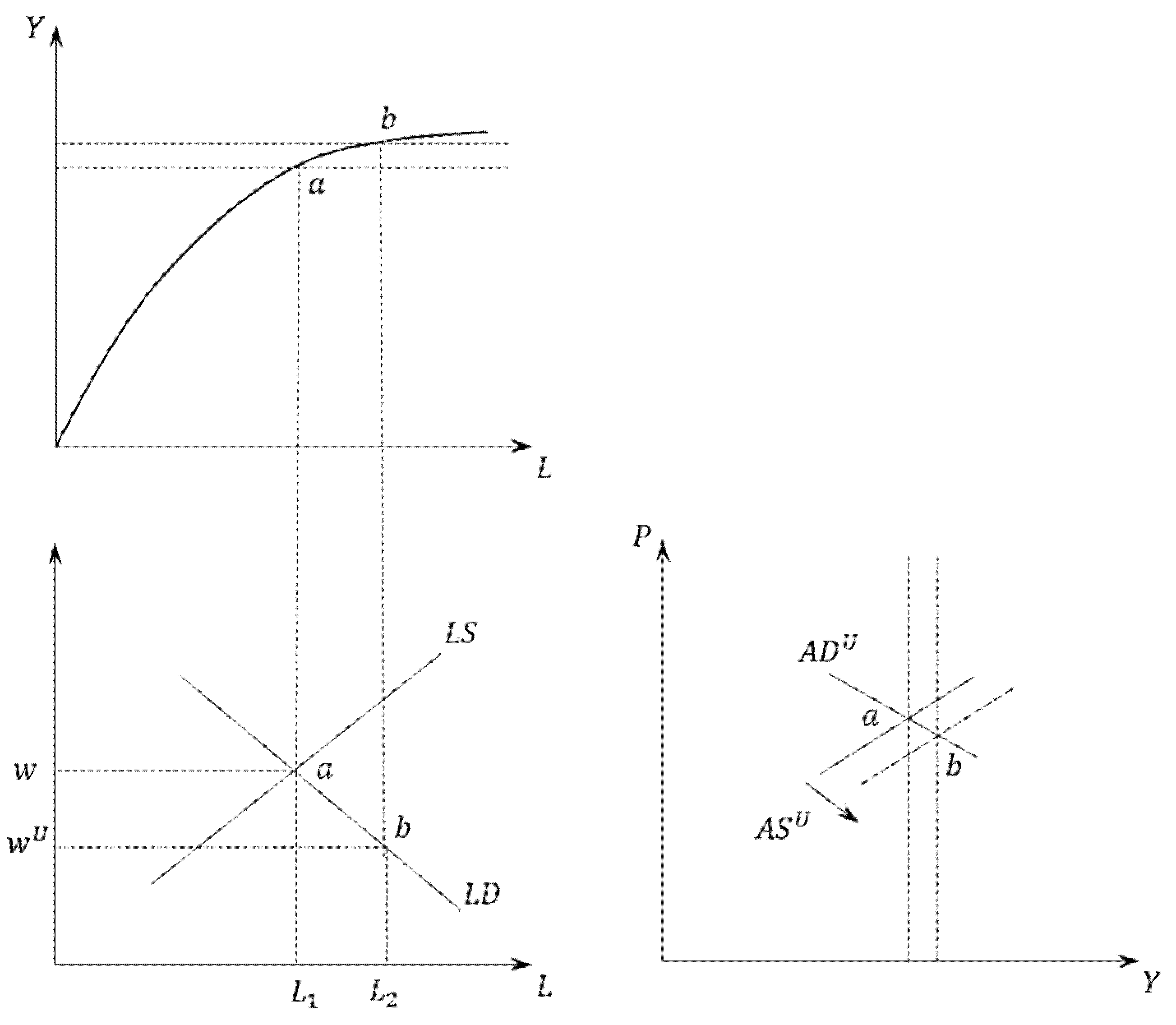
Actually, also registered (official) firms can make use of undeclared work for paying lower wages (the undeclared work is often unskilled labour). Concisely, w U < w , where w is the wage in the official sector and w U is the wage in the underground economy. Of course, unemployed workers agree to enter into a working agreement without an official contract, since w U > 0 , where 0 is the (zero) wage in the case of unemployment. Hence, in the labour market, there will be an increase in labour demand (employment) from L 1 to L 2 (see Figure 3), where ( L 2 L 1 ) denotes the workers in the underground economy. Assuming that the employment level L 1 is associated with the potential output, a kind of supply-side short-run positive shock occurs. This is straightforward to show. The AS is usually represented by a short-run production function (where the capital factor is fixed),
Y = f ( L )
with d Y d L > 0 and d 2 Y d L 2 < 0 . It links the labour market with the supply side of the goods market. The reduction in wages increases employment and output (in Figure 4 from point a to point b).
The aggregate supply moves downward in an economy with a large share of the underground sector (namely, the A S U moves downward) since the positive shock is due to a reduction in the undeclared labour cost. Indeed, this positive effect will be small or insignificant in an economy with a low share of both shadow economy and unemployment.9
The supply-side positive shock triggered by the underground economy is, by definition, temporary since there are no changes in the factors influencing the potential level of output (human capital and technological progress, for example). Instead, the decrease in unemployment—absorbed by the underground economy—will push up wages (in both sectors), thus decreasing overall employment. In the long run, therefore, the GDP will be equal to its potential value (once again).
However, in the presence of high unemployment, the supply-side positive shock could recur over time, thereby explaining the persistence of the underground economy, as well as its presence.

5. The Extended AD-AS Model: A Simple Comparison

This section focuses on the comparison between two economies that only differ with respect to the share of the underground economy, since the comparative statics (the effect of changes in exogenous variables on the equilibrium) of this extended AD-AS model does not change with respect to the “standard” AD-AS model. For example, an expansionary (recessionary) economic policy always shifts aggregate demand to the right (left).
For the sake of comparison, we assume that there are no (other) economic shocks; as a result, in an economy where the supply-side positive shock does not occur (because the share of the underground economy is small), the long-run equilibrium coincides with the short-run equilibrium.
As shown in Figure 5, the model features three kinds of “equilibrium”. Precisely:
  • Point C characterises the short-run equilibrium of an economy with a large share of the underground economy (where a supply-side positive shock exists);
  • Point B characterises the long-run equilibrium of an economy with a large share of the underground economy (where the potential output is lower);
  • Point A characterises the equilibrium of an economy with a low share of the underground economy (where both the potential output and the AD are higher). In this case, point A is both the short-run equilibrium and the long-run equilibrium.
It follows that the three equilibria of the model predict both different economic outcomes and alternative policy implications. We deepen this issue in the next sub-section.

Discussion: Economic Outcomes and Policy Implications

The previous results show that the developed theoretical model is able to derive both “positive statements” (what are the key economic results of the extended AD-AS model?) and “normative statements” (what should policymakers do?). Precisely, regarding the “positive statements”, this extended version of the AD-AS model states that:
  • In the short run, if the positive effect of the underground economy on both the employment level and the actual level of output is significant (i.e., the A S U lowers much) point C could be a potentially better situation than point A , since the cost of living is lower, and the purchasing power is higher. Furthermore, point C approaches point A in terms of output Y .
  • In the long run, instead, the reverse is true: point A is a better situation than point B , since the potential output is lower in the presence of a larger share of the underground economy.
Instead, regarding the “normative statements” and, thus, the policy implications, the model states that:
  • If the main goal of policy makers is the economic growth, they should devote their greatest efforts to fighting against the underground economy.
  • If the policymakers look especially at the present, the underground economy could be to some extent tolerated (in some countries, it seems that this happens).
It follows that an intertemporal socio-economic dilemma emerges for policymakers. Of course, the “normative” recommendations are more subjective and are inevitably based on the policymaker’s values.

6. Empirical Analysis

This section aims to carry out a simple empirical test of the main finding of the theoretical model: namely, the underground economy negatively affects economic growth, but in spite of this, it could have positive short-term effects on unemployment.
Thus, we perform a regional panel analysis in Italy. As mentioned above, Italy represents a remarkably interesting case study (a developed country where both shadow economy and unemployment are large).
We use the “one-way fixed effects” that capture the unobservable heterogeneity that is specific to each cross-section (regional) unit. The (balanced) panel used in this empirical analysis is composed of three main variables (regional GDP growth rate, regional share of shadow economy and regional unemployment rate) obtained for the 20 Italian regions (cross-section units) over 11 time periods (from 2005 to 2015), for a total of 220 observations. We collected the data from two main Italian sources: the Bank of Italy and ISTAT (The Italian National Institute of Statistics).10
In this empirical analysis, distributed lag (DL) models are used, since it takes time before an economic shock produces results:
Y i , t = a i + j = 0 n β j · X i , t j + ε i , t
where i = 1 20 denotes regions and a i are region-specific unobserved effects. In the distributed lag model (9) the reaction to Y i , t after a change in X i , t is distributed over a number of time periods ( t ). Precisely, it takes n + 1 time periods for the full effect of a change in X i , t to influence Y i , t (in the model, in fact, we have the current value of X i , t and n lagged terms). DL models can be estimated by simple OLS.
In order to save degrees of freedom, we apply a within transformation (which removes from the model any variable constant over time) and use five lags of the explanatory variable ( n = 4 ); thus, the model is the following:11
Y i , t = β 0 · X i , t + β 1 · X i , t 1 + β 2 · X i , t 2 + + β 3 · X i , t 3 + β 4 · X i , t 4 + ε i , t
The coefficients β j show the effects of X i , t on Y i , t . Precisely:
-
The coefficient β 0 is the impact in the current time period (it is usually called the impact multiplier);
-
The coefficients β 1 , β 2 , β 3 and β 4 are the effects in the previous time periods (they are usually called the interim multipliers);
-
The total effect of X i , t on Y i , t is instead called the long-run equilibrium effect and is given by: j = 0 4 β j = β 0 + β 1 + β 2 + β 3 + β 4 . Since in the long run long-run equilibrium (in a steady-state equilibrium, exactly): X i * = X i , t = X i , t 1 = X i , t 2 = X i , t 3 = X i , t 4 .
and, therefore, the model (10) in the long-run becomes:
Y i , t = X i * · j = 0 4 β j + ε i , t
In this empirical analysis, we estimate two DL models:
G D P i , t = j = 0 4 β j · S E i , t j + ε i , t
U N i , t = j = 0 4 β j · S E i , t j + ε i , t
where G D P i , t is the regional Gross Domestic Product growth rate; U N i , t is the regional unemployment rate, and S E i , t is the share of the regional shadow economy. We know that among these three key variables there is a potential reverse causality (an endogeneity problem). Hence, we merely interpret the regression coefficients as partial correlations.
The two main results of this empirical analysis are the following (see Table 1 for details):12
  • In model (12), the correlation between S E i , t and G D P i , t is always negative and, in many cases, statistically significant. Hence, both the short-run correlation and the long-run correlation between the shadow economy and economic growth are negative.
  • In model (13), instead, the correlation between S E i , t and U N i , t is negative (although quite small) and statistically significant only at the current time period (at the time t ). Hence, the short-run correlation between the shadow economy and unemployment is negative and, thus, the short-run correlation between the shadow economy and employment is positive.
Eventually, therefore, partial correlations seem to provide a first and preliminary confirmation of the main predictions of the theoretical model. A supply-side short-run positive shock triggered by the underground economy would seem to come true. By reducing unemployment, therefore, the underground economy could have a short-run positive effect on employment. However, the model confirms that the underground sector of the economy definitely damages economic growth (the output in the long-run).

7. Conclusions

While the factors determining the economic growth (such as technological progress and human capital), indirectly appear in the AD-AS model in determining the potential output, another important economic phenomenon, namely the underground economy, finds no place in the most popular and most studied macroeconomic model. This is an important gap to fill since the underground economy is a widespread phenomenon in both developed and developing countries. Furthermore, the underground economy can affect output (and, thus, employment) in both the short run and the long run. Hence, this phenomenon deserves to be included in the basic model for macroeconomic analysis.
By introducing—for the first time, to the best of our knowledge—the underground sector of the economy into the popular AD-AS model, the present paper aims at increasing the descriptive power of the model, without making it more complex. Indeed, this simple extension of the AD-AS model can explain both the presence (in countries around the world) and the persistence (over time) of the underground sector, despite its negative effects on both aggregate demand and economic growth. This is because, at least in the short run, the underground sector could increase the actual level of output by absorbing unemployment. Precisely, this well-known explanation in the related literature is formalised in this extension of the AD-AS model as a ‘supply-side short-run positive shock’. Concisely, the supply-side positive shock—i.e., an increase in both output and employment in the short-run—can explain the presence of the underground economy, while the possibility that this effect could recur over time (in the presence of high unemployment) could explain the persistence of the phenomenon.
Concisely, the present paper provides several non-trivial results. From a pedagogical standpoint, the paper includes an important economic phenomenon in the basic framework for macroeconomic analysis, thus increasing the descriptive power of the AD-AS model. From a theoretical standpoint, the model differentiates between positive statements and normative statements. Regarding the positive statements, the model states that the underground economy could have a short-run positive effect on employment, but in the long-run it hampers economic growth. Regarding the normative statements, the model shows that an intertemporal socio-economic dilemma exists for policymakers. Precisely, if the policymakers are “forward-looking”, the underground economy cannot be tolerated; whereas, if the policymakers are “near-sighted”, fighting against the underground economy is not a priority (namely, it can be tolerated). From an empirical point of view, a simple regional panel analysis in Italy seems to support the main predictions of this extended AD-AS model. Indeed, the correlation (in both short-run and long-run) between shadow economy and economic growth is negative; whereas, the short-run correlation between shadow economy and unemployment is negative (namely, the short-run correlation between shadow economy and employment is positive).
Eventually, which one of the two policies should be undertaken (“to tolerate or not to tolerate” the underground economy) depends on both values and goals of policymakers.

Funding

This research received no external funding.

Institutional Review Board Statement

Not applicable.

Informed Consent Statement

Not applicable.

Data Availability Statement

Data available upon request from the author.

Acknowledgments

The author wishes to thank the two anonymous referees for their many helpful comments and suggestions which have significantly improved the paper. A previous version of this paper (without the empirical part and with a simpler economic framework) appeared, for teaching purpose, in the Journal for Economic Educators, 18(1), 2018.

Conflicts of Interest

The author declares no conflict of interest.

Notes

1
Recent estimates suggest that the informal economy comprises more than half of the global labor force (International Labor Organization 2020) and around one third of GDP worldwide (Medina and Schneider 2018).
2
For more details about the “standard” AD-AS model, see, e.g., Mankiw (2015).
3
Mazhar and Méon (2017), instead, assume that a government has two instruments to finance a given level of public spending: a flat tax on output and seigniorage. Hence, their result of a positive relation between shadow economy and inflation relies on the possibility that a government can control monetary policy, namely there is not an independent central bank.
4
We consider φ as (partly) exogenous to taxes, since there are numerous other determinants affecting the share of the underground economy. Indeed, the size of the underground economy has many causes, including not only tax burden, but also corruption, organised crime, government instability, low quality of political institutions and weak rule of law (see, e.g., Medina and Schneider 2017, 2018).
5
When the goods market is in equilibrium, the aggregate expenditure is equal to real output ( Y = A D ).
6
Recall that in the ( P Y ) space, the AD is downward sloping because of three well-known effects: wealth effect (the negative effect of prices on consumption), interest rate effect (the negative effect of prices on investment) and international effect (the negative effect of prices on net exports). For the international effect to occur, of course, it needs to assume that the exchange rate does not change.
7
By definition, a higher level of potential GDP implies a lower natural unemployment rate. This is consistent with the empirical finding that (at least in advanced countries) productivity growth is strongly negatively correlated with unemployment in the long run (see Pissarides and Vallanti 2007).
8
Formally, the potential output can be represented by a long-run production function where the main inputs (in addition to the labour factor) are physical capital, infrastructure and public capital, human capital, entrepreneurship and technological progress. Of course, the potential output is not affected by demand factors and, thus, the AD movements will only have effects on prices.
9
The aggregate supply is upward sloping in the (𝑃 − 𝑌) space, meaning that when aggregate demand changes, firms adjust both price and quantity (for example, when aggregate demand increases, firms increase both price and quantity). Note that in this case there is a potential active role for economic policy: government and central bank can increase (by means of expansive economic policies) the actual level of GDP at the cost of higher inflation (an increase in the percentage change in the price index).
10
The Italian National Institute of Statistics (ISTAT) measures the regional underground employment rate, namely the ratio between the regional underground employment and the regional total employment. We use this variable as a proxy for the regional shadow economy. This is consistent with the theoretical model where the underground economy plays a key role on the supply-side of the labour market.
11
Usually, the optimal lag-length is obtained by using a relatively large number of lags and choosing the model with the lowest value of AIC, SBC or any other criterion. However, this approach generates two considerable problems: (1) a large number of lags can give rise to a severe multicollinearity problem; (2) a large number of lags means a considerable loss of degrees of freedom, i.e., many additional parameters to estimate. Another solution, it could be the so-called “Koyck transformation” that introduces a lagged term of the dependent variable. In that case the DL model (9) becomes: Y i , t = a i · ( 1 λ ) + β 0 · X i , t + λ · Y i , t 1 + η i , t , where 0 < λ < 1 , β 0 is the immediate effect of X i , t on Y i , t , while β 0 1 λ is the long-run effect of X i , t on Y i , t under the steady-state equilibrium condition, i.e., Y i , t = Y i , t 1 . In dynamic panel models that include the presence of a lagged dependent variable among the regressors, however, the traditional OLS estimators are biased and, thus, different and more sophisticated methods of estimation need to be used.
12
Note that the null hypothesis that all region-specific unobserved effects are null (all a i = 0) is rejected. Thus, the fixed-effects model seems to be an appropriate specification.

References

  1. Abdel-Latif, Hany, Bazoumana Ouattara, and Phil Murphy. 2017. Catching the mirage: The shadow impact of financial crises. Quarterly Review of Economics and Finance 65: 61–70. [Google Scholar] [CrossRef] [Green Version]
  2. Aizenman, Joshua, Yothin Jinjarak, Hien Thi Kim Nguyen, and Donghyun Park. 2019. Fiscal space and government-spending and tax-rate cyclicality patterns: A cross-country comparison, 1960–2016. Journal of Macroeconomics 60: 229–52. [Google Scholar] [CrossRef]
  3. Albrecht, James, Lucas Navarro, and Susan Vroman. 2009. The effects of labour market policies in an economy with an informal sector. Economic Journal 119: 1105–29. [Google Scholar] [CrossRef]
  4. Asada, Toichiro, Pu Chen, Carl Chiarella, and Peter Flaschel. 2006. Keynesian dynamics and the wage-price spiral. A baseline disequilibrium approach. Journal of Macroeconomics 28: 90–130. [Google Scholar] [CrossRef] [Green Version]
  5. Bajada, Christopher. 2003. Business cycle properties of the legitimate and underground economy in Australia. Economic Record 79: 397–411. [Google Scholar] [CrossRef]
  6. Boeri, Tito, and Pietro Garibaldi. 2002. Shadow Activity and Unemployment in a Depressed Labour Market. CEPR Discussion Papers, 3433. June. Available online: https://papers.ssrn.com/sol3/papers.cfm?abstract_id=323388 (accessed on 17 August 2002).
  7. Boeri, Tito, and Pietro Garibaldi. 2005. Shadow sorting, NBER Chapters. In NBER International Seminar on Macroeconomics. Edited by Jeffrey A. Frankel and Christopher Pissarides. Cambridge: MIT Press, pp. 125–63. [Google Scholar]
  8. Catalina, Granda, and Danny García. 2020. Informality, Tax Policy and the Business Cycle: Exploring The Links. Documento de Trabajo, Alianza EFI-Colombia Científica, Número de serie: WP5-2020-001. Bogotá: Alianza EFI. [Google Scholar]
  9. Chen, Pu, and Peter Flaschel. 2005. Keynesian Dynamics and the Wage-Price Spiral: Identifying Downward Rigidities. Computational Economics 25: 115–42. [Google Scholar] [CrossRef]
  10. Chen, Pu, and Peter Flaschel. 2006. Measuring the interaction of Wage and Price Phillips Curves for the US economy. Studies in Nonlinear Dynamics and Econometrics 10: 10–35. [Google Scholar]
  11. Chen, Pu, Carl Chiarella, Peter Flaschel, and Willi Semmler. 2006. Keynesian macrodynamics and the Phillips curve. An estimated baseline macro-model for the U.S. economy. In Quantitative and Empirical Analysis of Nonlinear Dynamic Macromodels. Contributions to Economic Analysis. Edited by Carl Chiarella, Reiner Franke, Peter Flaschel and Willi Semmler. Amsterdam: Elsevier. [Google Scholar]
  12. Çiçek, Deniz, and Ceyhun Elgin. 2011. Cyclicality of fiscal policy and the shadow economy. Empirical Economics 41: 725–37. [Google Scholar] [CrossRef]
  13. Colombo, Emilio, Luisanna Onnis, and Patrizio Tirelli. 2016. Shadow economies at times of banking crises: Empirics and theory. Journal of Banking & Finance 62: 180–190. [Google Scholar]
  14. Colombo, Emilio, Lorenzo Menna, and Patrizio Tirelli. 2019. Informality and the labor market effects of financial crises. World Development 119: 1–22. [Google Scholar] [CrossRef]
  15. Dutt, Amitava Krishna, and Peter Skott. 2006. Keynesian Theory and the AD–AS Framework: A Reconsideration. Contributions to Economic Analysis 277: 149–72. [Google Scholar]
  16. Elgin, Ceyhun. 2012. Cyclicality of Shadow Economy. Economic Papers 31: 478–90. [Google Scholar] [CrossRef]
  17. Elgin, Ceyhun, and Ferda Erturk. 2019. Informal economies around the world: Measures, determinants and consequences. Eurasian Economic Review 9: 221–37. [Google Scholar] [CrossRef]
  18. Elgin, Ceyhun, and Burak R. Uras. 2013. Public debt, sovereign default risk and shadow economy. Journal of Financial Stability 9: 628–40. [Google Scholar] [CrossRef] [Green Version]
  19. Eng, Yoke-Kee, and Chin-Yoong Wong. 2008. A short note on business cycles of underground output: Are they asymmetric? Economics Bulletin 3: 1–10. [Google Scholar]
  20. Flaschel, Peter, Gangolf Groh, Christian Proaño, and Willi Semmler. 2008a. Estimation and Analysis of an Extended AD–AS Model. Topics in Applied Macrodynamic Theory, DMEF 10: 137–212. [Google Scholar]
  21. Flaschel, Peter, Reiner Franke, and Christian Proaño. 2008b. On the (In)Determinacy of New Keynesian Models with Staggered Wages and Prices. Mimeo: Bielefeld University. [Google Scholar]
  22. Frankel, Jeffrey, Carlos Vegh, and Guillermo Vuletin. 2013. On graduation from fiscal procyclicality. Journal of Development Economics 100: 32–47. [Google Scholar] [CrossRef] [Green Version]
  23. Hall, Robert E., and Charles I. Jones. 1999. Why do some countries produce so much more output per worker than others? Quarterly Journal of Economics 114: 83–116. [Google Scholar] [CrossRef]
  24. International Labour Organization (ILO). 2011. Statistical Update on Employment in the Informal Economy. Geneva: ILO. [Google Scholar]
  25. International Labor Organization. 2020. 13. Informal Economy. Available online: https://www.ilo.org/global/topics/dw4sd/themes/informal-economy/lang--en/index.htm#33 (accessed on 8 October 2021).
  26. La Porta, Rafael, and Andrei Shleifer. 2008. The unofficial economy and economic development. Brookings Papers on Economic Activity 39: 275–363. [Google Scholar]
  27. Loayza, Norman, and Jamele Rigolini. 2011. Informal Employment: Safety Net or Growth Engine? World Development 39: 1503–15. [Google Scholar] [CrossRef]
  28. Mankiw, N. Gregory. 2015. Essentials of Economics, 7th ed. North Way: Cengage Learning EMEA. [Google Scholar]
  29. Mazhar, Ummad, and Pierre-Guillaume Méon. 2017. Taxing the unobservable: The impact of the shadow economy on inflation and taxation. World Development 90: 89–103. [Google Scholar] [CrossRef] [Green Version]
  30. Medina, Leandro, and Friedrich Schneider. 2017. Shadow Economies around the World: New Results for 158 Countries over 1991–2015. CESifo Working Papers, No. 6430. Munich: CESifo. [Google Scholar]
  31. Medina, Leandro, and Friedrich Schneider. 2018. Shadow Economies Around the World: What Did We Learn Over the Last 20 Years? International Monetary Fund (IMF) Working Paper No. 18/17. Washington, DC: IMF. [Google Scholar]
  32. Pissarides, Christopher, and Giovanna Vallanti. 2007. The impact of TFP growth on steady-state unemployment. International Economic Review 48: 607–40. [Google Scholar] [CrossRef]
  33. Romer, David. 2006. Advanced Macroeconomics, 3rd ed. New York and London: McGraw-Hill. [Google Scholar]
  34. Schneider, Friedrich, and Dominik H. Enste. 2000. Shadow economies: Size, causes, and consequences. Journal of Economic Literature 38: 77–114. [Google Scholar] [CrossRef] [Green Version]
  35. Schneider, Friedrich, and Dominik H. Enste. 2002. Hiding in the Shadows. The Growth of the Underground Economy. Economic Issues N° 30, International Monetary Fund (March). Washington, DC: IMF. [Google Scholar]
  36. Toichiro, Asada, Pu Chen, Carl Chiarella, and Peter Flaschel. 2006. AD–AS and the Phillips Curve: A Baseline Disequilibrium Model. Contributions to Economic Analysis 277: 173–227. [Google Scholar]
  37. Toichiro, Asada, Carl Chiarella, Peter Flaschel, and Proaño Christian. 2007. Keynesian AD-AS, Quo Vadis? Working Paper Series 151; Sydney: Finance Discipline Group, UTS Business School, University of Technology. [Google Scholar]
  38. Torgler, Benno. 2007. Tax Compliance and Tax Morale: A Theoretical and Empirical Analysis. Cheltenham and Northampton: Edward Elgar Publishing. [Google Scholar]
  39. Vegh, Carlos, and Guillermo Vuletin. 2015. How Is Tax Policy Conducted over the Business Cycle? American Economic Journal: Economic Policy 7: 327–70. [Google Scholar] [CrossRef] [Green Version]
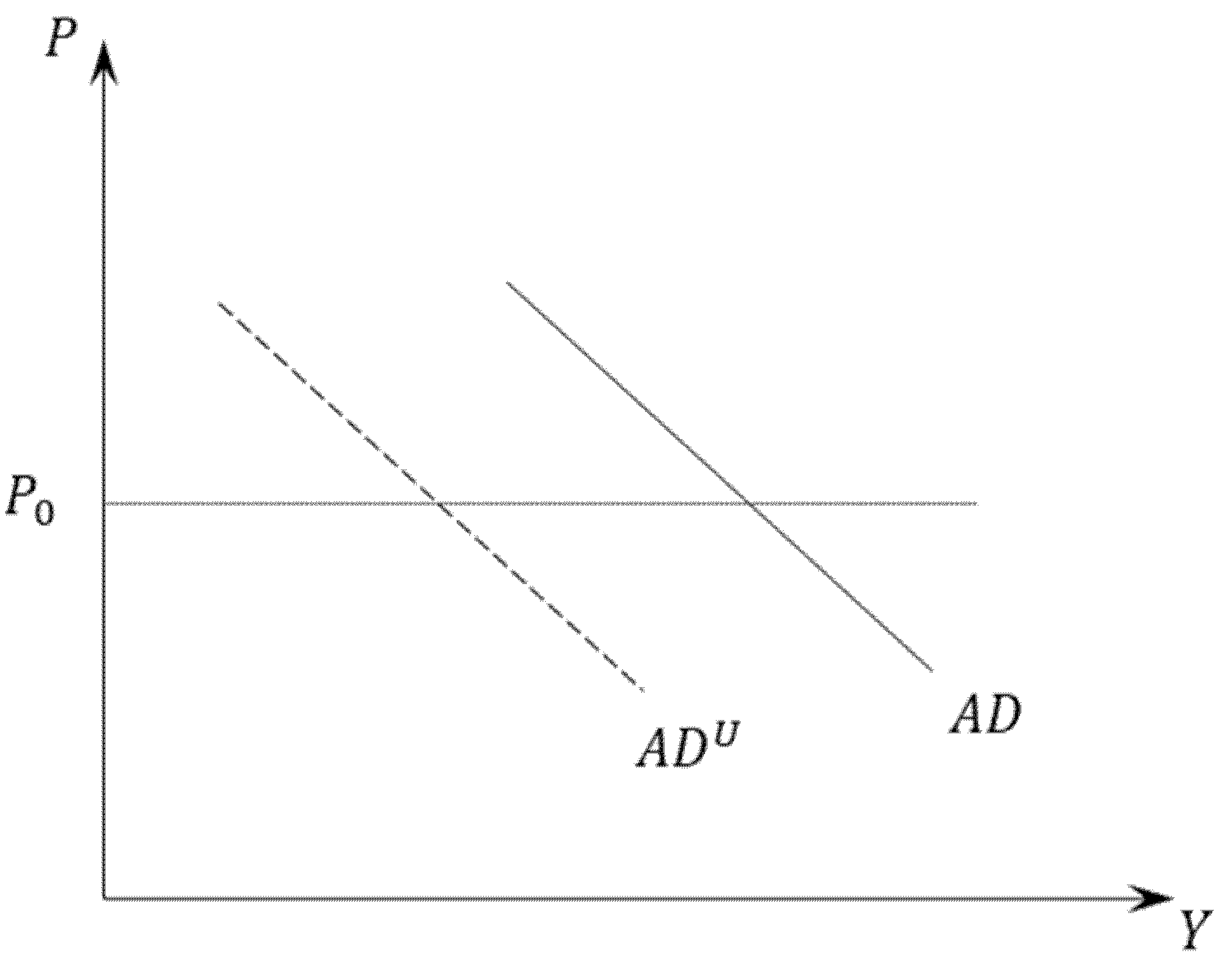
Figure 1. The AD with hidden economic activities and tax evasion.
Economies 09 00170 g001
Figure 2. The AD-AS model with the underground economy in the long run.
Economies 09 00170 g002
Figure 3. Unemployed workers and undeclared work.
Economies 09 00170 g003
Figure 4. Undeclared work and supply-side positive shock: from labour market to goods market.
Economies 09 00170 g004
Figure 5. The AD-AS model with the underground economy: short- and long-run.
Economies 09 00170 g005
Table 1. The (short-run and long-run) impact of shadow economy on growth and unemployment in Italy.
VariableModel (12)
G D P i , t
Model (13)
U N i , t
S E i , t −0.241 (2.49) *−0.017 (2.01) *
S E i , t 1 −0.236 (2.19) *0.101 (1.65)
S E i , t 2 −0.258 (1.67)−0.012 (1.51)
S E i , t 3 −0.216 (1.71)0.099 (1.79)
S E i , t 4 −0.188 (2.08) *0.012 (1.84)
Statistical tests
F test
all a i = 0
Prob > F
0.000
Prob > F
0.000
R2 overall0.46350.5072
Observations
220
Note: t-statistic in parentheses. * denotes statistical significance at the 5% level (p-value < 0.05): t-statistic > 2.
Publisher’s Note: MDPI stays neutral with regard to jurisdictional claims in published maps and institutional affiliations.