1. Introduction
In recent years, certain abnormal behaviors (calendar effects) were revealed to have an effect on the return on financial assets, thereby increasing research in this area. One of the effects, which stands as evidence against the market efficiency hypothesis, is called the month-of-the-year effect.
Renowned academics have investigated this topic, concluding that it breaks down into three anomalies: (i) the “January effect”, which maintains that the average return on shares tends to be higher in January compared to the other months of the year; (ii) the “May-to-October effect”, or the “Halloween effect”, which indicates that the average return on shares during the summer and autumn is lower compared to the months that make up the two missing seasons (spring and winter); and, finally, (iii) the “October Effect”, which maintains that October is the month of the year with the lowest average shareholder returns.
Thus, considering the effects mentioned above, adequately disaggregated into each of its anomalies, this paper aims to ascertain its applicability/existence in the European, American, Australian, and Asian markets.
Our contribution to the literature comes from our analysis of the abnormal returns that may have resulted from these three month-of-the-year anomalies, allowing us to ascertain which anomalies, if any, had an impact on the capital market, and what the direction of that impact might have been, focusing upon the 1990–2013 period for European, American, Australian, and Asian markets. We have thus ascertained whether or not calendar anomalies offer opportunities for investors. This research intends to contribute to our understanding of whether these calendar anomalies occur in the stock markets in a persistent and regular way, and therefore whether they are fruitful strategies for investors. Our main findings point to a significant Halloween effect, as expected, and significant unexpected January and October effects, mainly in the post-dotcom-bubble period, for globally diversified portfolio investment strategies. In global terms, average returns in winter and spring could be 1.2% higher compared to average returns in summer and autumn, while in months other than October, average returns could be 1% lower compared to the average returns in October, and average returns in January could be 1.6% lower compared to the average returns of the remaining months. Only in the pre-dotcom-bubble period do average returns in January seem to perform 1.4% higher than the remaining months for globally diversified portfolio investment. The Halloween effect appears to be a fruitful strategy for the FTSE, DAX, Dow Jones, BOVESPA, and N225 indexes taken one-by-one, proving to be an ongoing investment strategy for those indexes.
Compared to the literature, our research focuses on a wide geographical range of capital markets and promotes a global and comparable view upon the topic.
In the following sections, a literature review is performed, followed an outline of the methodology selected, our results analysis, and finally our main conclusions.
2. Literature Review
The leading explanations for calendar effects are associated with several factors, such as trends in investor behavior, institutional prerequisites, and the publication of negative information. Of the range of calendar anomalies pointed out in the literature, most significant might be the month-of-the-year effect (
Lean et al. 2007).
According to
Alrabadi and Al-Qudah (
2012), the month-of-the-year effect includes three anomalies: (i) the January effect; (ii) the May-to-October effect (also known as the Halloween effect); and (iii) the October effect. However, according to the January effect, the return on shares in January tends to be higher than the returns provided in the remaining months of the year. On the other hand, the Halloween effect refers to the fact that the returns on shares tend to be lower in the summer and autumn months compared to the spring and winter months. Finally, the October effect is based on the premise that the returns shown in October are lower than the rest of the year.
The first academic reference to the seasonality in question is by
Wachtel (
1942). However, the first empirical evidence associated with the January effect saw daylight only 30 years after. The researchers responsible for this empirical finding,
Rozeff and Kinney (
1976), note that, between 1904 and 1974, New York Stock Exchange (NYSE) shares obtained an average return of 3.48% in January, in contrast to average monthly returns of 0.42% in each of the remaining months of the year. It should be noted that the effect is often referred to as an effect intrinsic to the reality of small businesses (
Rozeff and Kinney 1976;
Reinganum 1983).
Nevertheless, the January effect is also documented in countries other than the US (
Gultekin and Gultekin 1983), and in other securities, such as bonds (
Fama and French 1993). It should be noted that studies focus on the ability of investors to take advantage of the January effect through the use of mutual investment funds and future market indexes (
Booth and Keim 2000;
Hensel et al. 2000;
Rendon and Ziemba 2005).
Keim (
1983) also presents a fascinating study showing that more than half of the market premium was obtained in the first days of January during the years 1963 to 1979.
Other authors, such as
Roll (
1983) and
Reinganum (
1983), validate the January effect’s existence, saying that it is more significant in small companies. To this finding,
Branch and Chang (
1990) add that the effect proves to be more significant in small companies with low-priced shares, and, in turn,
DeBondt and Thaler (
1985,
1987) state that the significance of the effect is higher in small companies that, in comparison to others, have underperformed in the past. Regarding the various explanations for the January effect, the literature gives some prominence to two hypotheses: the tax-loss selling hypothesis (
Wachtel 1942) and the window dressing hypothesis (
Lakonishok and Smidt 1988).
The tax-loss selling hypothesis suggests that investors sell the “losing” shares in their portfolio at the end of the year to gain a tax benefit, and are only able to reinvest the paid-up capital in January (
Reinganum 1983). The window dressing hypothesis states, in turn, that investors sell certain stocks at the end of the year to present a more acceptable stock portfolio to equity holders in year-end reports, creating such abnormal returns in January.
In addition to the two abovementioned explanatory hypotheses, some researchers have identified market microstructure effects, such as bid–ask spread (
Stoll and Whaley 1983) and thin trading, as essential factors explaining abnormal returns in January (
Roll 1981 and Roll 1983).
Kohers and Kohli (
1992) link the anomaly to the business cycle, and
Aguiar et al. (
1997) argue that the high returns in January are related to a large volume of commercial transactions associated with lower real interest rates. End-of-year events are pointed to by other authors as possible explanations. It should be noted, at this point, that
Ogden (
1990) associates the January effect with cash transactions verified at the end of the year or with liquidity. On the other hand, risk is pointed to as the most preponderant element for the explanation of the January phenomenon.
Rozeff and Kinney (
1976);
Tinic and West (
1984);
Rogalski and Tinic (
1986);
Gultekin and Gultekin (
1983);
Chang and Pinegar (
1986);
Kramer (
1994) and
Kim (
2006) argue that acceptance of the risk factor is a cause of the January effect.
Regarding the second anomaly that constitutes one of the month-of-the-year effects, specifically the Halloween effect,
Bouman and Jacobsen (
2002) say that this anomaly appears in the financial market and has solid potential as an opportunity for abnormal returns. Already referenced in the
Financial Times in May 1964, according to studies by
Jacobsen and Zhang (
2010);
Levis (
1985);
Hirsch (
1986) and
Bouman and Jacobsen (
2002), the so-called Halloween effect follows the “sell in May and go away” strategy, inherent to which is the assumption that returns on securities from May to October tend to be lower than those evidenced in the remaining months of the year. In this context, it should be noted that this assumption is reasoned by the fact that wealthy investors enjoy holidays during this period, leaving aside, for a certain period, their investments in the financial market.
From an analysis of the monthly return on shares in 37 different countries in the period between January 1970 and August 1998,
Bouman and Jacobsen (
2002) found, in their widely recognized study, that in 36 of them, the average monthly returns were lower between May and October compared to the other months of the year. This assessment had a statistical significance of 1% in 10 countries and 10% in another 20 countries.
Bouman and Jacobsen (
2002) also show that, in some countries, the presence of the Halloween effect is much more lasting. For example, in the United Kingdom, from the longest series of data analyzed (300 years), and at a significance level of 10%, the effect has been observed since 1694. In turn, at a level of significance of 5%, the presence of the effect has been demonstrated in the Japanese and Canadian markets for 1920 and 1933 onwards, respectively, while its existence in the German market has been verified for 1950 and after.
Several authors provide evidence for the absence of the Halloween effect. We highlight here research by
Lucey and Zhao (
2008). They, through an examination of the Halloween effect in the United States stock market between 1926 and 2002, conclude that, in the long term, the evidence of the effect is thin and, when observable, it seems to be due to the January effect. They further observe that the Halloween strategy does not surpass the “Buy and Hold” strategy.
Bouman and Jacobsen (
2002) analyzed the impact of the role of risk, the correlation between markets, the January effect, the increases in interest rates, the changes in the amount transacted, the association with a given activity sector, and the existence of a seasonal factor influencing the supply of market information on the Halloween effect within the scope of market securities returns. However, the researchers conclude that none of these aspects appears to provide a plausible explanation for the effect. However,
Kamstra et al. (
2003) claim that the existence of the Halloween effect is due to the impact of seasonal affective disorder (SAD) on share returns. In detail, SAD refers to the inverse relationship that some researchers believe exists between the decrease in daily hours during the fall and investors’ depression index. In this context,
Maberly and Pierce (
2004) say that the documentation compiled by
Bouman and Jacobsen (
2002), which supposedly reveals a significant Halloween effect in the United States market, seems to be caused by the presence of two outliers, and therefore does not reveal the existence of a Halloween effect. On the other hand,
Cao and Wei (
2005) associate share returns with changes in air temperature during the year, based on psychological studies that support the impact of extreme air temperatures (very high or very low) on human behavior.
Otherwise known as the Mark Twain effect, the October effect is synonymous with a theory that holds that the average return on shares during October is significantly lower than that achieved in the remaining months of the year (
Cadsby 1989). In his classic book,
Twain (
1981) says “October. This is one of the peculiarly dangerous months to speculate stocks in”. Apologists for the October effect claim that it is directly related to severe adverse events in the stock markets in the middle of October. In line with their beliefs, there are some investors and professionals in the financial ecosystem who put aside specific savings to cover the harmful consequences on their share portfolios during that month. However, some also argue that the October effect is more of a superstition than a well-documented phenomenon. For those seeking to validate the phenomenon, the theory is often presented with examples of catastrophic events that had damaging effects on the stock market in the middle of October. The Great Depression of the 1930s, caused by the breakdown of financial markets in year 1929 is often cited. Further, the sudden crash of 1987 occurred in October, also supposedly demonstrating the October effect.
Indeed, from 1929 and during October, the days of negotiations that are known as “Black Monday”, “Black Tuesday”, and “Black Thursday” took place. During these dark days, the Dow Jones Industrial Average index (New York) registered steep drops of 12% (9 October 1929 (Black Tuesday)), 11% (24 October 1929 (Black Thursday)), and, later, 23% (19 October 1987 (Black Monday)). From another perspective, it can be seen that, since 1928, 37 drops have occurred in October. Across these 37 times, shares were sold, losing –14.3% in value on average. Even if the S&P 500 index has shown no October effect after 1993, according to
Szakmary and Kiefer (
2004), prior to 1993, the same conclusion is not valid.
The stochastic dominance (SD) approach, as a technique used to select the best investment alternatives through the mathematical comparison of the respective accumulated distribution functions, is used in parallel with the linear regression model. It is applied when one intends to examine seasonality, both in stock and bond markets, as exemplified by the studies by
Seyhun (
1993) and
Wingender and Groff (
1989) to assess the January and day-of-the-week effects, respectively, for the US stock market. Additionally, the study by
Lean et al. (
2007) applies the SD model, referring to its advantages over parametric tests. Note that it makes no assumptions about the nature of the distribution, unlike traditional parametric tests relying on mean and variance, thus omitting important information from relevant moments.
Despite the advantages of SD, this approach was not used in this research because of difficulties with its implementation, requiring numerical optimization in certain cases. For example,
Meyer’s (
1977) SD application required the solution of a control optimization problem. Moreover, the convex SD rules for simultaneous comparison of two or more perspectives require optimization (
Fishburn 1974). Our approach for this research ensures the advantage of the linear regression function with the inclusion of dummy variables in the calculation of calendar effects, as identified by
Bouman and Jacobsen (
2002).
3. Methodology and Data
This paper examines the following research hypotheses, based on the literature review above, testing for:
- (i)
The “January effect”, where average stock returns in January tend to be higher compared to the other months of the year;
- (ii)
The “Halloween effect”, where average stock returns in summer and autumn tend to be lower compared to the spring and winter months; and
- (iii)
The “October effect”, where average stock returns in October tend to be the lowest of the year.
The research methodology follows three steps. First, we compute monthly instantaneous returns from daily data. Second, we analyze monthly returns in order to verify data stationarity and identify differences between monthly returns, considering the months covered by each month-of-year effect. Third, we analyze each month-of-the-year effect’s statistical significance, in order to verify whether those effects offer consistent opportunities for investors.
The data collected cover a maximum of 24 years (1990–2013), depending on the index used. The data are split into two periods: before and after the dotcom bubble. The cut-off in this research is 30 September 2001, when most of the losses inflicted by the explosion of the dotcom bubble had been felt. The significance of the month-of-the-year effects is therefore analyzed over the following periods:
From January 1990 to December 2013—288 months over the total period;
From January 1990 to September 2001—141 months over the pre-dotcom-bubble period; and
From October 2001 to December 2013—147 months over the post-dotcom-bubble period.
It is important to note that the different indexes used in this research were modeled in order to obtain monthly logarithmic returns, as expressed in the following Equation (1):
where
corresponds to the closing price of an index on the last day of the month and
is equivalent to the closing price of the same index on the last day of the month prior to
.
Once the monthly logarithmic returns (1) were obtained, traditional OLS linear regression was applied using dummy variables to ascertain the existence of the three anomalies that comprise the month-of-the-year effects at a statistical level.
Following
Bouman and Jacobsen (
2002), for the January effect, the linear regression equation takes the following specification:
Dependent variable represents the index’s instantaneous monthly returns. Single dummy independent variable assumes 1 for January returns and 0 for each of the remaining months. Average excess returns for January are given by the coefficient, average returns for remaining months are given by , and is the error term. Average monthly returns for January are given by .
Regarding the Halloween effect, the following equation is used:
Dependent variable represents the index’s instantaneous monthly returns. Single dummy independent variable assumes 1 for each of the months between November and April (these months included) and 0 for each of the remaining months. Average returns for the months between May and October are given by the intercept, average excess return for the months between November and April are given by the coefficient, and is the error term. Average monthly returns between November and April are given by .
For the October effect, a similar equation to Equation (2) is used:
Dependent variable represents the index’s instantaneous monthly returns. Single dummy independent variable assumes 0 for October returns and 1 for each of the remaining months. Average returns for October are given by the intercept, average excess returns for remaining the months are given by the coefficient and is the error term. Average monthly returns for months which are not October are given by .
The four continent indexes data came from the Finance Yahoo website for: (i) PSI20 (Portuguese Stock Index): Portugal/Europa; (ii) FTSE (Financial Times Stock Exchange): London/Europe; (iii) DAX (Deutscher Aktien Index): Germany/Europe; (iv) DJIA (Dow Jones Industrial Average): USA/America; (v) NASDAQ (National Association of Securities Dealers Automated Quotations): North America/America; (vi) BOVESPA (São Paulo Stock Exchange): Brazil/America; (vii) HSI (Hang Seng Index): China/Asia; (viii) N225 (Nikkei Stock Average): Japan/Asia; and (ix) NZ50 (New Zealand Stock Exchange): Australia/Oceania.
These nine indexes were chosen according to their relevance in the world stock market and also in order to make it possible to verify whether the anomalies occur at a global level, continental level, and/or at a stock market level.
SPSS software was used to analyze the outputs.
4. Results
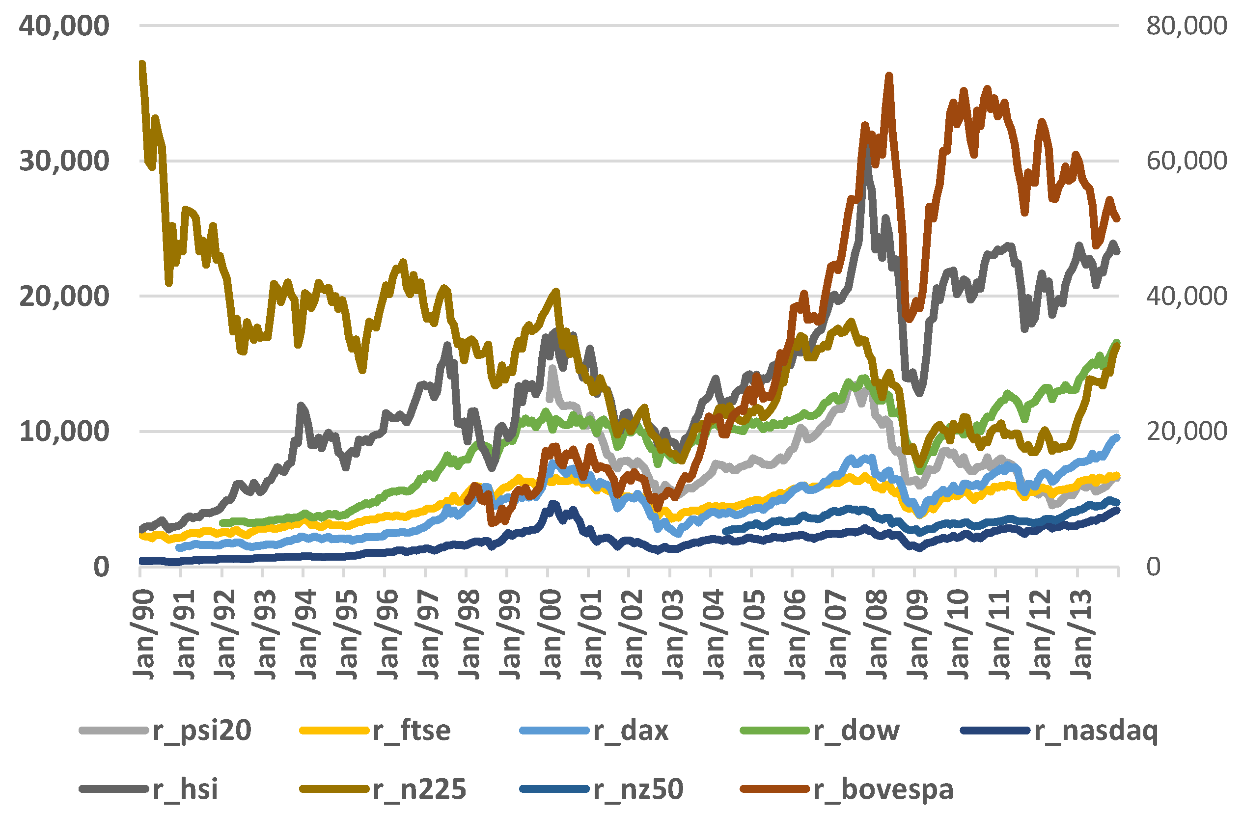
Figure 1 shows the evolution of all the indexes from 1990 to 2013. All show a growth trend, except the N225. BOVESPA, the only index using the second Y-axis scale, had by far the most positive performance. Note that all index data clearly show the dotcom bubble ending late 2001 and the financial subprime crisis in late 2008.
Figure 2 below shows all nine indexes’ monthly returns, where data stationarity can be observed. Moreover, for each index, a monthly return Dickey–Fuller test for unit root was performed without evidence of autocorrelation.
Prior to the OLS linear regression analysis, in order to become acquainted with the returns differences (positive or negative) for each of the three month-of-the-year anomalies and their accordance with the existing literature, average monthly returns differences for the months covered by each month-of-the-year effect were computed, with the results shown in
Table 1,
Table 2 and
Table 3.
Annual data are split into two periods only for the average monthly returns difference analysis. For the January effect, average instantaneous monthly returns for January were compared with average instantaneous monthly returns from the remaining 11 months, as if they were a single month. For the Halloween effect, average instantaneous monthly returns from November to April were compared with average instantaneous monthly returns from May to October, as if they were two single months. Finally, for the October effect, average instantaneous monthly returns for October were compared with average instantaneous monthly returns from the remaining 11 months, as if they were a single month.
The January average monthly returns difference can be seen in
Table 1.
Table A1,
Table A2 and
Table A3 contain output details, including results of the tests for statistical significance.
For the pre-dotcom-bubble period, the January effect appears to be active globally, with extra 2.38% average monthly return in January. Moreover, January is the month with the highest average return. In the post-dotcom-bubble period, January shows a 1.01% lower average return compared to the remaining months. Statistical significance for these findings can be found in
Table A1,
Table A2 and
Table A3. In addition, January shows a negative average monthly excess return in all one-by-one indexes for the post-dotcom-bubble period, with only the FTSE being statistically significant.
For the January effect total period results, primarily influenced by the post-dotcom-bubble period, not a single index shows a statistically significant January effect, nor is it evident globally.
Regarding the Halloween effect total period, which is significantly influenced by the pre-dotcom-bubble period results, the output shows statistical significance for excess average monthly returns in most of the indexes individually and for all of them globally, even with a dubious January effect. Pre- and post-dotcom-bubble periods are no exception globally, with statistical significance for November to April average monthly excess returns compared to the remaining months (
Table 2,
Table A1,
Table A2 and
Table A3). Individually, DAX, Dow Jones, and BOVESPA seem to have higher average returns in winter and spring in the pre-dotcom-bubble period. Only N225 individually shows a consistent average monthly excess return in winter and spring in the post-dotcom-bubble period.
From a global point of view or for all indexes one-by-one, all have shown higher average monthly returns for winter/spring, in all three periods, except the HSI in the post-dotcom period.
A curious finding that comes from the analysis of the Halloween effect is within the pre-dotcom-bubble period, which, on average, reveals an average monthly return for winter compared to summer that is 1.5 times higher than the same average monthly return difference in the post-dotcom-bubble period.
In this context, it should be also noted that winter/spring higher average monthly returns decrease considerably between the pre-dotcom-bubble and the post-dotcom-bubble periods for Europe and North America. It is not entirely unfounded to admit that there is a fading Halloween effect in these continents, with Asia showing the opposite trend over time.
As for the October effect, and according to the results (see
Table 3,
Table A1,
Table A2 and
Table A3), it seems that October average returns become higher compared to the remaining months, instead of being lower, as expected. Only the PSI20 and NASDAQ in the pre-dotcom-bubble period, the N225 and NZ50 in the total and post-dotcom-bubble periods have shown lower average monthly returns in October, and neither are statistically significant. The PSI20 and NASDAQ had lower average returns in October in the former period, which became higher average returns in the latter period. The N225 had higher average returns in October in the former period, which became lower average returns in the latter period. Neither are statistically significant, as shown in
Table A1,
Table A2 and
Table A3.
Indeed, for the global analysis, total and post-dotcom-bubble periods reveal a statistically significant average monthly (positive) excess return in October, which does not corroborate the literature.
In addition to monthly returns difference analysis, we verify whether return and risk are positively related, in line with the essence of the financial principle that maintains that higher returns are the fair compensation for the higher levels of risk assumed. For the January, Halloween, and October effects, no relationship was found between the two (risk/return) variables. In fact, for our data sample, it can be seen in general that effects with higher returns reveal lower variance.
According to
Table 4, the January effect analysis reveals that there are no statistically significant differences between the indexes’ average monthly returns in January and non-January months for any of the three periods, taking the indexes one-by-one. An exception is the FTSE in the post-dotcom-bubble period, which had a −2.3% average monthly excess return compared to the non-January months. Globally, there are statistically significant differences between the average monthly returns in January and the non-January months for the pre- and post-dotcom-bubble periods. As expected from the literature review, positive 1.4% average excess returns were found in pre-dotcom-bubble period, but the opposite was found in the latter period, with negative 1.60% returns.
Regarding the Halloween effect,
Table 5 reveals statistically significant differences between the average monthly returns in the winter/spring and summer/autumn months for the total period (FTSE, DAX, Dow Jones, BOVESPA, and N225), the pre-dotcom-bubble period (DAX, Dow Jones, and BOVESPA) and the post-dotcom period (N225), taking the indexes one-by-one. Globally, there are statistically significant differences between average monthly returns in the winter/spring and summer/autumn months for any of the three periods.
The October effect findings are similar to the January findings, regarding the disagreement with the literature.
Table 6 shows that there were no statistically significant differences between the indexes’ average monthly returns in October and the non-October months for any of the three periods, taking the indexes one-by-one. Again, the FTSE is an exception, but now for the total period with −1.5% non-October average monthly excess return compared to October. Globally, there are statistically significant differences between the average monthly returns for the non-October months and October for total and post-dotcom-bubble periods. In contradiction with the literature, negative 1% average excess returns were found in the pre-dotcom-bubble period for the non-October months total period and negative 1.10% differences were found for the post-dotcom-bubble period.
If there are investment guidelines, they are only relevant if they persist over time, so the January, Halloween, and October effects’ robustness was analyzed.
Despite the little statistical significance of the January effect and the statistical evidence of average monthly positive excess returns for pre-dotcom-bubble period in global terms, it appears that more than half of the indexes show a higher percentage (56%) of years with higher average returns in January compared to non-January months. With this is mind, the FTSE and HSI should probably not be included for a January effect investment strategy, since both regularly underperformed in January.
As far as the Halloween effect is concerned, it appears that all indexes have a higher percentage (64%) of years with higher average returns in winter compared to the summer months. The empirical results shows that the Halloween strategy seems to be a more reliable strategy. Only when including the HSI should some attention be paid, bearing in mind its negative excess returns in winter/spring for the latter period, although this is without statistical significance.
For the October effect, only two of the nine indexes reveal that the average returns in October are lower than the returns in the non-October months in the total period (N225 and BOVESPA), with a lower percentage (42%) of years with lower average returns in October compared to the non-October months. Globally, statistical significance for the total period points to a positive excess return in October, contradicting the literature.
5. Conclusions
The three anomalies (the January effect, the Halloween effect, and the October effect) that comprise the month-of-the-year effects are a severe challenge to the market efficiency hypothesis. This research intends to contribute to our understanding of these calendar anomalies and why they occur in a persistent way, in order to explore them as fruitful strategies for investors.
Firstly, there is a significant fading of the January effect between the periods split by the dotcom bubble. In the first period, 75% of the indexes showed higher average returns in January compared to the non-January months. Additionally, January is, in 50% of the cases, the month that shows the highest returns when compared to the remaining months. In the last period, not a single index registers the January effect. Globally, the latter period shows a statistically significant negative excess return in January. The emergence and quick development of communications technologies, has surely contributed to the fading of this effect, providing greater and worldwide knowledge about stock market behavior. This seems to be the most plausible justification, aligning with
Riepe (
1998) and
Campbell (
2002).
Secondly, for the Halloween effect, the results are very significant in all three periods, where all indexes have shown higher average returns in the winter compared to the summer (50% of the time, the Halloween strategy exceeds the Buy and Hold strategy). Since pre- and post-dotcom-bubble findings are similar, despite a lower excess return in the latter (1.6% vs. 0.9%), the only dotcom bubble impact on this effect was in lowering its performance. Besides, the Halloween effect proves to be an ongoing strategy for all of the nine indexes that we analyzed, lasting for a greater number of years, with greater winter returns compared to summer returns. The commonly used justification that the January effect is a positive contributor to the Halloween effect hardly stands. A possible explanation for the Halloween effect could be the persistent average returns close to zero or even negative in the summer months.
Thirdly, for the October effect, there is no evidence of the presence of the October effect in any of the three periods for the nine indexes as a whole, since the estimated average monthly excess return for non-October months are negative (with statistical significance for the total period and the post-dotcom-bubble period). The impact of the dotcom bubble did not affect our October effect findings, except with a possibly lower October return in the latter period. The most likely explanation for the October effect’s mitigation can be the growing knowledge about it, if it ever existed. In fact, the literature does not deeply address this anomaly, nor our results.
Regarding the January, October, and Halloween effects analysis, we cannot consider that higher or lower returns come from higher or lower risk levels, respectively. No useful results concerning the return–risk ratio (RR ratio) were found. As far as our knowledge goes, this issue was never addressed in this context.
Compared to literature, our focus on a wide geographical array of capital markets promotes a global and comparable view of the topic. Moreover, we intend to better clarify the month-of-the-year effect puzzle and help set portfolio investment strategies. Some of the results obtained in this study align with the efficient market hypothesis, which states that markets quickly reflect all relevant information. Our evidence of scarce abnormal returns from calendar anomalies for long and regular periods, or, at “worst”, diminishing abnormal returns across time (as in the Halloween effect case) suggests financial market alignment, supporting the research of
Fama et al. (
1969), which relates to market efficiency.
Some research limitations can weaken the robustness of our findings. For example, we do not use daily data, we make no seasonality adjustments, nor do we perform any post estimation tests.
Regarding future research on this topic, besides dealing with the above caveats, it could be extended to other markets and periods, and oriented towards ascertaining the possible relationship between the occurrence of certain abnormal returns and investor behavior, especially from a behavioral finance perspective.


