Article

An Empirical Investigation of Foreign Financial Assistance Inflows and Its Fungibility Analyses: Evidence from Bangladesh

Department of Economics, North South University, Dhaka 1229, Bangladesh
Economies 2019, 7(3), 95; https://doi.org/10.3390/economies7030095
Submission received: 2 May 2019 / Revised: 11 September 2019 / Accepted: 11 September 2019 / Published: 16 September 2019

Abstract

:
The external financing of fiscal deficit is key to bridging public revenue shortfalls within developing economies. However, the public expenditure responses to the incoming foreign financial assistances, as documented in the existing literature, depict ambiguity with respect to the nature of the assistances. Against this milieu, this paper attempts to perform a comprehensive analysis of the dynamics adhering to the foreign financial inflows–government expenditure nexus in Bangladesh tapping annual data from 1985 to 2017. The vector error-correction model approach to short and long-run correlations and causality analyses, variance decomposition technique, and impulse response function exercises comprise the econometric methodologies considered in this paper. In a nutshell, the results from the analyses indicate toward foreign financial inflows crowding out public investments, and reducing the tax and non-tax efforts of the government, while diminishing the amount of local public borrowings in Bangladesh. Conversely, financial assistances in the form of concessional loans and those originating from multilateral sources are found to enhance government expenditure, while the foreign aids intended for the health sector are found to be fungible in nature. Thus, these contrasting findings are expected to generate crucial policy implications with regard to structuring appropriate public policies.

1. Introduction

External financing has been a predominant source of public finance for developing economies, courtesy their predominant fiscal deficits stemming from indigenous public revenue shortfalls (McGillivray 1989; Franco-Rodriguez et al. 1998; Bräutigam and Knack 2004; Murshed 2018; Amin and Murshed 2018a). Hence, these nations have always looked up to the foreign donor agencies for financial support. Apart from financing of the economic core development projects (Chenery and Strout 1966; Griffin 1970), external financing is also associated with poverty alleviation (Feeny 2003; Masud and Yontcheva 2005), human capital formation (Gbesemete and Gerdtham 1992; Williamson 2008), and infrastructural advancement (Lancaster 2008; Bräutigam 2011). However, the efficacies of such foreign financial means with regard to facilitating the overall development objectives of the recipient economies are subject to appropriate utilization of funds received.
Besides, the fact that these foreign funds are directly disposed off to the recipient governments for disbursement purposes implies that these incoming funds can be expected to trigger movements in the public expenditure volumes within the recipient nations (O’Connell et al. 2008). Although it is conventionally hypothesized that external financing, in general, would augment the total volume of public expenditure (Feyzioglu et al. 1996; McGillivray and Morrissey 2001), empirical studies documented in the public finance discourse have also portrayed evidence regarding the crowding-out impacts on public investments as well (Lancaster 1999). Thus, from the perspective of efficient policy making, it is pertinent to evaluate the exact nature of the public expenditure responses to incoming foreign financial assistance (FFA).
Against this milieu, this paper aims to empirically shed light on the nexus between FFA inflows and the corresponding government expenditure responses in the context of Bangladesh. Bangladesh, an emerging South Asian lower-middle income economy, is an interesting country for examination of the FFA inflow–public spending nexus following its predominant reliance on external finance in order to bridge its sustained fiscal shortfalls (Amin and Murshed 2018b). Moreover, the total volumes of FFA flowing into Bangladesh have escalated with time, which in turn is believed to have contributed to the multifaceted movements in the country’s public expenditure trends. Although a couple of studies have tried to shed light in this regard, this paper offers three contributions to the literature.
Firstly, this paper considers both the aggregate and disaggregated measures of FFA inflows in evaluating the heterogeneous impacts of the incoming FFA on Bangladesh’s public spending responses. The disaggregation is done in terms of the sources (bilateral and multilateral) and types (grants and concessional loans) of the funds availed. Secondly, this paper accommodates the sector-specific aspects into the analyses via evaluating the public expenditure movements in Bangladesh’s health and education sectors. These sector-specific analyses are also pertinent to further alienate the heterogeneity of public expenditure movements across the key public sectors. Finally, the responses of other fiscal aggregates—namely, the government’s tax efforts and domestic public borrowing—to FFA inflows are also taken into consideration, which could provide reasoning behind the nature of the association between public expenditure and external inflows of public funds. These results are expected to provide robustness to the FFA–public expenditure response nexus. The overall novelty of this paper lies in its comprehensive approach to shed light on the aforementioned nexus, which seem to have received nominal attention in the existing literature. The answers to the following questions are specifically sought in this paper:
(1)
Does external financing attribute to the crowding out of public expenditure in Bangladesh?
(2)
Does the composition of FFA affect the government expenditure movements in Bangladesh?
(3)
Is there any sectoral variation in public expenditure responses to incoming FFA? Are the FFA inflows fungible?
(4)
Do the FFA inflows affect the government’s tax efforts, revenue generation policies, and domestic public borrowing?
The remainder of this paper is structured as follows. Section 2 highlights some stylized facts in the context of the FFA inflows and various other fiscal trends in Bangladesh. A review of the relevant theoretical and empirical literature is analyzed in Section 3, followed by Section 4, which specifies the empirical models used in this paper and provides the attributes of the dataset used. The preferred methodology of research is outlined in Section 5, while the corresponding results from the econometric analyses are discussed in Section 6. Finally, Section 7 provides the concluding remarks in light of the estimated findings.

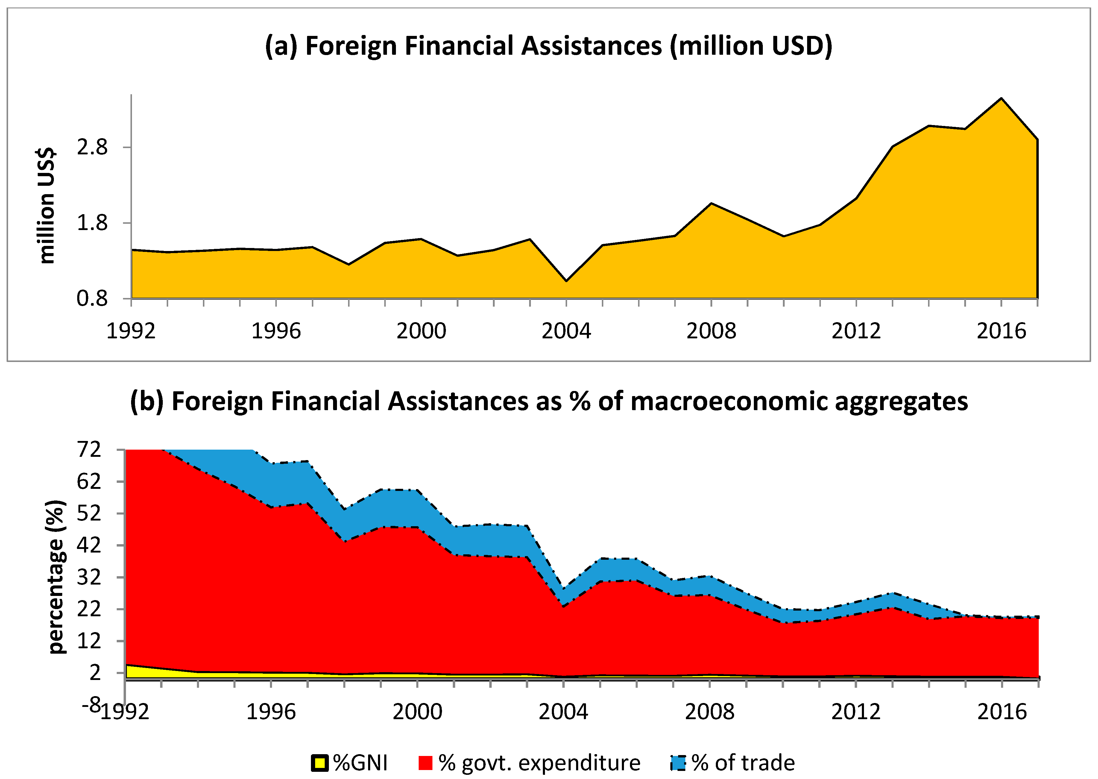
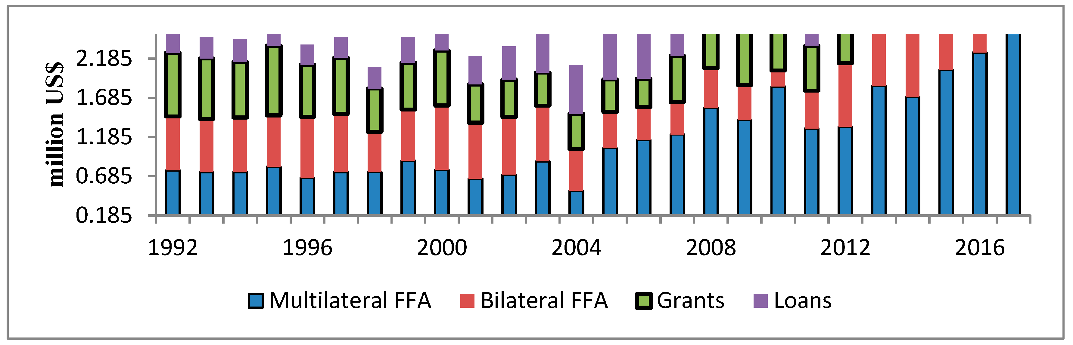
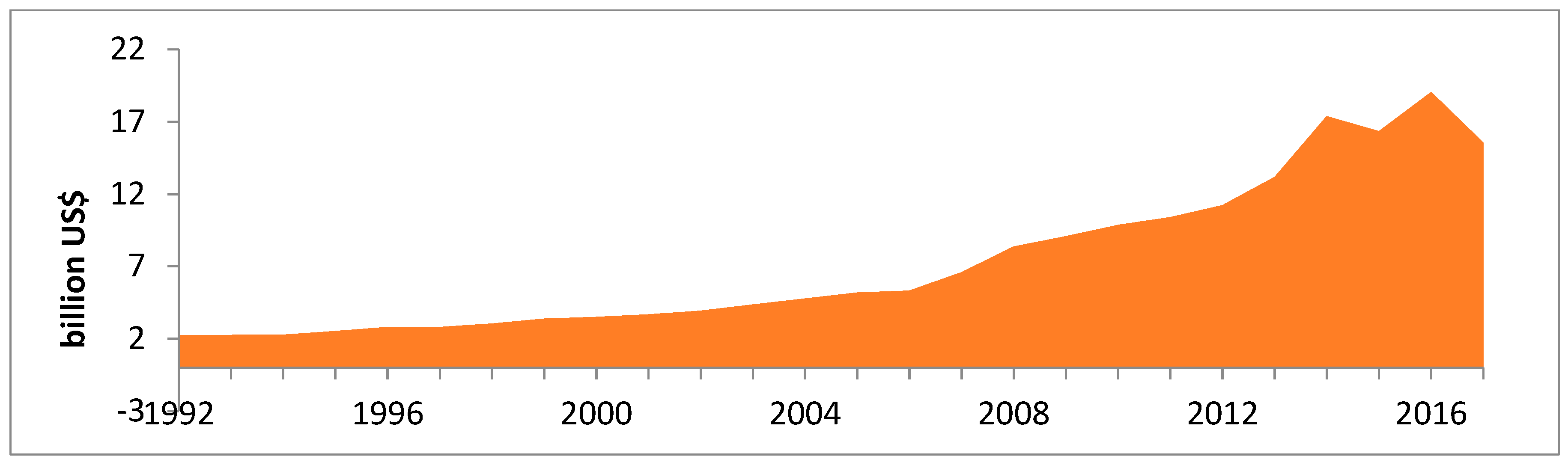
2. An Overview of the FFA and Fiscal Trends in Bangladesh

Ever since the nation’s independence in 1971, the inflow of bilateral and multilateral FFA has played a significant role in the restoration of the war-affected economy of Bangladesh, particularly developing its health and education sectors. Although the total volume of FFA, comprising mainly of grants and concessional loans, flowing into the economy has increased over the years, the nation’s dependence on such foreign assistance has eased with time. Figure 1 illustrates the trends in FFA inflows in Bangladesh between 1992–2017. A closer look into the figure shows that during this period of 26 years, the total amount of FFA received by Bangladesh surmounted to almost 48 billion US dollars (USD). The total figures of FFA peaked at around 3.5 billion USD in 2016, while Bangladesh received the lowest amount of FFA worth 1.03 billion USD in 2004. Although there had been some temporary drops to the inflows, the adverse shocks did not sustain, which is evident from the overall rising trend in the country’s FFA inflows. As far as the dependence on external public finance is concerned, the latter part of Figure 1 depicts that the nation’s reliance on FFA as the major source of foreign currency has declined over the years. The declining trend in the nation’s FFA dependence can be perceived from the downward-sloping curves, expressing total FFA inflows as percentages of gross national income per capita (GNI), total government expenditure, and total trade volumes. For instance, FFA inflows respectively accounted for almost 5%, 70%, and 14% of the nation’s GNI, government expenditure, and trade in the early 1990s, which staggeringly reduced to around 0.6%, 19%, and 0.5%, respectively, by the end of 2017. A plausible explanation behind these trends can be provided by the fact that FFA, unlike the early stages of post-independence, no longer held the lion’s share of the nation’s sources of foreign exchange due to remittances and readymade garments’ export receipts heavily outpacing the total volume of FFA inflows into Bangladesh.
Figure 2 portrays the disaggregated illustrations of total FFA inflows into Bangladesh between 1992–2017. A deeper look into the figure reveals that in the early 1990s, the volumes of FFA originating from the bilateral and multilateral sources were almost identical; however, as time progressed, the relative shares of FFA coming from multilateral donor agencies in the total FFA inflows in Bangladesh have gradually gone up, while the corresponding shares of FFA originating from the bilateral sources have significantly shrunk. This can be understood from both multilateral and bilateral FFA accounting for equal shares in the total FFA inflows, which did not sustain. By the end of 2017, multilateral FFA accounted for almost 86% of total FFA inflows in the country, while only 14% of total FFA was originated from the bilateral sources. However, this is a good transition from the perspective of the overall development of the Bangladesh economy, since bilateral aids, more often than not, tend to be politically motivated which, unlike multilateral aids, are not directly aimed at poverty alleviation and economic development within the recipient economies (Hasan 2011). On the other hand, as far as the composition of FFA is concerned, it can be seen that in most of the time period prior to 2009, Bangladesh received relatively more FFA in the form of foreign grants as compared to foreign concessional loans. However, this trend got reversed in the post-2009 period, which can be seen in 2017, as grants accounted for merely 23% of total FFA inflows, while concessional loans bagged the lion’s share of around 62% of total FFA flowing into Bangladesh. The reducing trend in total foreign grants extended to Bangladesh can be attributed to the development of the nation, whereby it gradually managed to enhance its per-capita income and in the process, the nation lost its eligibility to receive the foreign grants that are decided in terms of the per-capita income levels of the recipient nations.
Figure 3 presents the graphical trend in Bangladesh government’s annual expenditure in between 1992–2017. A closer look into the figure reveals that the level of public investment in the country has increased over the years, which can be understood from the upward trend in its annual government expenditure figures. It can be seen that total public expenditure was around 2.3 billion USD in 1992, which rose to 15.6 billion USD by the end of 2017, depicting an almost eightfold increase in the nation’s total volume of government expenditure within this reference time period. Moreover, this rising trend can also be perceived from the corresponding rise in the nation’s public expenditure level from almost 5.4% of gross domestic product (GDP) in 1992 to around 14% of GDP in 2017 (BER 2017). Finally, Figure 4 illustrates the composition of the government’s revenue in Bangladesh. The trends projected in Figure 4 indicate that the government of Bangladesh has traditionally been reliant on its non-tax measures for the purpose of revenue generation. This is evident from all throughout 1992 and 2017, in which the total amount of tax revenue of the government was below that of the non-tax revenue, despite total revenues depicting a rising trend. Moreover, the gap between non-tax and tax revenues have also aggravated with time, which tends to suggest the ineffectiveness of the government’s tax efforts in generating public revenues. This can be referred to as one of the factors attributing to the nation’s sustained rise in fiscal deficits, compelling it to be dependent on the inflow of FFA for an external public financing of the deficits.

3. Review of Literature

This section has been divided into two subsections, with the first one providing a theoretical framework of government expenditure responses to external inflow of FFA, while the latter presents a review of the relevant empirical findings documented in the literature.

3.1. Theoretical Framework

The theoretical foundations linking FFA inflows to trends in public expenditure responses can be understood from a set of contradicting hypotheses. For instance, it is hypothesized that FFA inflows have positive impacts on government expenditure trends due to the governments of the underdeveloped nations often being stifled by public revenue constraints. As a result, they turn to the foreign financial sources to bridge their respective fiscal shortfalls. Thus, a positive correlation between the volumes of incoming FFA and public expenditure can be anticipated, whereby the received funds are presumed to augment the expenditure budget of the government (Martins 2009). In line with this hypothesis, Khan and Hoshino (1992) claimed that the inflow of foreign aids stimulated government investment expenditure in selected Asian economies. Similarly, McGillivray and Ouattara (2005) concluded that FFA inflows led to enhancement in government consumption expenditure in Cote d’Ivoire. Dinku (2009) argued that foreign aids flowing into Ethiopia stimulated significant increments in the government’s capital expenditure volumes, leveraging the nation’s socioeconomic development targets. Thus, this particular hypothesis tends to advocate in favor of ensuring appropriate efficacies of the FFA extended to the underdeveloped nations in particular.
In contrast, FFA inflows are also presumed to exert public expenditure-dampening impacts within the recipient nations, resulting in a negative correlation between FFA and the volume of public expenditure that follows. A particular reason behind the ineffectiveness of the FFA to relieve the developing economies from their indigenous financial constraints could be understood from the concept of the ‘public moral hazard problem’. In such a circumstance, the inflow of FFA can be associated with levels of public expenditure lower what the recipient governments would have expended had the external financial supports not been extended. Such undesirable actions by the government compromise the efficacies of the FFA, resulting in the foreign funds being fungible (Zampelli 1986; Devarajan and Swaroop 2000). Apart from the FFA inflows adversely affecting public expenditure levels directly, different studies have highlighted the indirect channels through which a negative association between FFA inflows and public expenditure responses can be expected. External financing is said to mitigate domestic taxation efforts whereby revenue generation for the government becomes cumbersome, while the relative dependence on foreign funds tend to grow simultaneously (Thornton 2014). Similarly, Pivovarsky et al. (2003) affirmed that the extension of foreign grants lead to lower domestic revenue mobilization. Moreover, FFA inflows can also go on to accumulate the domestic debt-servicing burdens, leading to lower levels of public expenditure (McGillivray and Ouattara 2005; Fosu 2008). Thus, evaluating these indirect channels is pertinent to deriving key policy implications regarding sustainability and the efficacy of the FFA flowing from the developed to the developing economies across the globe. Appendix A provides a conceptual framework in the context of sector-specific aid fungibility within a recipient economy.

3.2. Empirical Findings

The impacts of FFA inflows on the public expenditure responses within the recipient economies are well documented in empirical literature. For instance, in a study by Pack and Pack (1990), the effects of FFA inflows, in the form of foreign aid, on public expenditure trends in Indonesia were analyzed using annual time-series data spanning from 1966 to 1986. The authors used seemingly unrelated regression analyses to draw conclusions on whether the aid inflows attributed to the expansion in the size of the Indonesian government, and also the fungibility of the aids received was analyzed. According to the findings, foreign aids were referred to be effective in promoting public expenditure in the economy, and the aids extended were in general found not to be displaced, thereby providing support to the non-fungibility aspect of the foreign aids. However, the paper did not address the impacts of foreign aids on other fiscal aggregates, which may directly or indirectly influence the government expenditure behaviors in Indonesia. Moreover, the paper was confined to only investigating the correlation between foreign aid inflows and government expenditure, while excluding the possible causal associations between these variables from the empirical analyses.
Although many studies have opined in favor of similar positive impacts of FFA inflows with regard to promoting greater public expenditures within the recipient economies, there is a great deal of ambiguity regarding this association, as other studies have also remarked against FFA inflows stimulating expansionary pressures on government expenditure levels. Table A1 (in Appendix B) provides a brief summary of the empirical literature addressing the FFA inflow–government expenditure nexus.

4. Empirical Models and Data Specification

This paper follows the empirical models employed by Remmer (2004) and Marc (2012) to, in general, express government expenditure as a function of different forms of FFA inflows and other key control variables. The reduced forms of the log–log models considered in the empirical analyses are given by the following equations:
Δ l n G R E t = α + i = 1 k 1 β i Δ l n G R E t 1 + j = 1 k 1 ρ j Δ F F A + m = 1 k 1 ρ m Δ l n   X t m + λ   E C T t 1 + ε 1 t
where Δ represents the difference operator, k − 1 is the one period of reduced lag length, the subscript t refers to the particular time period of the data, λ is the speed of restoration of equilibrium following a deviation from the equilibrium in the previous lag, and ECT is the error-correction term. The dependent variable GRE denotes the government’s revenue expenditure, FFA is the total foreign assistance received, and X denominates a set of control variables. The coefficient attached to FFA, ρ, is the main estimated coefficient of concern, since it not only explains the mode of the government’s expenditure response to the foreign assistance in question, but it also accounts for the corresponding state of fungibility of the foreign assistance. The control variables include the total annual foreign assistance disbursements (TAD), government debt (DEBT) to account for the government’s debt-servicing burden, the growth rate of GDP (GDPG) to proxy for the level of economic growth, the domestic inflationary rate (INF) to proxy for economic stability within the nation, the urban population (UP) to capture the impacts of urbanization, the population growth rate (PGR) to account for the size demography of the economy, the control of corruption (CC) index to proxy for the level of governance, and the political risk index (PRI) to denote the state of political stability within the country. In order to understand the possible disparities in the impacts of various sources and types of the FFA inflows on the corresponding levels of public expenditures, the aggregate FFA variable in model (1) is replaced by the disaggregated measures of FFA, in separate functions, in terms of both (a) bilateral and multilateral sources and (b) grants and concessional loans, as the two types of FFA inflows in Bangladesh. Thus, model (1) can be modified as follows:
Δ l n G R E t = α + i = 1 k 1 β i Δ l n G R E t 1 + j = 1 k 1 ρ j Δ B F F A t 1 + m = 1 k 1 ρ m Δ l n   X t m + λ   E C T t 1 + ε 1 t
Δ l n G R E t = α + i = 1 k 1 β i Δ l n G R E t 1 + j = 1 k 1 ρ j Δ M F F A t 1 + m = 1 k 1 ρ m Δ l n   X t m + λ   E C T t 1 + ε 1 t
Δ l n G R E t = α + i = 1 k 1 β i Δ l n G R E t 1 + j = 1 k 1 ρ j Δ G R N t 1 + m = 1 k 1 ρ m Δ l n   X t m + λ   E C T t 1 + ε 1 t
Δ l n G R E t = α + i = 1 k 1 β i Δ l n G R E t 1 + j = 1 k 1 ρ j Δ L O A N t 1 + m = 1 k 1 ρ m Δ l n   X t m + λ   E C T t 1 + ε 1 t
where BFFA and MFFA refer to bilateral and multilateral financial assistances received, while GRN and LOAN denote the foreign grants and concessional loans received, respectively.
This paper also examines the FFA-government expenditure relationship in the context of the health and education sectors of Bangladesh in order to shed light on the possible sector-specific variations in the aforementioned nexus. Thus, in model (i), the total GRE variable is separately replaced by the level of government expenditures on health and education. All the control variables, except for TAD, which is replaced by the sector-specific disbursement figures of health aid (HAD) and education aid (EAD), are kept unchanged. Hence, the modified version of model (1) can be given by:
Δ l n G H E t = α + i = 1 k 1 β i Δ l n G H E t 1 + j = 1 k 1 ρ j Δ F F A + m = 1 k 1 ρ m Δ l n   X t m + λ   E C T t 1 + ε 1 t
Δ l n G R E t = α + i = 1 k 1 β i Δ l n G R E t 1 + j = 1 k 1 ρ j Δ F F A + m = 1 k 1 ρ m Δ l n   X t m + λ   E C T t 1 + ε 1 t
The understanding of the association between FFA inflow and government expenditure can also be understood from the effects of the inflows on other fiscal aggregates. Thus, this paper also evaluates the movements in the government’s tax revenues, overall revenue generation, and domestic public borrowings, following a rise in the inflow of FFA into the economy. The following models are considered to shed light on the movements in the aforementioned fiscal aggregates:
Δ l n T A X t = α + i = 1 k 1 β i Δ l n   T A X t 1 + j = 1 k 1 ρ j Δ F F A + m = 1 k 1 ρ m Δ l n   Y t m + λ 1 E C T t 1 + ε 1 t
Δ l n R E V t = α + i = 1 k 1 β i Δ l n   R E V t 1 + j = 1 k 1 ρ j Δ F F A + m = 1 k 1 ρ m Δ l n   Y t m + λ 1 E C T t 1 + ε 1 t
Δ l n D B O R t = α + i = 1 k 1 β i Δ l n   D B O R t 1 + j = 1 k 1 ρ j Δ F F A + m = 1 k 1 ρ m Δ l n   Z t m + λ 1 E C T t 1 + ε 1 t
where TAX refers to the tax revenue of the government, which is expected to provide a picture of the government’s taxation efforts following receipts of the external financial funds; the overall revenue generation of the government is denoted by REV, which would also provide insights into the corresponding government’s non-tax revenue generation efforts; and DBOR refers to the domestic public borrowings from local banks and non-bank financial institutions, which enables capturing the government’s relative dependence on external financing for the fiscal budget as compared to its willingness to mobilize the domestic revenue and curb the overall fiscal deficit of the economy. Y and Z are the sets of control variables, which include quite a few of the control variables comprising in X, and some other key variables linked to the movements in the three fiscal aggregates. These comprise of domestic money supply (M2) and gross national income per capita (GNI).
Annual time-series data spanning from 1985 to 2017 is incorporated into the econometric analyses performed in this paper. All the variables, apart from ln CC and ln PRI, are sourced from the Bangladesh Economic Review report prepared by the Ministry of Foreign Affairs of the People’s Republic of Bangladesh (BER 2005, 2010, 2017), while ln CC and ln PRI are retrieved from the Worldwide Governance Indicators website prepared by the World Bank (WGI 2017). This paper resorts to the use of STATA 15 and EViews 9 statistical software for the econometric methodologies discussed in the next section.

5. Methodology

At first, the entire dataset is tested for stationarity using the Augmented Dickey–Fuller (ADF) unit root testing approach. These pre-estimation econometric analyses are followed by the vector error-correction model (VECM) approach to both short and long-run correlative and causal analyses.

5.1. Unit Root and Cointegration Analyses

There are several ways of testing for the presence of a unit root in time-series dataset. However, the popular test for unit roots in time-series data is the ADF test (Dickey and Fuller 1981) that is run based on Equation (11). This equation is a modification of the original Dickey–Fuller test (Dickey and Fuller 1979), and involves augmenting the Dickey–Fuller equation by lagged values of the dependent variable, and thereby ensuring that the error process is residually uncorrelated. The ADF test also captures the possibility that the dependent variable is characterized by a higher order autoregressive process. The unit root tests are followed by the Johansen test for cointegration to detect the presence of cointegrating equations in our regression models. The Johansen (1988) procedure is applied to test for cointegration, which is known to provide a unified framework for the estimation and testing of cointegration relations in the context of vector autoregressive (VAR) error correction models. Johansen (1988) derived two tests for cointegration, namely the trace test and the maximum Eigenvalue test. The trace statistic test evaluates the null hypothesis that there are at most r cointegrating vectors, whereas the maximum Eigenvalue test evaluates the null hypothesis that there are exactly r cointegrating vectors in xt.

5.2. Vector Error-Correction Model Approach
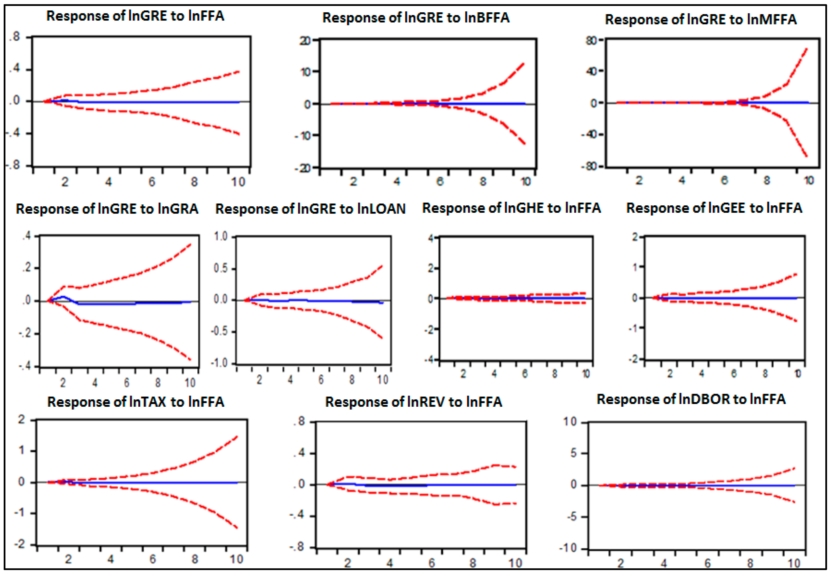
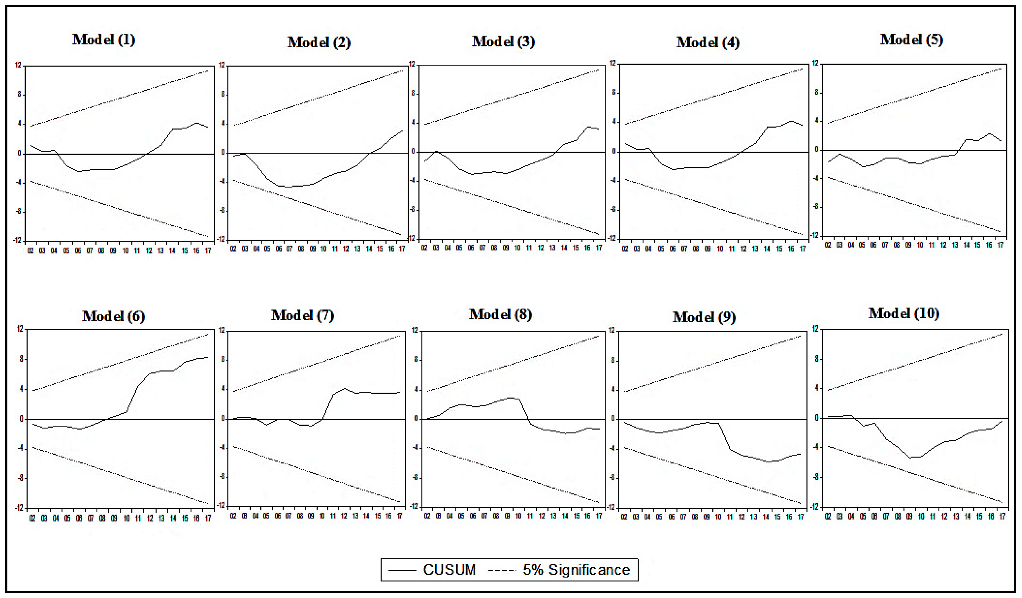
A VECM is a restricted vector autoregressive (VAR) model structured to employ non-stationary series that are known to be cointegrated. It is restricted in the sense that the VECM has cointegrating relations built into the specification so that it restricts the long-run behavior of the endogenous variables to converge to their cointegrating relationships, while allowing for short-run adjustment dynamics. The cointegration term is known as the error-correction term (ECT), which provides the pace at which any deviation from the long-run equilibrium in the previous lag is corrected in the next lag through a series of partial short-run adjustments. This is referred to as the error-correction mechanism.
Engle and Granger (1987) showed that the VECM is an appropriate method to model the long-run as well as the short-run dynamics among the cointegrated variables. However, in the context of a multivariate regression analysis, the VECM approach is preferred to provide only the short-run causality among the variables. Causality inferences in the multivariate framework are made by estimating the parameters of the following VECM equations:
Δ Y = α + i = 1 m β i Δ Y t i + j = 1 n γ j Δ X t j + k = 1 0 δ Δ M s + l = 1 p ζ Δ N + θ Z t 1 + ε t
Δ X = a + i = 1 m b i Δ Y + j = 1 n c j Δ X t j + k = 1 0 d Δ M s + l = 1 p e Δ N + f Z t 1 + ξ t
where Zt−1 is the error-correction term, which is the lagged residual series of the cointegrating vector. The error-correction term measures the deviations of the series from the long-run equilibrium relation. For example, from Equation (11), the null hypothesis that X does not Granger-cause Y is rejected if the set of estimated coefficients on the lagged values of X is jointly significant. Furthermore, in those instances where X appears in the cointegrating relationship, the hypothesis is also supported if the coefficient of the lagged error-correction term is significant. Changes in an independent variable may be interpreted as representing the short-run causal impact, while the error-correction term provides the adjustment of Y and X toward their respective long-run equilibrium. Thus, the VECM representation allows us to differentiate between the short- and long-run dynamic relationships. The chi-square test statistic is used to determine the short-run causalities between pairs of variables in the model.
In the context of a panel of N countries, three regressors (X, Y, and Z) across T time period, the VECM model can be given by:
[ Δ X i t Δ Y i t Δ Z i t ] = [ ω 1 i ω 2 i ω 3 i ] + k = 1 q [ α 11 i k α 12 i k α 13 i k α 21 i k α 22 i k α 23 i k α 31 i k α 32 i k α 33 i k ] [ Δ X i t k Δ Y i t k Δ Z i t k ] + [ γ 1 i γ 2 i γ 3 i ] E C T i t 1 + [ μ 1 i t μ 2 i t μ 3 i t ]
where Δ denotes first difference transformation of the variables. In addition, the variance decomposition and impulse response function analyses are also considered in the analyses to provide robust support to the regression estimates. Finally, the estimated VECMs pass through diagnostic tests in the form of the Lagrange multiplier test for autocorrelation proposed by Breusch and Godfrey (1980), Jarque and Bera’s (1980) test of normality distribution of the residuals, White’s (1980) test of homoscedastic variance, and the cumulative sum of squares test for model stability developed by Page (1954).

6. Results

The ADF unit root test results, which are reported in Table 1, show that all the variables included in the empirical models are stationary at their first differences, which nullifies the possibility of the regression analyses, to be performed later, being spurious. The variables being commonly integrated into order 1 [i.e., I (1)] allows us to proceed to the Johansen test of cointegration.
Table 2 reports the cointegration test results, which confirm the presence of cointegrating equations in all the models. These results provide empirical evidence of long-run associations between the variables in each of the models.
The presence of cointegration among the variables allows us to perform the VECM analysis. The corresponding VECM results for Equations (1)–(5) are reported in Table 3. A closer look into the coefficient estimates provides the initial impression regarding the variations in responses to public expenditures with respect to different measures of FFA inflows. Thus, the decision of disaggregation of the total FFA can be claimed to be a justified one based on the results. The results indicate that FFA inflows as a whole tends to have a dampening effect on the government expenditure responses in Bangladesh as perceived from both the short and long-run negative estimated coefficients attached to lnFFAt and ΔlnFFAt, which are statistically significant at the 1% and 10% levels, respectively. The predicted elasticities suggest that a 1% rise in the inflow of total FFA in Bangladesh tends to stimulate declines in the government’s expenditure levels by 0.46% and 5.51% in the short and long-run respectively, on average ceteris paribus. Thus, these aforementioned findings tend to validate the hypothesis of a negative correlationship between FFA inflows and total public spending levels in Bangladesh. These results corroborate to the findings Thamae and Kolobe (2016) for Lesotho, while contradicting the findings by Bwire et al. (2013) for Rwanda.
A plausible explanation behind this crowding-out effect of external public financial inflows could be that a rise in the inflows, synonymous to an aggravation in the government’s debt burdens, could well force the government to reallocate the external funds to service the existing debts rather than investing them within the productive sectors of the economy. Similar debt-servicing responses to FFA inflows have been concluded in the study by Pack and Pack (1993). This claim is supported by the statistically significant and negative long-run coefficient attached to lnDEBTt implying a negative association between debt-servicing burdens and public revenue expenditures in Bangladesh.
These results also advocate in favor of FFA inflows originating from bilateral sources exerting similar adverse impacts on the government’s expenditure allocations. However, on the other hand, the statistically significant positive estimates of the long-run coefficients attached to ln MFFAt and ln LOANt assert that such foreign inflows rather enhance public investment for Bangladesh. Thus, in the case of the FFA in the form of loans, the hypothesis of a positive correlation between FFA and public expenditure responses is affirmed. On the other hand, inflows of foreign grants are found to be statistically insignificant for explaining the variations in government expenditure trends, which imposes a concern regarding the future extension of grants to Bangladesh. The reason behind foreign concessional loans having positive impacts on government expenditure, as opposed to the impacts of grants, can be understood from the notion that these loans usually come with the conditionality of being expended, as imposed by the donors.
Besides, the other relevant findings reported in Table 3 also suggest that disbursement of the FFA is imperative with respect to enhancing the public expenditure levels in Bangladesh. The positive association between such disbursements and government expenditure, in light of the estimated coefficients attached to ln TADt, validates this claim, which can also explain the earlier findings regarding the potential crowding out of public expenditure following the inflow of FFA. This is a realistic finding in the context of Bangladesh, since the nation has traditionally exhibited poor aid-disbursement trends resulting in the piling up of the unutilized foreign exchange reserves (Bhattacharya et al. 2005).
Furthermore, the VECM results presented in Table 3 also highlight the importance of controlling for corruption within the economy as a means to channel the external funds to investment in public projects. This is evident from the positive estimates of most of the coefficients attached to ln CCt, which imply that a reduction in the incidence of corruption could stimulate public investments in Bangladesh. Finally, the negative and statistically significant error-correction terms reported in this table suggest that deviations from the long-term equilibrium are corrected at rates of 7%, 134%, and 117% in the following year, in the context of models (1), (2), and (3), respectively. For Equations (4) and (5), the ECT are not statistically significant, which raises concerns regarding the pace of the error-correction mechanism for these models.
The concept of aid fungibility is crucial from the sustainability of the FFA inflows. In the same vein, for a robustness check of the aforementioned results, this paper also aimed to evaluate the fungibility of the incoming sector-specific FFA in Bangladesh. The relevant results from the VECM analyses are reported in Table 4. The results indicate contrasting effects of FFA inflows on government expenditure levels within the health and education sectors of Bangladesh. A deeper look into the estimated coefficients reveals that FFA inflows restrain government expenditure in the health sector, thus validating the hypothesis of a negative FFA–government expenditure nexus. This is evident from the negative and statistically significant coefficients attached to ln FFAt and ΔFFAt in the context of model (4). These estimates imply that, holding all else constant, a 1% rise in FFA inflows into Bangladesh is associated with 1.19% and 0.90% deteriorations, on average, in short and long-run public health expenditure figures, respectively. Hence, it can be said that the FFAs directed at Bangladesh’s health sector are fungible to some extent. This particular finding is of paramount relevance for a developing economy such as Bangladesh, since the per-capita public investments in the national health sector have been pretty scant in recent times (Chaity 2018).
In contrast to the health sector findings, the corresponding results in Table 4 show that utilization of the foreign assistances aimed at Bangladesh’s education sector has been comparatively better. The positive and statistically significant short and long-run coefficients attached to ln FFAt and Δln FFAt, in line with the hypothesis of a positive interlinkage between FFA and government expenditure, in the context of model (7), provide statistical evidence to this statement. It is found that a 1% enhancement in the volume of FFA inflows in the country is linked to increments in the volumes of public expenditure on education by 0.50% in the short run and 1.25% in the long run, on average ceteris paribus. These results also imply that the foreign educational assistances extended to the government of Bangladesh, although being partially fungible in the short run, are non-fungible in the long run, since the estimated long-run coefficient attached to ln FFAt is more than 1, providing statistical support to the non-fungibility aspect. This is inspiring for the Bangladesh economy, as the non-fungibility nature of the FFA inflows directed at the education sector enhances the future prospects of human capital development. However, despite the non-fungibility of the educational FFA, the small value of the coefficient attached to ln FFAt presses the need for the government to further raise budgetary allocations for the education sector, which at present is way below par (Habib 2018).
Apart from the government expenditure responses to FFA inflows, the responses of the other key fiscal aggregates to these external inflows are also important to shed light on the FFA inflow–government expenditure nexus. Against this backdrop, the effects of external public financing on Bangladesh’s taxation efforts, revenue generation, and domestic public borrowings have also been evaluated. The corresponding estimated short and long-run coefficients in the context of models (8), (9), and (10) are reported in Table 5. In general, the estimated elasticities advocate in favor of FFA inflows stimulating dampening impacts on the government’s tax and non-tax efforts, as perceived from the negative and statistically significant long coefficients attached to ln TAXt and ln REVt, respectively. The results indicate that a 1% rise in the total inflows of FFA in Bangladesh is accompanied by declines in the government’s tax and total revenues by 1.82% and 7.059%, respectively, on average ceteris paribus. Similar conclusions are made by Franco-Rodriguez et al. (1998) in the context of Pakistan.
Moreover, the fact that the FFA inflow elasticity of total revenue generation in Bangladesh is pretty low explicitly points toward the nation’s relative reliance on external sources of finance for bridging the persistent fiscal deficit in the country. These findings affirm the government’s ineffectiveness in mobilizing its domestic revenues. The negative association between tax revenue and external public financing can be tapped to explain the lion’s share of non-tax revenues in total revenue collection in Bangladesh (Murshed and Saadat 2018). On the other hand, the estimated results also reveal a negative association between FFA inflows and domestic public borrowings, since a 1% rise in FFA inflows is found to reduce the total amount of domestic borrowings by the government by 0.52% on average in the short run, ceteris paribus. However, although this particular finding is ideal from the sense that the possibility of public borrowing from the local banks and non-bank financial institutions attributing to the crowding out of private investments within the economy is slim, this negative association further highlights the relative FFA dependence of the nation.
The VECM analyses are followed by the variance decomposition and impulse response functions analyses, for a further robustness check of the findings. Thus, the variance decomposition analyses are done over a span of 10 years, and the results are illustrated in Table 6 and Table 7. Table 6 reports the outputs in the context of models (1), (2), (3), (4), (5), (6), and (7), which also provides an understanding of the trends in the public expenditure responses to FFA inflows in Bangladesh. According to the estimates, it can be seen that an exogenous shock to FFA inflows result in merely 4.22% variation in the forecast error variance (FEV) of government expenditure levels. However, upon the disaggregation of total FFA inflows, it is found that at the 10th period, shocks to bilateral FFA, multilateral FFA, grants, and concessional loans contributed to 2.10%, 8.91%, 8.49%, and 7.80% variations, respectively, in the government expenditure values. Such low explanatory powers of the disaggregated measures of FFA inflows in explaining the total variation in the aggregate public spending responses in Bangladesh imply that the government’s expenditure responses to FFA inflows are subject to extended lags. Moreover, the findings from the variance decomposition analyses also points toward the debt-servicing burden of the government being closely associated with the public expenditure responses.
Furthermore, the results from the variance decomposition analyses also show that exogenous shocks to FFA inflows tend to explain merely a little over 3% of the variations in the FEV of public expenditure levels, at the 10th period, in both the health and education sectors of Bangladesh. Another important takeaway from the variance decomposition analyses is that exogenous shocks to the rate of urbanization within the country explains around 22.03% and 18.81% of the variations in the FEVs of public health and education expenditures, which implies that as more people travel to the urban areas, the adversities associated with the unplanned urbanization woes of Bangladesh are somewhat marginalized via changes in the fiscal allocations in the health and education sectors.
Table 7 reports the results from the variance decomposition analyses in the context of models (8), (9), and (10). A close look into the estimates reveals that FFA inflow shocks in Bangladesh account for merely 7.31%, 5.98%, and 3% of the variations in the FEVs of tax revenues, total revenues, and domestic public borrowings, respectively. These once again points toward FFA inflows being effective in affecting these three fiscal aggregates for an extended period of time. Finally, it is also seen that shocks to corruption control incidences and domestic inflationary pressures also explain a great deal of variations in the government’s tax and total revenue volumes, which—in line with the corresponding elasticities from the VECM analyses—tend to indicate toward ensuring good governance and economic stability with respect to increasing public revenues in Bangladesh.
The variance decomposition analyses are followed by the IRF exercises. Figure 5 illustrates the impulse response graphs in which only the lagged responses of government expenditures and the other three fiscal aggregates to standard deviation impulses (shocks) to FFA inflows, over a period of 10 years, are reported. According to the IRFs, it can be seen that one standard deviation impulses to all the aggregate and disaggregate measures of FFA inflows in Bangladesh, in general, have nominal impacts on the corresponding government expenditure responses, almost all throughout the 10-year period. A closer look into the IRFs reveal that a one-time standard deviation impulse to the overall FFA inflow in the country has a nominal positive impact on government expenditure up to two years, after which the effect decays down to zero. This implies that external financing contributes to greater public expenditure in the short run; however, the effect does not seem to sustain over the long run. Moreover, standard deviation impulse to international grants is found to exert fluctuating impacts on government spending. The corresponding IRF graph illustrates that any positive standard impulse to grants has a positive impact on government expenditure for about 2.5 years, but the effect becomes negative from then after, and is sustained almost all throughout the remaining periods. Therefore, this finding seems to question the fungibility of the foreign grants extended to Bangladesh, and also highlights the public investment-dampening effects attached to such foreign inflows. Furthermore, it is also found that standard deviation impulses to FFA inflows do not stimulate any impact on the government’s expenditure responses in both the health and education sectors all throughout the 10-year period of analysis. Hence, these results have key policy implications with regard to structuring appropriate public policies to channel the FFA to the health and education sectors in the form of public investments.
In order to understand the causal associations between FFA inflows and the corresponding public expenditure responses, this paper also examines the VECM Granger causality analyses in the context of all the 10 models. Table 8 reports only the short and long-run causalities between the FFA inflows and the associated responses of public spending figures in Bangladesh in the context of models (1) to (7). According to the findings, there is statistical evidence regarding FFA inflows influencing changes in government expenditures in Bangladesh, both in the short and long runs, as perceived from the unidirectional causalities found to be stemming from ln FFAt to ln GREt over both the time horizons. This implies that external public financing, as a whole, does attribute to the expenditure decision making of the government. However, there is no statistical evidence suggesting the reverse causation, which can be interpreted as FFA provided to the Bangladesh government not entirely depending on the extent of utilization of the funds extended. On the other hand, taking the disaggregated measures of FFA inflows into consideration, the Granger causality test results indicate toward unidirectional causalities running from both bilateral and multilateral FFA to government expenditure in both the short and long runs. In addition, a reverse causality running from government expenditures to bilateral FFA inflows was also found to exist in the long run. Thus, this bidirectional causal association implies that the prospects of future FFA extensions by foreign countries to Bangladesh do hinge on the proper utilization and non-fungibility of the assistive funds. Furthermore, the results also suggest that FFA inflows influence the government expenditure on education, which is not the case in the context of the health sector of the economy. This is a key finding, in the sense that the inability of the FFA inflows with regard to augmenting the government’s public expenditure allocations for the education sector is a threat to the nation’s future prospects of human capacity development, provided the fiscal allocations for this sector are reducing with time. Apart from these, the results from the causality analyses also provide statistical evidence regarding the long-run influences of FFA inflows on the government’s total revenue generation; however, no causal association was found to exist between FFA inflows and tax revenue generation and domestic public borrowings. The unidirectional causality running from FFA inflows to total public revenue generations, along with the negative associations between these variables found from the VECM analyses, implies that a rise in the volume of external public financing does exhibit a reduction in the government’s efforts to mobilize domestic revenue, which is synonymous with an aggravation in the nation’s relative dependence on foreign sources of public finance.
Table 9 reports the statistical estimates from the Breusch–Godfrey Lagrange multiplier, the Jarque-Bera normality and White heteroscedasticity test results. In general, the results refer to all the regression models being free from serial correlation, the corresponding residuals being normally distributed, and the absence of heteroscedasticity within the models.
Figure 6 illustrates the plots of the Cumulative Sum (CUSUSM) tests, and the associated charts tend to affirm the stability of the regression models, as the residuals are found to be within the 95% confidence interval.

7. Conclusions

Scant amounts of public revenue have always resulted in fiscal deficits among the developing countries in particular, thus compelling these nations to being largely reliant on external financing of the proposed expenditure budgets. Thus, the inflows of external funds can be associated with the public spending responses within the recipient economies. Against this backdrop, this paper tried to shed light on the dynamic relationships between public expenditure movements within the economy of Bangladesh following the inflows of both aggregate and disaggregated volumes of FFA.
According to the statistical evidences found in this paper, it can be generally concluded that external financing of the fiscal deficits in Bangladesh, in general, triggers a crowing-out effect on the nation’s total public expenditures. This negative association between FFA inflows and the corresponding size of the government tends to indicate toward a public moral hazard problem. Thus, the government is somewhat reluctant to expend its domestic revenue to the extent that it would have naturally spent if the foreign assistances had not been received. Nevertheless, the financial assistances from multilateral donor agencies and concessional foreign loans extended to Bangladesh were found to be trigger expansion of the government’s expenditure volumes. This, to some extent, is impressive with regard to the proper utilization of these assistive funds. Although similar public expenditure responses were in the context of the education sector of Bangladesh, public health expenditure responses to income FFAs were found to reduce the corresponding budgetary allocations aimed at the development of the health sector. Thus, these results pointed toward a relative preference of the Bangladesh government in terms financing public projects in the education sector while the reducing health sector public investments. Therefore, it can be said that the health aids flowing into Bangladesh are fungible in nature.
Hence, if Bangladesh targets to fulfill its commitment to achieving the sustainable development goals by 2030, and simultaneously attain its national goals of becoming a lower middle-income and a upper middle-income economy by 2021 and 2041 respectively, it has to resolve the public investment-dampening effects associated with the external financing of its fiscal shortfalls. Moreover, it is ideal to gradually lessen the nation’s dependence on foreign finance and rather aim to enhance the rate of mobilization of the domestic public revenues. In particular, stern steps have to be undertaken to curb the tendency of tax evasion in the public through the provision of appropriate incentives.
A possible solution to all the fiscal problems associated with external budget financing in the context of Bangladesh could be in terms of the government’s willingness to promote good governance within the economy which, in line with the findings from the empirical analyses performed in this paper, could ideally ensure the proper utilization of the FFA inflows and thereby augment the total public expenditure volumes, which in turn would ultimately drive away the nation’s reliance on foreign funds and ensure greater self-sufficiency in both the generation and mobilization of domestic revenues.
The limitations faced in this paper were in the form of data constraints, which restrained the incorporation of crucial explanatory variables into the empirical models. Moreover, the unavailability of sector-specific FFA and public expenditure data also confined the sectoral FFA–public expenditure response analyses to only the health and the education sector. As part of the future scope of research, this paper can be a standpoint in undertaking further investigations regarding the factors affecting the relative aid dependence in Bangladesh, and also shed light on the other factors attributing to the public investment crowding-out impacts of external financing. Moreover, panel econometric tools can be applied to perform regional studies, which can add to the robustness of the results found in this paper.

Funding

The research received no external funding.

Conflicts of Interest

The author declares no conflict of interest.

Appendix A

Aid Fungibility: The nexus between government expenditure and inflow of FFA can also be evaluated in light of the fungibility analysis of the inward foreign funds. Suppose that there is a small developing economy that has experienced sustained fiscal deficits in the past. For simplicity, let us assume that there are only two sectors within this economy: health and education, where both these sectors play key roles in the overall development of the economy. Moreover, it is also assumed that the government invests in both these sectors via its own domestic revenue, as well as via the FFA extended by the foreign donors. Now, suppose that the government receives a certain amount of foreign health grant (G), which is conditional to be exhausted in the health sector. Thus, the impact of this inward grant on the public expenditure allocations within the recipient economy can be evaluated in terms of the fungibility of the grant. Figure A1 illustrates the possible modes of government expenditure responses to the health grant received. The pre-grant budget constraint faced by the government is given by B0B0, and is based on the initial preference of the government (U0) for the optimal public expenditure allocation, as indicated by point A on the figure, in which the health and education sectors are given by H0 and E0, respectively. A point to note here is that these allocations are solely financed by the government’s own domestic revenue. Following the inflow of the health grant, there is an outward shift in the budget constraint graph, whereby the post-grant budget constraint is given by B1B1. The fungibility of the health grant can take two forms.
Figure A1. Fungibility of FFA and Public Expenditure Responses. Source: Author’s own.
Economies 07 00095 g0a1
In the case of the health grant being fungible, the post-grant optimal choice of public expenditure in the health and education sectors is an interior solution at point A. However, the economy would eventually shift to a new optimal point B in order to reach a higher preference (U1). At this point, the new levels of public expenditure in the health and education sectors are H1 and E1, respectively, which are higher than the corresponding pre-grant levels. In this case, that the level public expenditure in the education sector has gone up reflects the partial fungibility of the health grant, whereby a portion of the FFA directed at the health sector has been displaced and invested in the education sector. Thus, the health grant in this aspect has generated a dampening effect on public health expenditure, although enhancing the overall level of public expenditure within the economy. On the other hand, in the case of the health grant being non-fungible, the new mix of public expenditure would be given by point C, whereby the level of public expenditure in the health sector would go up by exactly the amount of health grant received (H2), while leaving the corresponding public expenditure level in the education sector unaltered. Thus, in this scenario, the inflow of the health grant stimulates public expenditure within the health sector as well as increases the overall level of public expenditure within the economy. The figure also shows that the proper utilization of the FFA is welfare maximizing for the recipient economy, which can be perceived from point C being on the highest possible preference curve of the government subject to the budget constraint faced.

Appendix B

Table A1. An Overview of the Empirical Literature on the FFA Inflow–Government Expenditure Nexus. VAR: vector autoregressive.
StudyEstimation MethodPeriodCountriesResults
Pack and Pack (1993)Seemingly unrelated regression estimator1968–1986Dominican RepublicForeign assistances intended for development expenditure are displaced to fiscal-deficit reduction and debt servicing.
Franco-Rodriguez et al. (1998)Non-linear three-stage least squares estimator 1956–1995PakistanOnly about 50% of total aid inflows have augmented total government consumption in Pakistan. An increase in foreign aid inflow is associated with a positive impact on government expenditure and a negative impact on the tax revenues.
Mavrotas (2002)Non-linear three-stage least squares estimator 1973–1992India (1973–1990)
Kenya (1973–1992)
Project aids flowing into India are found to be less fungible compared to program aids. Similarly, the fungibility of aid inflows to Kenya depends on the type of the aid.
Osei et al. (2005)VAR, VECM, and impulse response functions1966–1988GhanaNo direct impact of foreign aid inflows on public expenditure in the short run. The inflows are found to affect domestic public borrowing and tax revenues negatively and positively, respectively.
McGillivray and Ouattara (2005)ARDL cointegration approach, non-linear three-stage least squares estimator 1975–1999Cote d’IvoireGovernment expenditure does not increase following inward flows of foreign aids. Most of the aid is utilized for debt servicing, and foreign aid inflows attribute to rising public debts.
Bhattarai (2007)Johansen cointegration and generalized impulse response analyses1975–2002NepalForeign aid positively affects both development and non-development expenditure. Development aid is found to be fungible due to it being displaced to the non-development expenditure of the government.
Martins (2007)Non-linear three-stage leastsquares estimator 1964–2005EthiopiaForeign aid positively affects government investment. Foreign loans have a stronger impact on public expenditure than grants. Foreign aid reduces domestic public borrowing and displaces public revenues.
Bwire et al. (2013)Cointegrated VAR analysis1972–2008UgandaForeign aids increase government expenditure and raise the tax efforts as well.
Thamae and Kolobe (2016)Johansen cointegration analysis and Granger causality tests1982–2010LesothoA rise in the inflow of foreign aids results in adverse impacts on recurrent expenditure while increasing the capital expenditure of the government. Thus, foreign aid inflows are referred to be non-fungible in nature. A unidirectional long-run causal association stemming from foreign aid to recurrent public expenditure is found.
Bwire et al. (2017)Cointegrated VAR analysis1990Q1–2015Q4RwandaForeign aid inflows increase public expenditure and tax revenues while reducing public borrowings from domestic sources

References

  1. Amin, Sakib Bin, and Muntasir Murshed. 2018a. An Empirical Investigation of Foreign Aid and Dutch Disease in Bangladesh. The Journal of Developing Areas 52: 169–82. [Google Scholar] [CrossRef]
  2. Amin, Sakib Bin, and Muntasir Murshed. 2018b. A Cross-Country Investigation of Foreign Aid and Dutch Disease: Evidence from selected SAARC Countries. Journal of Accounting, Finance and Economics 8: 40–58. [Google Scholar]
  3. BER. 2005. Bangladesh Economic Review. Dhaka: Ministry of Foreign Affairs, People’s Republic of Bangladesh. [Google Scholar]
  4. BER. 2010. Bangladesh Economic Review. Dhaka: Ministry of Foreign Affairs, People’s Republic of Bangladesh. [Google Scholar]
  5. BER. 2017. Bangladesh Economic Review. Dhaka: Ministry of Foreign Affairs, People’s Republic of Bangladesh. [Google Scholar]
  6. Bhattacharya, Debapriya, M. Syeed Ahamed, Wasel Bin Shadat, and Md. Masum Billah. 2005. State of the Bangladesh Economy in FY2003−04. Independent Review of Bangladesh’s Development. Centre for Policy Dialogue, Bangladesh. Available online: https://www.cpd.org.bd/downloads/IRBD/SecInt_IRBD2005.pdf (accessed on 29 June 2018).
  7. Bhattarai, Badri Prasad. 2007. Foreign aid and government’s fiscal behaviour in Nepal: An empirical analysis. Economic Analysis and Policy 37: 41–60. [Google Scholar] [CrossRef]
  8. Bräutigam, Deborah. 2011. Aid ‘with Chinese characteristics’: Chinese foreign aid and development finance meet the OECD-DAC aid regime. Journal of International Development 23: 752–64. [Google Scholar] [CrossRef]
  9. Bräutigam, Deborah A., and Stephen Knack. 2004. Foreign aid, institutions, and governance in sub-Saharan Africa. Economic Development and Cultural Change 52: 255–85. [Google Scholar] [CrossRef]
  10. Breusch, Trevor S., and Lesley G. Godfrey. 1980. A Review of Recent Work on Testing for Autocorrelation in Dynamic Economic Models. Southampton: University of Southampton. [Google Scholar]
  11. Bwire, Thomas, Oliver Morrissey, and Tim Lloyd. 2013. A Timeseries Analysis of the Impact of Foreign Aid on Central Government’s Fiscal Budget in Uganda. WIDER Working Paper No. 2013/101. Helsinki: World Institute for Development Economics Research (UNU-WIDER), United Nations University. [Google Scholar]
  12. Bwire, Thomas, Caleb Tamwesigire, and Pascal Munyankindi. 2017. Fiscal Effects of Aid in Rwanda. In Studies on Economic Development and Growth in Selected African Countries. Singapore: Springer, pp. 79–101. [Google Scholar]
  13. Chaity, Afroz Jahan. 2018. Budget Allocations for Health, Education Continue to Shrink. Dhaka Tribune. Available online: https://www.dhakatribune.com/bangladesh/2018/06/29/budget-allocations-for-health-education-continue-to-shrink (accessed on 29 June 2018).
  14. Chenery, Hollis B., and Alan M. Strout. 1966. Foreign assistance and economic development. The American Economic Review 56: 679–733. [Google Scholar]
  15. Devarajan, Shantayanan, and Vinaya Swaroop. 2000. The implications of foreign aid fungibility for development assistance. In The World Bank: Structure and Policies. Cambridge: Cambridge University Press, pp. 196–209. [Google Scholar] [Green Version]
  16. Dickey, David A., and Wayne A. Fuller. 1979. Distribution of the estimators for autoregressive time series with a unit root. Journal of the American Statistical Association 74: 427–31. [Google Scholar]
  17. Dickey, David A., and Wayne A. Fuller. 1981. Likelihood ratio statistics for autoregressive time series with a unit root. Econometrica: Journal of the Econometric Society 49: 1057–72. [Google Scholar] [CrossRef]
  18. Dinku, Yonatan Minuye. 2009. The Impact of Foreign Aid on Government Fiscal Behaviour: Evidence from Ethiopia. Ph.D. thesis, University of the Western Cape, Cape Town, South Africa. Available online: http://etd.uwc.ac.za/handle/11394/2701 (accessed on 29 June 2018).
  19. Engle, Robert F., and Clive W. J. Granger. 1987. Co-integration and error correction: Representation, estimation, and testing. Econometrica: Journal of the Econometric Society 55: 251–76. [Google Scholar] [CrossRef]
  20. Feeny, Simon. 2003. The impact of foreign aid on poverty and human well-being in Papua New Guinea. Asia Pacific Development Journal 10: 73–93. [Google Scholar] [CrossRef]
  21. Feyzioglu, Tarhan, Vinaya Swaroop, and Min Zhu. 1996. Foreign Aid’s Impact on Public Spending. No. 1610. Washington, DC: The World Bank. [Google Scholar]
  22. Fosu, Augustin Kwasi. 2008. Implications of the external debt-servicing constraint for public health expenditure in sub-Saharan Africa. Oxford Development Studies 36: 363–77. [Google Scholar] [CrossRef]
  23. Franco-Rodriguez, Susana, Oliver Morrissey, and Mark McGillivray. 1998. Aid and the public sector in Pakistan: Evidence with endogenous aid. World Development 26: 1241–50. [Google Scholar] [CrossRef]
  24. Gbesemete, Kwame P., and Ulf-G. Gerdtham. 1992. Determinants of health care expenditure in Africa: A cross-sectional study. World Development 20: 303–8. [Google Scholar] [CrossRef]
  25. Griffin, Keith. 1970. Foreign capital, domestic savings and economic development. Bulletin of the Oxford University Institute of Economics & Statistics 32: 99–112. [Google Scholar]
  26. Habib, Wasim Bin. 2018. Education lacks due attention. The Daily Star. June 8. Available online: https://www.thedailystar.net/frontpage/bangladesh-national-budget-2018-19-education-outlay-not-enough-1588219 (accessed on 28 May 2019).
  27. Hasan, Md Didarul. 2011. Foreign Aid Dependency of Bangladesh: An Evaluation. The Chittagong University Journal of Business Administration 26: 281–94. [Google Scholar]
  28. Jarque, Carlos M., and Anil K. Bera. 1980. Efficient tests for normality, homoscedasticity and serial independence of regression residuals. Economics Letters 6: 255–59. [Google Scholar] [CrossRef]
  29. Johansen, Søren. 1988. Statistical analysis of cointegration vectors. Journal of Economic Dynamics and Control 12: 231–54. [Google Scholar] [CrossRef]
  30. Khan, Haider Ali, and Eiichi Hoshino. 1992. Impact of foreign aid on the fiscal behavior of LDC governments. World Development 10: 1481–88. [Google Scholar] [CrossRef]
  31. Lancaster, Carol. 1999. Aid effectiveness in Africa: The unfinished agenda. Journal of African Economies 8: 487–503. [Google Scholar] [CrossRef]
  32. Lancaster, Carol. 2008. Foreign Aid: Diplomacy, Development, Domestic Politics. Chicago: University of Chicago Press. [Google Scholar]
  33. Marc, Lukasz. 2012. New Evidence on Fungibility at the Aggregate Level. No. 12−083/2. Amsterdam: Tinbergen Institute. [Google Scholar]
  34. Martins, Pedro. 2007. The Fiscal Impact of Aid Flows: Evidence from Ethiopia. No. 43. Brasilia: International Policy Centre for Inclusive Growth. [Google Scholar]
  35. Martins, Pedro M. G. 2009. The impact of foreign aid on government spending, revenue and domestic borrowing in Ethiopia. In Economic Alternatives for Growth, Employment and Poverty Reduction. London: Palgrave Macmillan, pp. 100–36. [Google Scholar]
  36. Masud, Nadia, and Boriana Yontcheva. 2005. Does Foreign aid Reduce Poverty? Empirical Evidence from Nongovernmental and Bilateral Aid. Washington, DC: International Monetary Fund. [Google Scholar]
  37. Mavrotas, George. 2002. Foreign aid and fiscal response: Does aid disaggregation matter? Weltwirtschaftliches Archiv 138: 534–59. [Google Scholar] [CrossRef]
  38. McGillivray, Mark. 1989. The allocation of aid among developing countries: A multi-donor analysis using a per capita aid index. World Development 17: 561–68. [Google Scholar] [CrossRef]
  39. McGillivray, Mark, and Oliver Morrissey. 2001. A Review of Evidence on the Fiscal Effects of Aid. CREDIT Working Paper No. 01/13. Nottingham: Centre for Research in Economic Development and International Trade. [Google Scholar]
  40. McGillivray, Mark, and Bazoumana Ouattara. 2005. Aid, debt burden and government fiscal behaviour in Cote d’Ivoire. Journal of African Economies 14: 247–69. [Google Scholar] [CrossRef]
  41. Murshed, Muntasir. 2018. The Harberger-Laursen-Metzler Effect and Dutch Disease Problem: Evidence from South and Southeast Asia. Journal of Accounting, Finance and Economics 8: 134–66. [Google Scholar]
  42. Murshed, Murshed, and Syed Y. Saadat. 2018. Modeling Tax Evasion across South Asia: Evidence from Bangladesh, India, Pakistan, Sri Lanka and Nepal. Journal of Accounting, Finance and Economics 8: 15–32. [Google Scholar]
  43. O’Connell, Stephen A., Christopher Adam, and Edward F. Buffie. 2008. Aid and Fiscal Instability. Oxford: University of Oxford, Centre for the Study of African Economies. [Google Scholar]
  44. Osei, Robert, Oliver Morrissey, and Tim Lloyd. 2005. The fiscal effects of aid in Ghana. Journal of International Development 17: 1037–53. [Google Scholar] [CrossRef]
  45. Pack, Howard, and Janet Rothenberg Pack. 1990. Is foreign aid fungible? The case of Indonesia. The Economic Journal 100: 188–94. [Google Scholar] [CrossRef]
  46. Pack, Howard, and Janet Rothenberg Pack. 1993. Foreign aid and the question of fungibility. The Review of Economics and Statistics 75: 258–65. [Google Scholar] [CrossRef]
  47. Page, Ewan S. 1954. Continuous inspection schemes. Biometrika 41: 100–15. [Google Scholar] [CrossRef]
  48. Pivovarsky, Alexander, Benedict J. Clements, Sanjeev Gupta, and Erwin Tiongson. 2003. Foreign Aid and Revenue Response: Does the Composition of Aid Matter? No. 3-176. Washington, DC: International Monetary Fund. [Google Scholar]
  49. Remmer, Karen L. 2004. Does foreign aid promote the expansion of government? American Journal of Political Science 48: 77–92. [Google Scholar] [CrossRef]
  50. Thamae, Retselisitsoe Isaiah, and Lineo Gloria Kolobe. 2016. The Fiscal Effects of Foreign Aid in Lesotho. Mediterranean Journal of Social Sciences 7: 116. [Google Scholar] [CrossRef]
  51. Thornton, John. 2014. Does foreign aid reduce tax revenue? Further evidence. Applied Economics 46: 359–73. [Google Scholar] [CrossRef]
  52. WGI. 2017. Worldwide Governance Indicators Database. Washington, DC: The World Bank Group. [Google Scholar]
  53. White, Halbert. 1980. A heteroskedasticity-consistent covariance matrix estimator and a direct test for heteroskedasticity. Econometrica: Journal of the Econometric Society 48: 817–38. [Google Scholar] [CrossRef]
  54. Williamson, Claudia R. 2008. Foreign aid and human development: The impact of foreign aid to the health sector. Southern Economic Journal 75: 188–207. [Google Scholar]
  55. Zampelli, Ernest M. 1986. Resource fungibility, the flypaper effect, and the expenditure impact of grants-in-aid. The Review of Economics and Statistics 68: 33–40. [Google Scholar] [CrossRef]
Figure 1. Foreign Financial Assistance Inflows in Bangladesh (1992–2017). Source: Author’s own based on data from the Bangladesh Economic Review (BER 2005, 2010, 2017).
Economies 07 00095 g001
Figure 2. Composition and Sources of Foreign Financial Assistance (FFA) in Bangladesh (1992–2017). Source: Author’s own based on data from the Bangladesh Economic Review (BER 2005, 2010, 2017). Note: Multilateral FFA sources include the International Development Agency, Asian Development Bank, United Nations Agency, UNICEF, European Union and International Development Assistance.
Economies 07 00095 g002
Figure 3. Government’s Expenditure in Bangladesh (1992–2017). Source: Author’s own based on data from the Bangladesh Economic Review (BER 2005, 2010, 2017).
Economies 07 00095 g003
Figure 4. Composition of Government’s Revenue in Bangladesh (1992–2017). Source: Author’s own based on data from the Bangladesh Economic Review (BER 2005, 2010, 2017).
Economies 07 00095 g004
Figure 5. Impulse Response Function Graphs. Source: Author’s own; Note: The broken lines represent the 95% confidence interval, while the solid line is the IRF.
Economies 07 00095 g005
Figure 6. The Cumulative Sum (CUSUM) Plots.
Economies 07 00095 g006
Table 1. Augmented Dickey–Fuller Unit Root Test Results at First Difference, I(1). GRE: government revenue expenditure, BFFA: bilateral financial assistance, MFFA: multilateral financial assistance, CC: control of corruption index, UP: urban population, PGR: population growth rate, HAD: health aid, EAD: education aid, INF: domestic inflationary rate, TAX: tax revenue of the government, DEBT: government debt, GDPG: growth rate of GDP, TAD: total annual foreign assistance disbursements, DBOR: domestic public borrowings from local banks and non-bank financial institutions, REV: overall revenue generation of the government.
Null Hypothesis: Variable Has a Unit Root
Variablet-StatisticVariablet-StatisticVariablet-StatisticVariablet-Statistic
Δ ln GRE1.067 ***Δ ln CC−4.304 *Δ ln INF−5.986 *Δ ln DEBT−4.079 *
Δ ln FFA−5.978 *Δ ln PRI−2.103 **Δ ln GHE−5.007 *
Δ ln BFFA−3.157 *Δ ln UP−2.231 **Δ ln GEE−4.065Δ ln GDPG−5.147 *
Δ ln MFFA−7.389 *Δ ln PGR−2.135 **Δ ln TAX−5.882 *Δ ln TAD−5.118 *
Δ ln GRN−6.044 *Δ ln HAD−4.701 *Δ ln M2−3.028 *Δ ln DBOR−6.559 *
Δ ln LOAN−4.703 *Δ ln EAD−4.089 *Δ ln GNI−2.001 **Δ ln REV−2.054 **
Source: Author’s own. Notes: The automatic lag selection was based on the Akaike Information Criterion selected by EViews 15 software; Trend specification: considering both trend and intercept; *, **, and *** denote statistical significance at 1%, 5%, and 10% significance levels.
Table 2. Johansen Cointegration Test Results.
Eqn.Null Hypo.Alt. Hypo.Max. Eigen Stat.95% Crit. Val.Decision
(1)r ≤ 1r = 246.90533.462 cointegrating equations
(2)r ≤ 3r = 494.98594.1504 cointegrating equations
(3)r ≤ 4r = 569.58268.525 cointegrating equations
(4)r = 0r = 172.08768.5201 cointegrating equation
(5)r ≤ 1r = 215.98715.6672 cointegrating equations
(6)r = 0r = 119.99818.2961 cointegrating equation
(7)r ≤ 2r = 396.50594.153 cointegrating equations
(8)r ≤ 6r = 715.34514.0707 cointegrating equations
(9)r ≤ 4r = 567.86766.3605 cointegrating equations
(10)r = 0r = 180.18968.521 cointegrating equation
Source: Author’s own. Notes: The automatic lag selection was based on the Akaike Information Criterion selected by EViews 15 software.
Table 3. Vector Error-Correction Model Long and Short-Run results for Models (1), (2), (3), (4), and (5).
Dependent Variable ln GREtln GREtln GREtln GREtln GREt
Equation(1)(2)(3)(4)(5)
Long-Run Analysis
RegressorsCoefficientCoefficientCoefficientCoefficientCoefficient
ln FFAt−5.507 (2.010) *------------
ln BFFAt---−0.268 (0.063) *---------
ln MFFAt------0.048 (0.024) **------
ln GRAt---------−0.003 (0.090)---
ln LOANt------------0.646 (0.081) *
ln TADt7.321 (2.624) *0.739 (0.096) *−0.222 (0.019) *0.175 (0.075) **---
ln DEBTt−3.804 (1.844) **−0.090 (0.079)0.096 (0.012) *−0.210 (0.085) *−3.829 (0.863) *
ln GDPGt−15.128 (4.960) *2.400 (0.251) *1.411 (0.028) *1.296 (0.192) *−7.373 (1.838) *
ln INFt2.504 (0.512) *−0.271 (0.039) *−0.254 (0.002) *0.000 (0.020)0.050 (0.196)
ln UPt72.452 (10.441) *−8.771 (0.835) *−3.083 (0.061) *−2.420 (0.587) *6.514 (5.120)
ln PGRt8.822 (2.389) *−0.859 (0.181) *0.053 (0.027) **−0.501 (0.093) *0.585 (1.082)
ln CCt6.187 (1.720) *1.162 (0.104) *0.537 (0.010) *−0.447 (0.062) *1.677 (0.641) *
ln PRIt−25.197 (2.745) *1.680 (0.266) *0.064 (0.018) *−0.447 (0.186) **−4.741 (0.846) *
Constant984.264 (25.887) *120.101 (28.92) *39.736 (19.112) *34.379 (12.222) *−48.187 (18.110) *
R20.9850.9680.9710.8970.841
Short-Run Analysis
Δ ln GRE−0.318 (0.205)0.779 (0.647)4.159 (2.148) ***0.045 (0.641)−0.149 (0.275)
Δ ln FFAt−0.457 (0.271) **------------
Δ ln BFASt---−0.594 (0.35) ***---------
Δ ln MFASt------2.767 (1.370) **------
Δ ln GRAt---------−0.152 (0.131)---
Δ ln LOANt------------0.494 (0.145) *
Δ ln TADt0.509 (0.230) **0.304 (0.138) ***−3.426 (1.81) ***0.184 (0.160)0.207 (0.091) ***
Δ ln DEBTt−0.398 (0.259)−0.072 (0.316)1.494 (0.962)−0.623 (0.555)−0.458 (2.887)
Δ ln GDPGt0.409 (0.360)1.915 (0.891) ***7.961 (3.912) **0.234 (0.873)0.183 (0.612)
Δ ln INFt−0.183 (0.093) **−0.314 (0.170) **0.003 (0.056)−0.039 (0.073)−0.075 (0.086)
Δ ln UPt−5.405 (3.924)−14.626 (9.459)−46.51 (22.92) **−1.038 (5.801)−0.157 (3.416)
Δ ln PGRt1.261 (0.572) **−0.933 (0.703)−16.190 (7.57) **−2.541 (0.89) ***−0.556 (0.689)
Δ ln CCt−0.232 (0.218)−1.020 (0.658)2.935 (1.458) **−0.116 (0.350)0.084 (0.001) *
Δ lnPRIt1.105 (0.556) **1.519 (0.854) ***0.458 (0.343)−0.147 (0.356)0.169 (0.021) *
Constant0.137 (0.081) *0.065 (0.065)−0.092 (0.078)0.060 (0.107)−0.054 (0.079)
ECTt−1−0.070 (0.031) *−1.341 (0.723) **−1.173 (0.324) *−0.895 (0.31)0.107 (0.128)
R20.8300.8120.7280.5970.592
Source: Author’s own. Note: *, **, and *** denote statistical significance at the 1%, 5%, and 10% levels, respectively; the standard errors are provided within the parentheses.
Table 4. Vector Error-Correction Model Long and Short-Run results for Models (6) and (7).
Dependent Variable: ln GHEtln GEEt
Column(6)(7)
Long-Run Analysis
RegressorsCoefficientCoefficient
ln FFAt−0.896 (0.134) *1.253 (0.037) *
ln HADt−0.381 (0.071) *---
ln EADt---1.960 (0.041) *
ln DEBTt−1.092 (0.238) *−5.304 (0.108) *
ln GDPGt0.054 (0.256)7.983 (0.178) *
ln INFt0.004 (0.048)−0.028 (0.601)
ln UPt−0.417 (0.863)−21.163 (0.460) *
ln PGRt−0.557 (0.162) *1.602 (0.041) *
ln CCt0.236 (0.083) **1.981 (0.044) *
lnPRIt1.650 (0.416) *8.850 (0.197) *
Constant14.471 (6.810) *254.803 (67.998) *
R20.7850.981
Short-Run Analysis
Δ ln GHEt−1.188 * (0.067)---
Δ ln GEEt---0.502 (0.157) *
Δ ln FFAt−0.318 (0.831)5.329 (0.000) *
Δ ln HADt0.339 (0.161) ***---
Δ ln EADt---5.538 (1.356) *
Δ ln DEBTt−0.328 (0.837)−2.770 (0.877) **
Δ ln GDPGt−0.264 (0.291)15.901 (3.679) *
Δ ln INFt0.102 (0.078)−1.322 (0.298) *
Δ ln UPt3.441 (0.156) *13.621 (3.881) *
Δ ln PGRt−0.065 (4.048)9.762 (3.991) *
Δ ln CCt0.201 (0.220)0.045 (1.311)
Δ lnPRIt0.196 (0.651)24.100 (5.786) *
Constant0.029 (0.008) ***−0.031 (0.109)
ECTt−10.279 (1.137)−3.597 (0.814) *
R20.6400.906
Source: Author’s own. Note: *, **, and *** denote statistical significance at 1%, 5%, and 10% levels, respectively; the standard errors are provided within the parentheses.
Table 5. Vector Error-Correction Model Long and Short-Run Results for Models (7), (8), and (10).
Dependent Variable:ln TAXtLn REVtln DBORt
Column(8)(9)(10)
Long-Run Analysis
RegressorsCoefficientCoefficientCoefficient
ln FFAt−1.831 (0.434) *−7.059 (2.230) *−0.183 (0.309)
ln GNIt12.646 (5.778) **−108.795 (29.768) *---
ln M2t2.872 (1.249) **40.291 (6.507) *---
ln INFt−0.075 (0.001) **−2.011 (0.908) **3.960 (0.198) *
ln DEBTt−1.937 (0.734) *−15.240* (34.764) *2.696 (0.681) *
ln UPt27.755 (6.789) *−5.240 (2.475) **---
ln CCt1.688 (0.661) **−6.080 (4.843) **−4.024 (0.226) *
ln GDPGt------−3.874 (0.757) *
lnPRIt0.581 (0.881)6.327 (4.843)1.372 (0.989)
Constant153.603 (56.990) *234.093 (34.881) *−32.019 (11.560) *
R20.9810.9820.912
Short-Run Analysis
Δ ln TAXt−0.234 (0.227)------
Δ ln REVt---−0.002 (0.218)
Δ ln DBORt------−0.520 (0.258) **
Δ ln FFAt−0.207 (0.901) ***0.234 (0.002) *0.338 (0.503)
Δ ln GNIt−1.960 (3.247)−15.331 (6.216) **---
Δ ln M2t1.936 (0.801) **1.830 (0.647) *---
Δ ln INFt−0.551 (0.990) *−0.011 (0.074)0.009 (0.350)
Δ ln DEBTt−0.210 (0.371)−1.077 (0.447) **0.894 (0.401) ***
Δ ln UPt2.239 (0.891) **7.762 (3.611) **---
Δ ln CCt1.711 (0.027) *0.201 (0.001) *0.462 (0.409)
Δ ln GDPGt------−0.561 (0.250) ***
Δ ln PRIt0.302 (0.4423)−0.307 (0.427)0.248 (1.067)
Constant0.082 (0.496)0.096 (0.095)0.028 (0.207)
ECTt−1−0.056 (0.776)−0.055 (0.022) **−0.489 (0.978)
R20.7760.5960.613
Source: Author’s own. Note: *, **, and *** denote statistical significance at the 1%, 5%, and 10% levels, respectively; the standard errors are provided within the parentheses.
Table 6. Variance Decomposition Results in the Context of Models (1) to (7).
Model (1): Variance Decomposition of ln GRE
Pd. *ln GREln FFAln TADln DEBTln GDPGln INFln UPln PGRln CCln PRI
1100.000.0000.0000.0000.0000.0000.0000.0000.0000.000
424.0483.13611.15820.43018.7363.72612.000.8074.5941.369
1017.2224.21513.56415.49313.5402.00620.904.2353.8641.170
Model (2): Variance Decomposition of ln GRE
Pd. *ln GREln BFFAln TADln DEBTln GDPGln INFln UPln PGRln CCln PRI
1100.000.0000.0000.0000.0000.0000.0000.0000.0000.000
415.1533.8347.00028.84114.7573.61615.060.16510.680.879
1015.4942.0965.80630.95410.5822.81514.875.05911.161.154
Model (3): Variance Decomposition of ln GRE
Pd. *ln GREln MFFAln TADln DEBTln GDPGln INFln UPln PGRln CCln PRI
1100.0000.0000.0000.0000.0000.0000.0000.0000.0000.000
422.40512.51822.57122.1298.6531.6563.5300.7660.2830.006
1015.3938.91311.86019.90310.0000.06914.9603.6700.3560.061
Model (4): Variance Decomposition of ln GRE
Pd. *ln GREln GRNln TADln DEBTln GDPGln INFln UPln PGRln CCln PRI
1100.0000.0000.0000.0000.0000.0000.0000.0000.0000.000
426.9879.4550.25718.11721.4753.33812.9720.6366.3190.384
1016.7068.4882.97715.67512.8592.42922.8343.2735.4590.307
Model (5): Variance Decomposition of ln GRE
Pd. *ln GREln LOANln TADln DEBTln GDPGln INFln UPln PGRln CCln PRI
1100.0000.0000.0000.0000.0000.0000.0000.0000.0000.000
425.8161.1074.54026.57416.0833.55416.0671.1604.7220.432
1017.7277.8012.80721.57412.5951.93925.8584.4254.8030.470
Model (6): Variance Decomposition of ln GHE
Pd. *ln GHEln FFAln HADln DEBTln GDPGln INFln UPln PGRln CCln PRI
1100.0000.0000.0000.0000.0000.0000.0000.0000.0000.000
461.8202.17415.7647.0191.8550.22515.0100.7570.5200.361
1020.5613.33318.7106.1342.2877.15922.0270.7032.2450.270
Model (7): Variance Decomposition of ln GEE
Pd. *ln GEEln FFAln EADln DEBTln GDPGln INFln UPln PGRln CCln PRI
1100.0000.0000.0000.0000.0000.0000.0000.0000.0000.000
455.7613.1522.0563.6325.4641.65920.0791.1610.9190.057
1036.6353.3019.4579.4091.97233.3218.8110.5571.6960.409
Source: Author’s own. Note: * Pd. Refers to annual period; The confidence intervals are based on 100 Monte Carlo simulations.
Table 7. Variance Decomposition Results in the Context of Models (8), (9), and (10).
Model (8): Variance Decomposition of ln TAX
Pd *ln TAXln FFAln GNIln M2ln INFln DEBTln UPln CCln PRI
1100.000.0000.0000.0000.0000.0000.0000.0000.000
464.7457.61022.4700.78622.6470.3572.01717.3680.854
1045.0967.31422.7445.30131.6000.92914.22522.3793.413
Model (9): Variance Decomposition of ln REV
Pd *ln REVln FFAln GNIln M2ln INFln DEBTln UPln CCln PRI
1100.000.0000.0000.000100.0000.0000.0000.0000.000
468.0294.95322.1051.74631.0920.5530.76511.1391.617
1050.6535.08921.9856.01835.5101.13510.73114.2893.560
Model (10): Variance Decomposition of ln DBOR
Pd *ln DBORln FFAln INFln DEBTln CCln GDPGln PRI
1100.0000.0000.0000.0000.0000.0000.000
457.8804.8870.27828.2050.7724.2043.778
1045.3042.9890.94632.1531.4242.65715.528
Source: Author’s own. Note: * Pd. refers to annual period; the confidence intervals are based on 100 Monte Carlo simulations.
Table 8. The Vector Error-Correction Model (VECM) Granger Causality Test Results.
ModelShort-Run CausalityShort-Run CausalityLong-Run Causality
Null HypothesisWald StatisticECTt−1
(1)ln FFAt does not Granger cause ln GREt−0.457 ***−0.070 *
ln GREt does not Granger cause ln FFAt−0.2890.958
(2)ln BFFAt does not Granger cause ln GREt−0.059 ***−1.341 **
ln GREt does not Granger cause ln BFFAt2.002−3.273 ***
(3)ln MFFAt does not Granger cause ln GREt2.767 **−1.173 *
ln GREt does not Granger cause ln MFFAt−3.4235.012
(4)ln GRNt does not Granger cause ln GREt0.152−0.895
ln GREt does not Granger cause ln GRNt−1.8224.021
(5)ln LOAN does not Granger cause ln GRE0.1940.107
ln GRE does not Granger cause ln LOAN0.145−0.145
(6)ln FFAt does not Granger cause ln GHEt−0.3170.279
ln GHEt does not Granger cause ln FFAt1.447−1.634
(7)ln FFAt does not Granger cause ln GEEt−5.329 *−3.597 *
ln GEEt does not Granger cause ln FFAt0.19−0.708
Table 9. The Vector Error-Correction Model Diagnostic Test Results.
EquationsTests
Autocorrelation a
Lagrange Multiplier Statistic
Normality b
Jarque–Bera Statistic
Homoscedasticity c
F-Statistic
(1)0.274 (0.764)17.532 (0.618)0.793 (0.628)
(2)0.023 (0.877)13.662 (0.847)0.713 (0.690)
(3)0.032 (0.869)10.053 (0.967)0.969 (0.501)
(4)0.142 (0.768)24.667 (0.215)0.656 (0.735)
(5)1.428 (0.275)23.600 (0.260)1.164 (0.382)
(6)1.032 (0.384)21.910 (0.159)0.954 (0.511)
(7)1.688 (0.223)22.551 (0.311)0.910 (0.541)
(8)0.304 (0.742)17.883 (0.601)1.478 (0.241)
(9)1.714 (0.217)16.556 (0.516)1.761 (0.164)
(10)0.319 (0.852)24.109 (0.198)1.569 (0.213)
Source: Author’s own. Notes: (a): The Breusch–Godfrey Lagrange multiplier test with the null hypothesis of no serial correlation; (b): The Jarque–Bera test with the null hypothesis of residuals being normal; (c): The White heteroscedasticity test with the null hypothesis of homoscedastic error variance; the probability values are reported within the parentheses.

