1. Introduction
The debate on the tourism-led growth (TLG) and the growth-led tourism (GLT) hypotheses
1 is still ongoing in the literature today ever since the seminal paper in 2002, which formalized the relationship between tourism and economic growth (
Balaguer and Cantavella-Jorda 2002). The overview literature on this topic is fruitful both on theoretical and empirical sides (see
Pablo-Romero and Molina 2013;
Gwenhure and Odhiambo 2017;
Kido-Cruz et al. 2015 or
Comerio and Strozzi 2019 for both theoretical and empirical overview); although the importance of the interactions of tourism and the economy as a whole was already recognized in 1960s (
McKinnon 1964). Moreover, the debates on sustainable development, sustainable tourism and overall tourism contributions to the economy of a country are getting louder every year (see
UNWTO 2016). The majority of existing empirical research cites at least one source from the World Travel & Tourism Council (WTTC), which focuses on the total, direct, indirect contributions of tourism employment, arrivals, revenues, exports and other important variables to the economic system of a country. Major conclusions based upon WTTC data and forecasts are that the tourism industry is an important contributor to economic growth and will continue to have a greater impact in the future as well (see
Brida et al. 2016). As
WTTC (
2019) predicts, the overall average growth of world tourism spending for the period 2017–2027 will be around 4% (almost constant growth throughout the whole decade). This brings many opportunities for economic policy makers to try to achieve best possible results regarding tourism contributions to the economy. Moreover, many world conferences are scheduled every year regarding tourism’s contribution to the economy, sustainable tourism and other topics, with UNWTO and UNESCO organizing some of these.
Since the literature and practitioners have recognized the importance of tourism in economies, it is not surprising that new theoretical and empirical insights are revealed all the time. Surprisingly, there is a lack of literature which focuses on Central and Eastern European (CEE) and South and Eastern European (SEE) countries. These countries are mostly included in a wide panel data analysis, with a lack of focus on their specific results. The reasoning why these countries are not focused on in the literature could be that a lot of research, when deciding upon the criteria for including countries in the analysis, uses the contribution of tourism to GDP (in nominal values, thus making the comparability very difficult) or number of arrivals of tourists (again, in nominal values). Data non-availability is also an issue with these countries (as was in this research as well). As
Brida et al. (
2016) state, there is usually a sample bias in the literature, due to researchers picking those countries in which high tourism propensity is in place, meaning that the tourism sector in those economies is almost surely going to have significant impact, regardless of which methodology is being used. Moreover, some papers focus solely on either summer oriented tourism, cultural, or other criteria. In that way, CEE and SEE countries are often disjointed. In this study we focus on the following countries: Bulgaria, Czech Republic, Croatia, Hungary, Poland, Romania, Slovenia and Slovakia as selected countries of the mentioned regions. These countries experienced a great increase in tourism arrivals from 2003 up until 2017. Average growth rates were as follows: 7.23%, 4.35%, 6.29%, 4.68%, 5.43%, 6.07%, 5.67%, and 2.9%
2 (
Eurostat 2019, with growth rates ordered as names of countries previously). Capital investments into tourism industry have been very volatile over the last decades (see
Figure A3 in
Appendix). So, it seems that these countries did not have a well oriented policy in order to achieve best results. Finally, the majority of existing literature usually employs methodology which is static in essence, with calculations, i.e., estimations for the whole sample. There is a lack of studies which observe the dynamic relationship between tourism and economic growth, and this paper fills that gap in the literature as well.
Thus, the purpose of this paper is to empirically evaluate the relationship between tourism growth and economic growth in selected CEE and SEE countries. The motivation was found because of much different existing research with different methodologies for these countries which makes them non-comparable to one another. In this way, comparability will be achieved. Moreover, although the existing empirical research on this topic is great, the research on CEE and SEE countries is rather scarce. That is why the aim of this research is to fill that gap in the literature as well. Finally, the results of the research will give a basic stepping stone for further research on whether a country should focus more on the direction from tourism growth to economic growth or vice versa. The paper is structured as follows. The second section gives an overview of related research, which focused either on the countries included in this analysis or the methodology used here. The third section describes the methodology used in the empirical part of the paper (section four), which includes the discussion as well. The fifth section concludes the paper.
2. Previous Related Research
The existing literature on the relationship between tourism and economic growth is expanding rapidly, due to the rising importance of tourism in the total GDP and employment of many economies. The tourism-led growth hypothesis has its foundations in
McKinnon (
1964), where foreign exchange, which tourism brings to a country, can be used for investment and producing different goods and services, and in that way promoting economic growth. Moreover, in
Balassa (
1978) a new growth theory was developed, which included conclusions that exports contribute to promoting the economic growth. The whole historical overview can be found in
Pablo-Romero and Molina (
2013).
The literature on the growth-led tourism hypothesis is smaller in volume compared to the first hypothesis. The reasoning on this relationship type is found in explanation that if a country applies well designed economic policies all over the economy, with quality investments into human and physical capital, the total increase of the quality of an economy’s functions will spill over to the tourism industry as well (see
Lee and Chang 2008 and
Dragouni et al. 2013). Detailed results from previous research on countries all over the world (in overview tables) can be found in
Brida and Pulina (
2010)
3;
Brida et al. (
2016)
4;
Shakouri et al. (
2017)
5;
Phiri (
2015)
6 or
Pablo-Romero and Molina (
2013)
7. By observing the references in these review papers, it can be concluded that only several papers exist which focus on CEE/SEE countries in the empirical analysis. Some of the popular methodological approaches are the VAR (Vector AutoRegression) and VECM (Vector Error Correction Model) methodology, the ARDL (AutoRegressive Distributed Lags) models, panel regression and Granger causality testing. However, papers which focus on CEE/SEE countries are rather scarce. Review of related and relevant recent literature is as follows. In the first group of papers we include research which does not utilize the specific methodology of this paper; and in the second group we focus on literature which estimates the spillover indices.
The literature which focuses on (some of the) countries in this analysis or similar
8 ones is as follows.
Chou (
2013) applied panel data analysis, with panel causality tests for 10 transition countries (Bulgaria, Croatia, Czech Republic, Poland, Romania, Slovenia, Latvia, Estonia, Slovakia and Cyprus) for the period from 1988 until 2011. Thus, newer research is needed to be performed to see what changes have been in place in the last decade. The results in
Chou (
2013) indicate that no relationship between tourism and economic growth existed between Bulgaria, Romania and Slovenia; the tourism-led growth hypothesis was found for Cyprus, Latvia and Slovakia; the growth-led tourism was found for Czech Republic and Poland and the bi-directional relationship was found for Estonia and Hungary.
Surugiu and Surugiu (
2013) focused on Romania, with the VECM model and Granger causality test for the period 1988–2009. Authors found that the tourism-led growth hypothesis holds for Romania during the examined period and concluded that authorities should focus on policies which will induce economic growth via tourism industry development.
De Vita and Kyaw (
2016) utilized panel data analysis for 129 countries over the world, in which authors included several countries as in this study. Based upon system GMM
9 estimation results for the period 1995–2011, authors conclude that specializing in the tourism industry has diminishing returns performance for the GDP growth of a country. This is especially true for developed countries, with best financial development. Thus, if results found in this study point towards tourism-led growth, the selected countries should aim to utilize tourism results as much as possible, before reaching greater levels of development.
Dogru and Bulut (
2017) utilize the
Dumitrescu and Hurlin (
2012) panel causality test for Mediterranean countries (Croatia and Slovenia included amongst others, these two relevant for this study) for the period from 1996 until 2014. Authors used a newer test in order to obtain information on the direction of the causality between tourism and economy and found a bi-directional relationship between those variables. Thus, authors recommend that policy makers rethink using the tourism industry as a possible tool to rebound after economic crises such as the last one in 2007. This research is similar to
Tugcu (
2014), in which the author observed the Mediterranean countries (Croatia and Slovenia included again) amongst others (here other countries included those from Asia and Africa that border the Mediterranean Sea) in panel analysis with the same test as
Dumitrescu and Hurlin (
2012). Results for the Mediterranean group showed that a bi-directional relationship exists between tourism and economic growth. Nine Mediterranean countries (Bulgaria and Croatia included) were in focus as well in
Demirhan (
2016). Using panel and individual time series data (FMOLS
10 and DOLS
11 methods of estimation, with error correction methodology) for the time span 1995–2013, the author finds tourism-led growth both in a panel approach, as well as for individual countries in the sample. This hypothesis was confirmed in
Simnudić and Kuliš (
2016) as well. In this study, authors focus on the Mediterranean region as well, for the period 2004–2014 (24 countries in total, including Croatia and Slovenia). Authors applied dynamic and GMM panel modeling and found that the TLG hypothesis holds as in previously mentioned literature.
The second group of papers utilizes the methodology used in this study, with summarized conclusions in
Table 1. It can be seen that only three papers exist up until writing this research, to the best knowledge of the author.
Dragouni et al. (
2013) focused on more developed countries in Europe, as well as on popular tourism destination countries for the period from 1995 until 2012. Researchers utilize monthly data, thus using the index of industrial production and number of tourist arrivals. Based upon the VAR models for each country, spillover indices were estimated using 60-month rolling window samples. The results are summarized in
Table 1, row 1, where different conclusions were found for observed countries. The financial crisis had the greatest impact on Cyprus, Greece, Portugal and Spain. The same data and countries with results regarding spillover tables are found in
Antonakakis et al. (
2015a); in which authors focused only on the spillover indices. In a previous paper (from 2013), authors observed Granger casualty tests as well, while in the 2015 paper, the spillover methodology is in focus. In the latter research, the spillover indices are found to be extremely time-variant, meaning that there is changeability of the growth-led tourism and tourism-led growth in a given country.
Antonakakis et al. (
2015b) is, again, the same study as in 2013 from the same authors, with several tweaks in the paper and extended interpretations (see row 3 of
Table 1). Since only more popular tourist destinations in Europe, as well as developed countries, were observed in these three studies, much work is left for future research to be done.
3. Methodology
For the purpose of describing the used methodology in this research, we follow
Diebold and Yilmaz (
2009,
2012) and
Urbina (
2013). A VAR
12(
p) model of
N variables can be written in a matrix form as follows:
where
yt is the vector of
N variables in the system,
v vector of intercepts,
Ai coefficient matrices of the system and
εt vector of error terms (innovations)
13. The compact form of (1) is given as
14, with the assumption of being a stable
15 process and with a MA
16(∞) representation
,
. The polynomial form of the MA representation is usually observed for the purpose of the forecast error variance decomposition:
in which
denotes polynomial of the lag operator
L. The coefficients
ϕjk,i denote the impulse responses of every variable in the system to shocks in variable
k. Due to innovations in
being correlated, Choleski decomposition could be applied on their variance-covariance matrix such that a lower triangular matrix
P−1 is chosen so
E(
P−1P−1) = 0 holds. The model (2) is now in the form
. In order to decompose the forecast error variance of every variable in the model, the
h-step ahead forecasted value is detracted from the actual value in the
h-step ahead, i.e.,
.
Now, let us focus on the elements in the difference , the mean square error and the variance decomposition for every variable ; in which the numerator is calculated as the contribution of shocks in variable k to the forecast error of variable j and the denominator is the mean square error forecast of variable j. ek is the k-th column of matrix INp.
It can be seen that it is calculated as the fraction of the
h-step ahead error variance forecast of variable
j due to shocks in variable
k in the total forecast error variance of the whole system. Since the Choleski decomposition of the variance-covariance innovation matrix depends upon the ordering of the variables, the generalized forecast error variance decomposition (GFEVD) could be applied. This decomposition is based upon non-linear impulse response functions (see
Koop et al. 1996;
Pesaran and Shin 1998). In this case, the variance decomposition for every variable is defined as
(
Lütkepohl 2006).
Besides the total spillover index in (3), the directional spillover indices can be calculated, from one variable to others and from all others to the variable
j as follows:
based upon the total sample and the
h-steps ahead by calculating the rolling indices. Net spillovers are calculated as the difference between (4) and (5). Usually, the spillover table is constructed for a better visual interpretation. Thus, the dynamics over time can be observed in order to get more insights into any given relationship between variables of interest. More details on this methodology can be found in
Lütkepohl (
1993,
2006,
2010) as well.
4. Empirical Analysis and Discussion
In order to empirically evaluate the spillover indices between the tourism and economic growth in the selected CEE and SEE countries, monthly data on the number of tourist arrivals (index, 2015 = 100, TUR) and the index of industrial production (2015 = 100, IIP) was collected from
Eurostat (
2019)
17. The following countries were included in the analysis: Bulgaria, Czech Republic, Croatia, Hungary, Poland, Romania, Slovenia and Slovakia
18. The mentioned variables were used in order to obtain as much as data possible (with monthly data we can make forecasts longer ahead); thus the IIP index approximates economic activity on a monthly basis since GDP data is not available. Moreover, the majority of previous research uses number of tourist arrivals (total)
19. Since we are interested in the total contribution of tourism to growth and vice versa, we opted to use only these two variables (as previous related research), so the VAR estimated parameters can be interpreted as total effects of one variable to another
20.
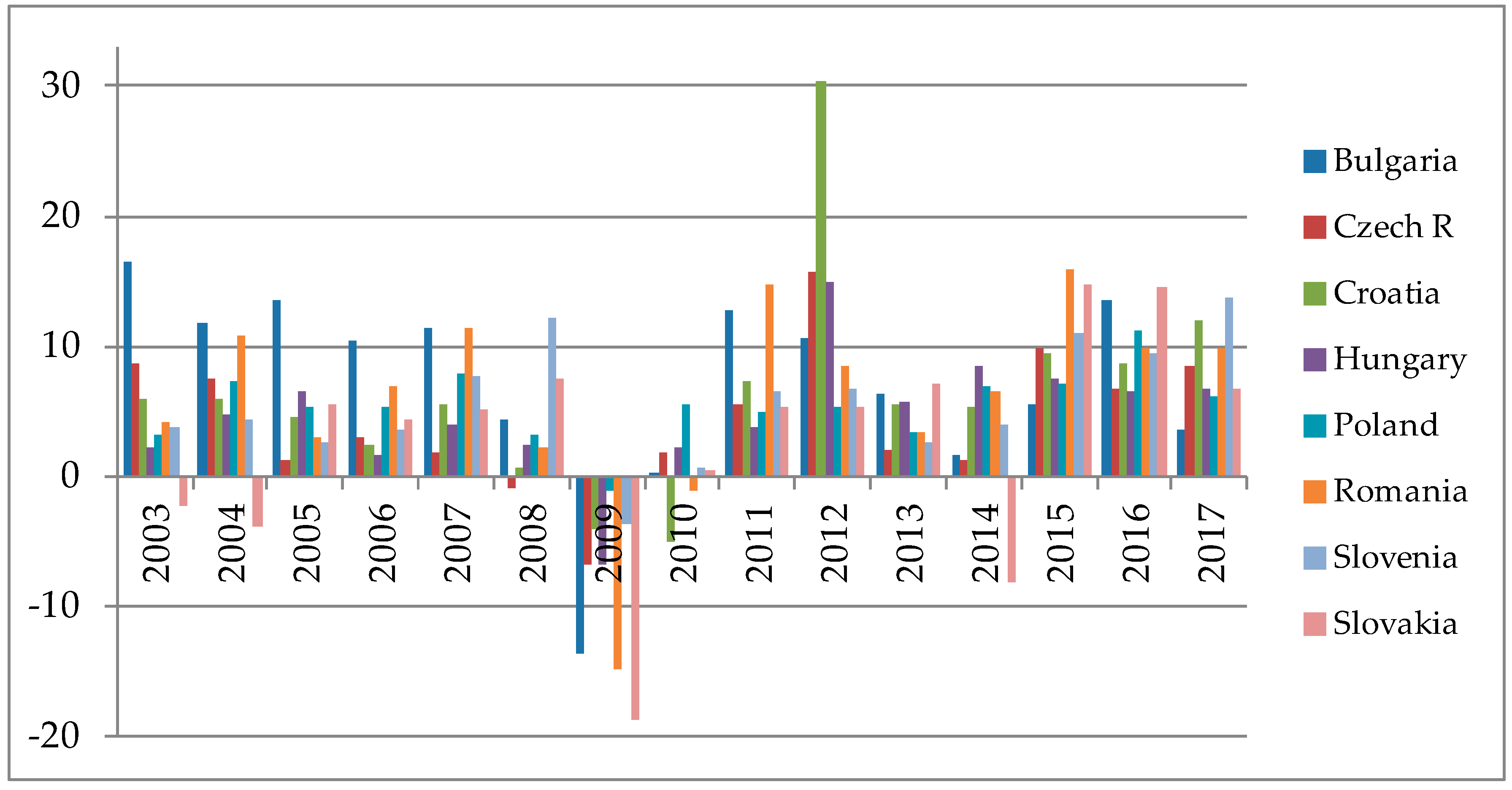
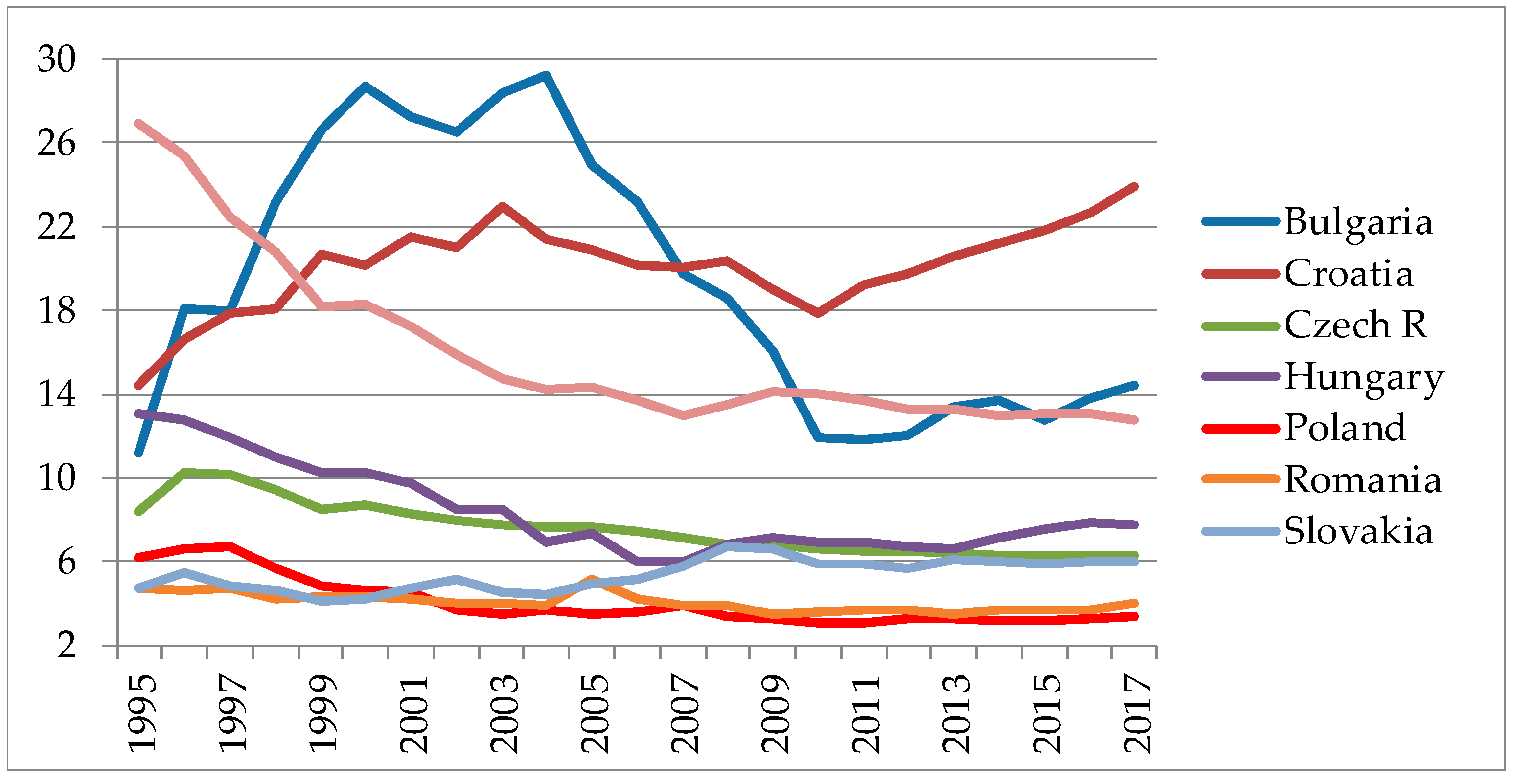
Overall yearly growth rates of total tourist arrivals for every country in the analysis are depicted on
Figure 1. It can be seen that there is a somewhat similar pattern of behavior (e.g., changes due to the financial crisis and the recovery afterwards). However, these countries have different types of tourism which they offer, thus the impacts of tourism to the overall economy and vice versa could be in place. For example, whilst Slovenia mostly offers winter tourism, Croatia mostly focuses on summer tourism and some countries do not have access to the sea (e.g., Slovakia). Other relevant indicators of tourism contributions to the economy are shown in
Figure A1,
Figure A2,
Figure A3 and
Figure A4 in the
Appendix.
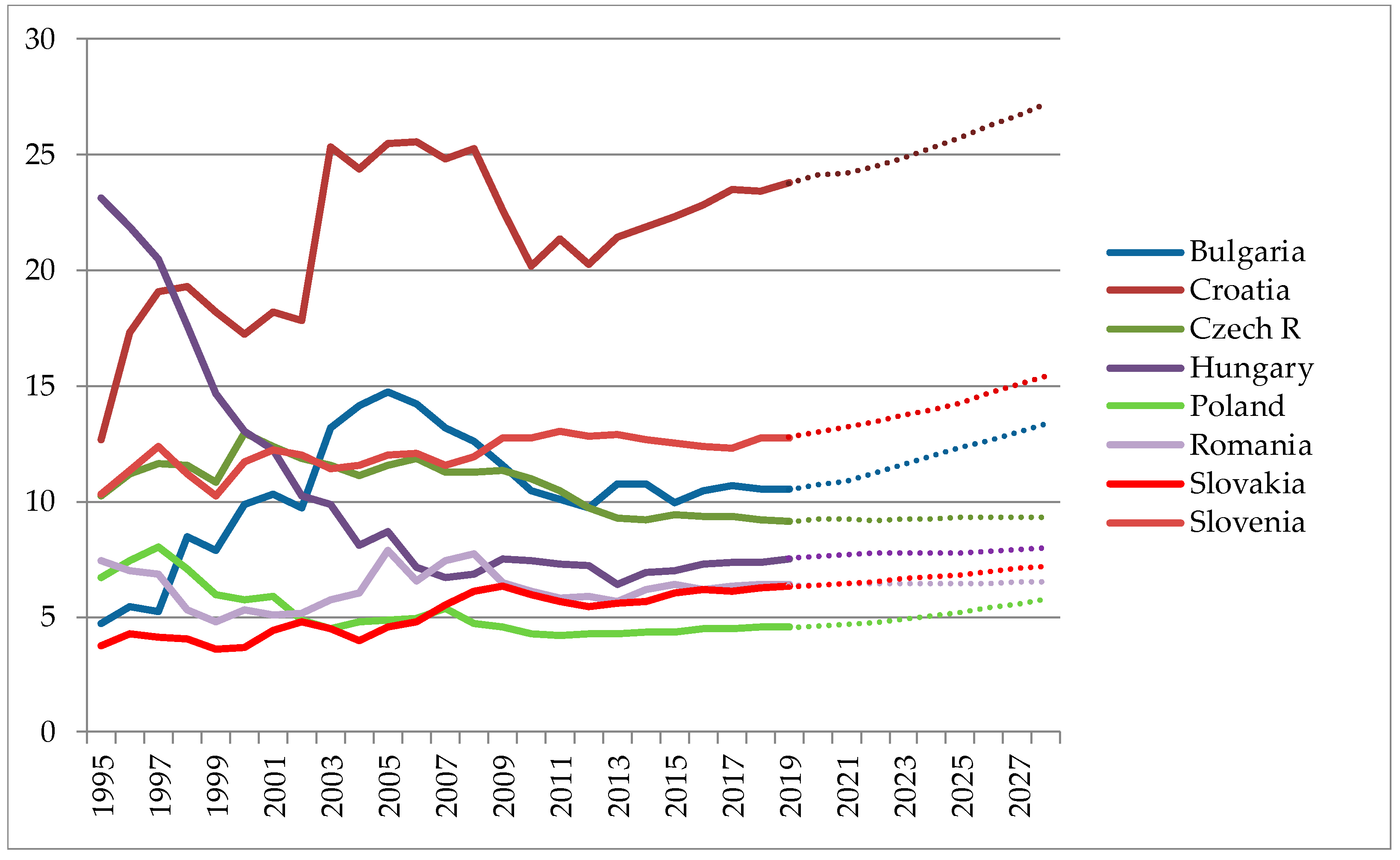
Figure A1 depicts the percentage share of tourism employment in the total employment, with forecasted values for the future. The crisis of 2008 has, of course, negatively impacted all of the countries; however, Croatia is showing greatest results (due to the coastal and summer tourism which is extending in the last couple of years and the demand for tourism related labor is increasing). Poland and Slovakia show a rather slow growth, with a very small percentage of tourism in total employment. Very similar conclusions are in place in
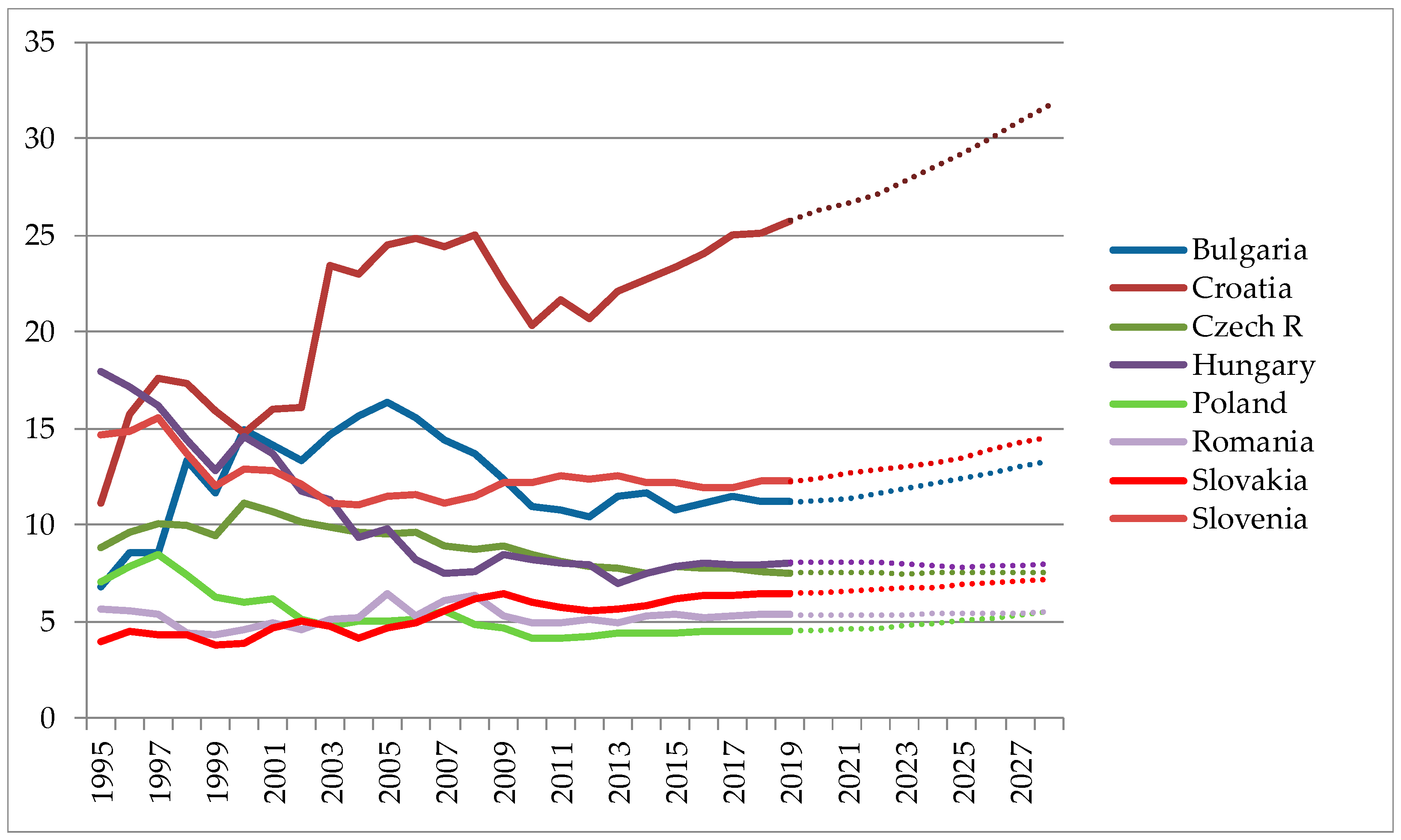
Figure A2, where the percentage share of total tourism contribution to GDP is shown. The growth for some countries is forecasted to be slow, which could be corrected if timely decisions are made. Thus, it is of importance to know the dynamic relationship of tourism demand and economy growth.
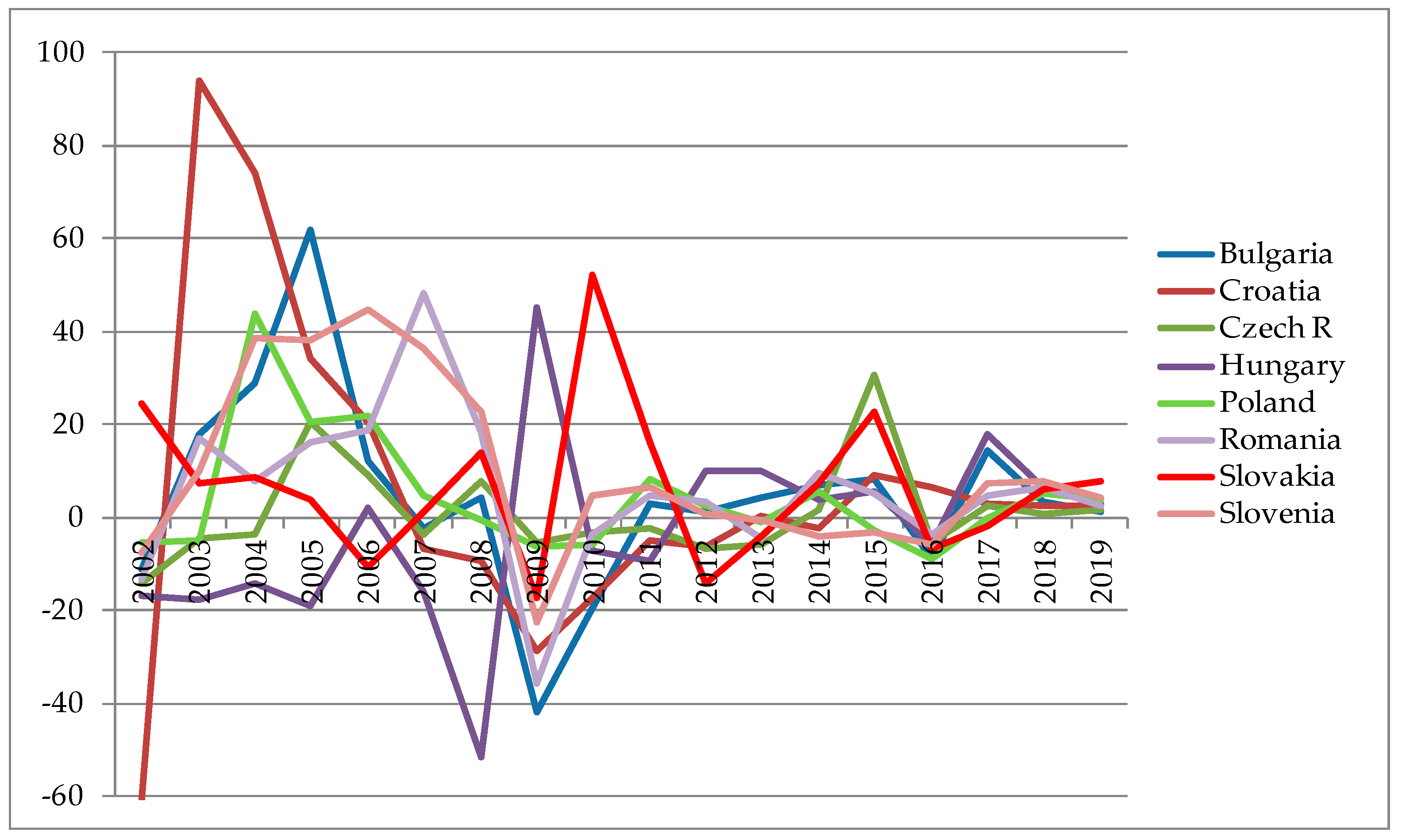
Figure A3 focused on percentage growth of capital investments into the tourism industry, in order to obtain some initial insights into the feedback from the real economy side to the tourism industry. All of the countries experienced volatile growth of capital investments during the observed period. This could be an indicator that formal policies were not focused enough on long term plans in order to develop the tourism infrastructure needed for a quality tourism development. E.g., Croatia experienced a lack of planning of infrastructure construction after the war of independence (see
Škrinjarić 2018). The positive side is that all of the countries experienced positive growth rates of capital investments into tourism industry in the last two years. This means that tourism demand is increasing in a way that new investments are needed in order to fulfill it. Finally, before the formal analysis, a brief description of
Figure A4 (percentage share of total tourism spending in GDP) tells us the following. Here, the differences matter in terms of if they exist due to great tourism spending in some country, or due to having bigger economies (e.g., Poland) in which the GDP is so great that tourism spending has a small percentage in it, compared to the smaller economies (e.g., Croatian economy).
Since time spans for all of the countries vary in the analysis due to the (un)availability of data, details on the available time spans are given in
Table A1 in
Appendix. Firstly, the original series were seasonally adjusted via multiplicative method and the month on month growth rates have been calculated by using the continuous return rates. Unit root tests (Augmented Dickey-Fuller) have been performed on the growth rates of tourism (TUR) and index of industrial production (IIP) with details in
Table A2 in the
Appendix. Since all of the variables were found to be stationary, they are suitable for the VAR model. The optimal length for each VAR model was chosen based upon the information criteria. Details are given in
Table A3 (see
Appendix). Based upon every VAR model for individual countries, the total spillover index was calculated based upon the 12 month ahead (
h = 12) forecast error decomposition and with the GFEVD decomposition of the variance-covariance matrix of innovation terms.
The spillover tables are provided in
Table 2,
Table 3,
Table 4,
Table 5,
Table 6,
Table 7,
Table 8 and
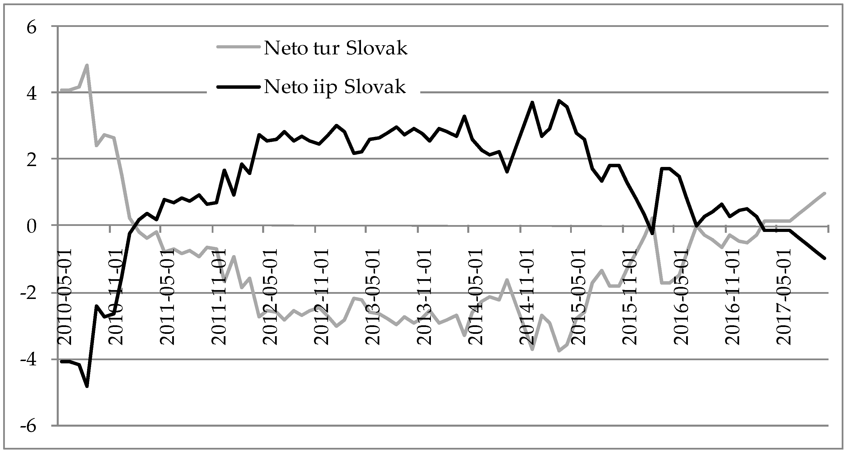
Table 9, with the total spillover index bolded in the left bottom right corner. The results are interpreted as follows, e.g., Bulgarian data is in the first table and the values in the first row are read as shocks in the TUR explain 89.15% of the forecast error variance of the same variable and 20.85% of IIP. The total spillover index is equal to 3.21%. Similar interpretations can be made for all other countries in the sample. The greatest spillovers between the tourism growth and the IIP growth were found for Slovenia, Hungary and Slovakia, meaning that greatest interaction between these two variables were found for those three countries. Next, by comparing indices “from” and “to”, information could be obtained on whether a country has tourism-led growth or growth-led tourism. In that way, tourism-led growth is found only for Poland, whilst other countries have growth-led tourism in the observed period. This is due to the greater values of “from” spillover indices for IIP compared to TUR, with exception for Poland. On average, the total spillover index was the greatest for Slovenia and smallest for Romania, meaning that the greatest interaction between tourism and economic growth was for Slovenia, whilst smallest for Romania.
Since
Table 2,
Table 3,
Table 4,
Table 5,
Table 6,
Table 7,
Table 8 and
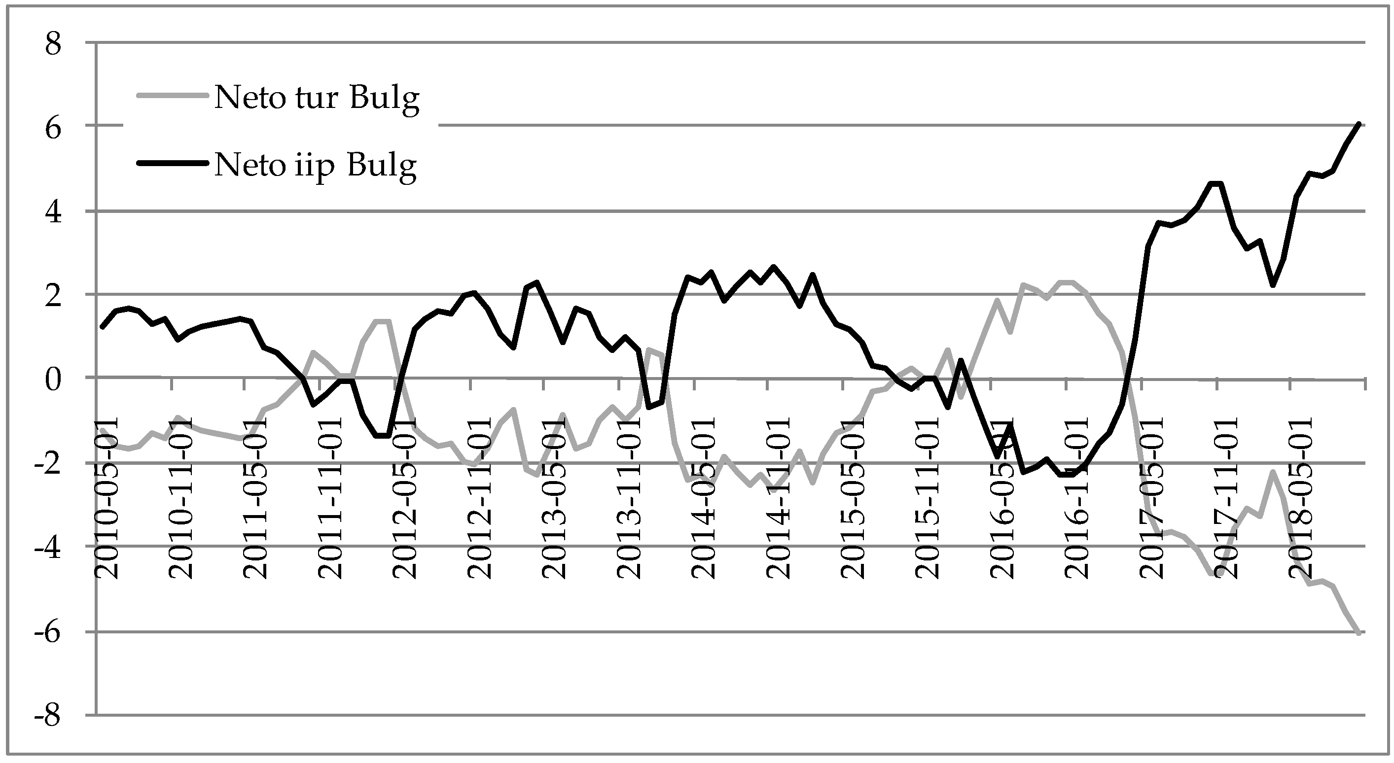
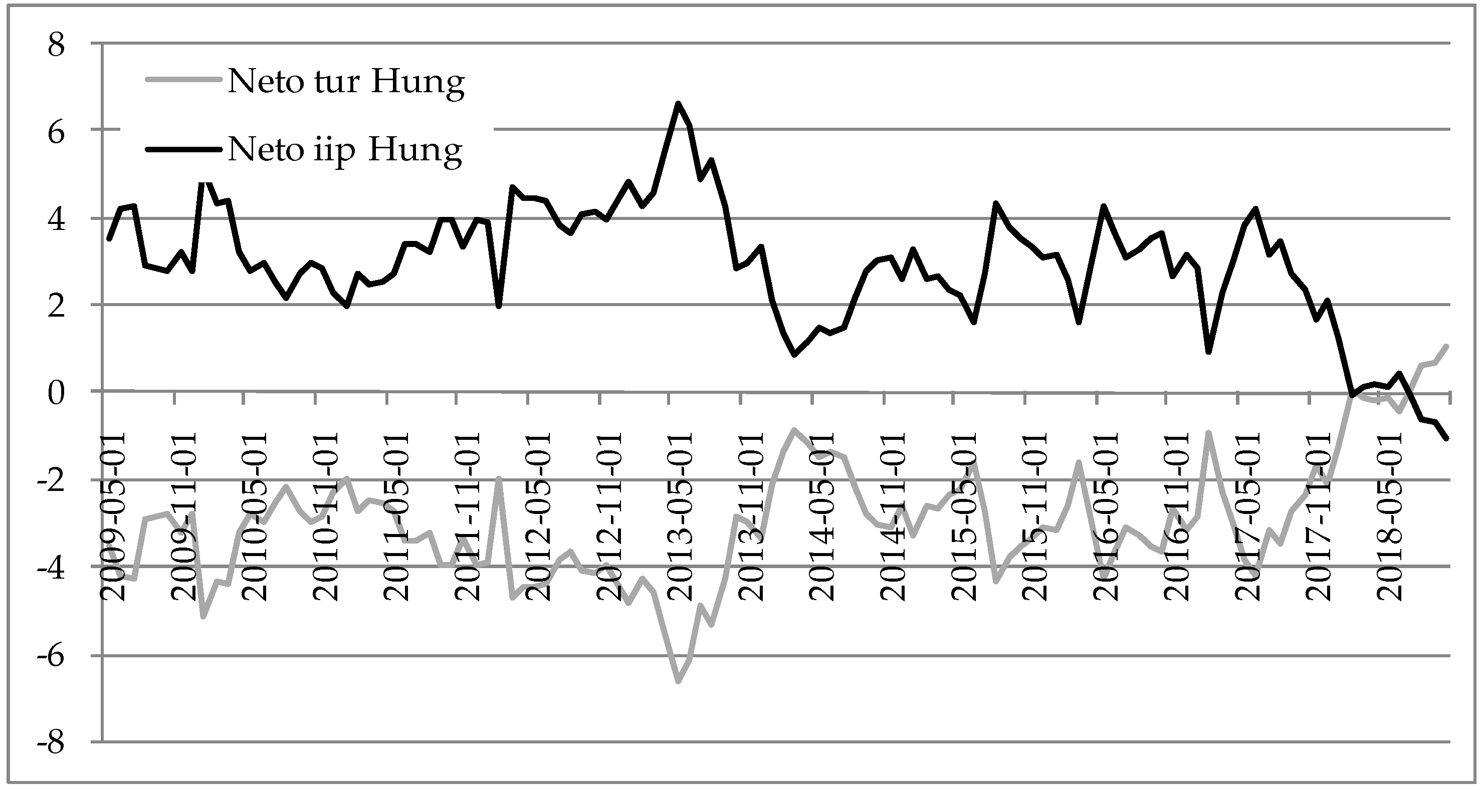
Table 9 give an overall average for the whole observed period, dynamic, i.e., rolling indices were estimated for every country and were depicted on
Figure 2,
Figure 3,
Figure 4,
Figure 5,
Figure 6,
Figure 7,
Figure 8 and
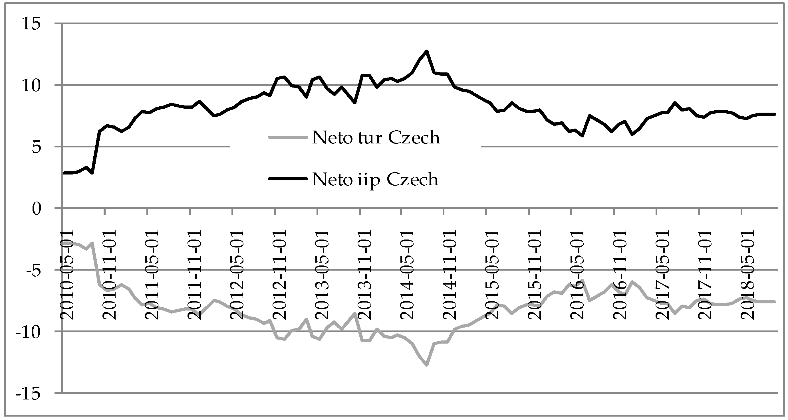
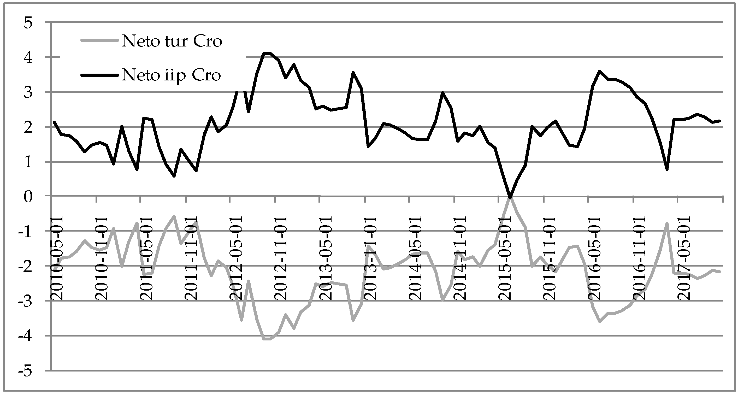
Figure 9. Based upon the “from” and “to” indices, the net indices were constructed for IIP and TUR. All of the countries with exception of Poland show that they experienced growth-led tourism in the majority of the examined period. If the value of the net index is positive, this means that this variable was the shock source (transmitter) rather than receiver. Bulgaria experienced strict spillovers from IIP to TUR in the last two years, which could indicate that this country is achieving good strategic planning of tourism development. Before these reversals, tourism-led growth was in place, as in
Aslan (
2013). Czech Republic had constant positive net index for IIP in the whole period, as well as Croatia. Growth-led tourism for Czech Republic is confirmed as in previous research of
Chou (
2013)
21 in which Granger causality was applied (as in other papers mentioned here which are used for comparisons
22). The results for Croatia are in line with
Payne and Mervar (
2010), in which the long-run causality tests resulted in favor of the growth-led tourism hypothesis; and
Hajdinjak (
2014), in which the Granger test implied that tourism should not be considered as a key sector of the economy growth, with the reasoning being that the contributions of the tourism sector to the whole economy was being overemphasized over the years.
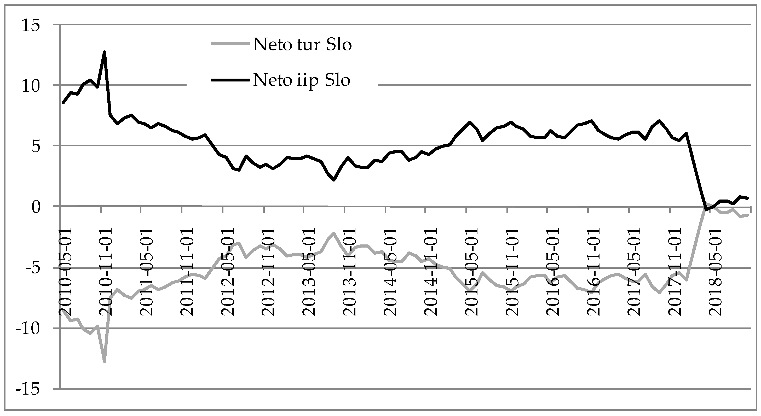
Hungary and Slovenia had positive net index for IIP until the end of the period. The results for Slovenia are in line as results of growth-driven tourism in
Gričar et al. (
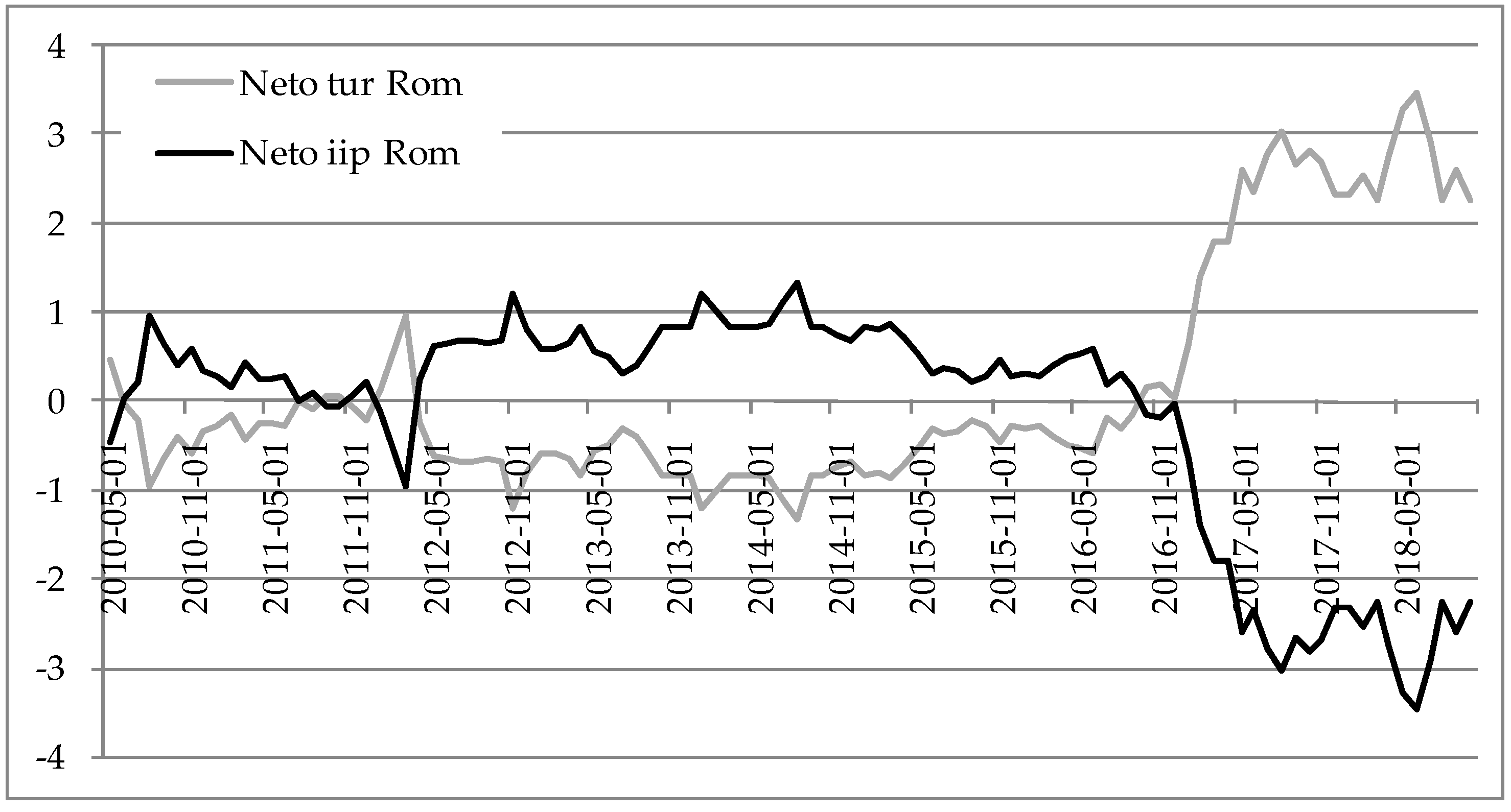
2016). Romania experienced a reversal in 2017 and 2018 between two net indices (TUR became net exporter of shocks) and this is due to the increase of tourist spending in those two years, surpassing 8% of total GDP for the first time since the financial crisis. In previous years, this country experienced mostly growth-led tourism, which is in accordance in
Oh (
2005) who states that, in countries with small contributions of tourism industry to the GDP, there is a greater probability that the economy will be characterized with the GLT hypothesis. The mixed results for Bulgaria and Romania are in line with
Chou (
2013), in which both directions from tourism to economic growth and economy-led tourism growth are found. This is due to interweaving of net indices for both countries. Slovakia experienced a significant change in net indices from 2010 to 2011 due to enormous change in capital investment in the tourism industry in 2010 (more than 50% increase,
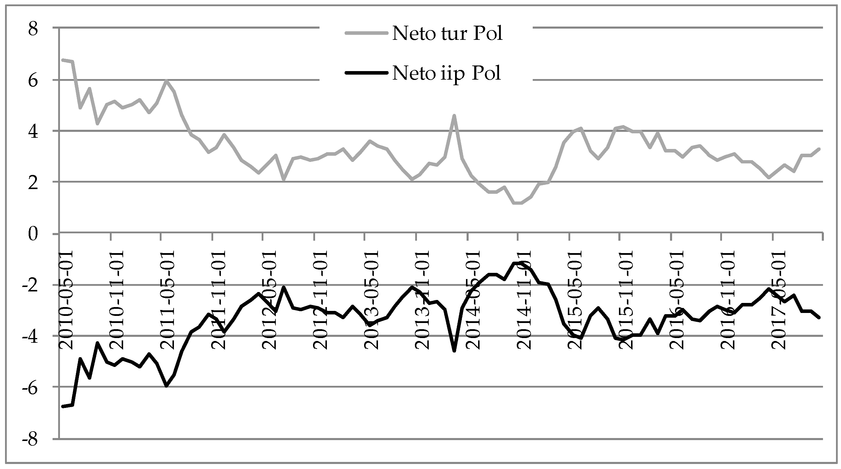
WTTC 2019). This was reflected in later years with Slovakia having a positive net index for IIP compared to the net receiver TUR. Poland experienced tourism-led growth in the whole period.
Table 10 depicts summary results for the rolling indices on
Figure 2,
Figure 3,
Figure 4,
Figure 5,
Figure 6,
Figure 7,
Figure 8 and
Figure 9. Countries were divided solely on the criterion of positive or negative net TUR spillover indices. Differences between the minimal and maximal values for every rolling index are visible on the mentioned figures as well.
Based upon the results, several recommendations can be provided for policy makers in the observed countries. Although there is a lot of related research with different methodologies applied, the dynamic approach in this paper enables re-evaluation of current policies. This means that although economic measures and plans can be brought for a longer period of time, they can be evaluated via the methodology used in this research; and, if needed, those plans could be tweaked and modified accordingly. Since forecasts are often difficult to make, especially longer into the future, re-evaluation of the spillovers between tourism growth and economic growth could provide guidance for achieving better results. Majority of countries observed in this research are not as developed as some other countries in Europe. This means that these countries could utilize tourism industry to achieve a faster economic growth, as
De Vita and Kyaw (
2016) explain that more developed countries have diminishing returns to scale on tourism effects on the economic growth. This could potentially be true for the countries for which this study found the TLG hypothesis to hold in the majority of the observed period (Poland). Each individual country in this sample surely knows its weaknesses and strengths regarding tourism supply and industry as a whole. Since the results in this research indicate mixing within the sample (some countries had GLT over the whole sample, others the opposite direction of spillovers), policy makers should focus on individual characteristics of every country in order to examine why some reversals of spillovers were found on
Figure 2,
Figure 3,
Figure 4,
Figure 5,
Figure 6,
Figure 7,
Figure 8 and
Figure 9. In that way, future decisions could be tailored more specifically to the advantages and disadvantages of the specific country. This is in line with previous panel data research, in which authors find heterogeneity in results (see
Chou 2013). The methodology in this study focuses on individual countries and this could be considered as an advantage compared to panel data studies with heterogeneous data and results.
5. Conclusions
Although the tourism-led growth and growth-led tourism hypotheses are discussed in the literature for many years now, the empirical research sometimes provides contradictory results for the same country. This is mostly true for studies which use the static approach of estimating the relationship between tourism and the economy, which contributes to this problem, alongside using different variables and time spans in the research. This study opted to obtain the longest time span possible for every country in the analysis and to estimate a dynamic spillover index between tourism and economic growth. In that way, if the relationship is changing over time. this could give researchers and practitioners more correct information. The overall results implicate that Poland should utilize the tourism led growth results before reaching greater development, as this would bring rising return performance for the GDP growth at this point. Czech Republic, Hungary, Slovenia and Croatia should focus more on achieving greater overall economic development so the spillovers to the tourism industry could be even greater. This is especially true for Croatia, in which due to migrations of the labor force to the rest of the Europe, the economy will face problems in the long run. It seems that Romania is on a right path for promoting tourism led growth in the last two years. Thus, it should focus now on the tourism content which is being demanded. Bulgaria had bi-directional spillovers for both variables, which could mean that this country found a good balance between investing into tourism development which spills over to the economy and vice versa. Finally, Slovakia already carried out some changes in early 2010s, when major capital investments were done regarding tourism industry and now should continue to focus on spillovers from the rest of the economy to the quality of tourism industry.
The shortcomings of the paper were the following ones. Firstly, we observed only 8 CEE/SEE countries, due to data unavailability. Moreover, since part of the total time span has to be used to estimate the VAR model with sufficient data in order to obtain reliable results, the pre-crisis and crisis period could not be included in the estimation of rolling spillover indices. It would be interesting to observe which countries were more successful to bounce back to pre-crisis trends. Thus, positive practices could be observed. Moreover, the total time span is also relatively short compared to other studies in which more developed countries are in focus. This is why often CEE/SEE countries are left out from analyses. The same is true regarding the topic of this paper (as it was seen in literature overview). Moreover, only two variables were observed with the spillover methodology (due to estimating total effects between them). Further research should extend not only the time span used in the analysis, but it should try to observe interaction between other tourism demand variables. This research followed previous literature and we opted to use the most common variable (tourist arrivals). Since some data exists on domestic and foreign tourist arrivals, this could be another direction for future research.
However, some of the results obtained in this study also provide at least some help in determining on the changing relationship between tourism and economic growth. In this way, policy makers and others involved into the tourism-economy relationship on every level of the economy can focus more on those time spans in which some meaningful changes in the spillover indices were in place. Relevant agents can focus on what specifically was happening in the economy, tourism demand and supply when some specific changes occurred. To conclude, many opened questions are left for future work for researchers in individual countries observed in this study regarding enhancing the results from the relationship between tourism and economic growth.


