1. Introduction
Substantial attention has been paid to the examination of economic growth—public debt nexus. In theory we can find arguments for positive, negative or neutral effect of government borrowing on economy. From Keynesian point of view, expansionary fiscal policy leads to higher debt level and simultaneously stimulates GDP growth, especially through the mechanism of expenditure multiplier. However, this positive effect is expected mostly in the short-run. The neo-classical theory asserts harmful impact of public debt, known as crowding-out effect. Government borrowing can result in higher interest rates and thus reduce private investment and growth. Ricardian equivalence suggests that public deficit and debt do not make influence on growth. Increase in demand because of debt-financed government consumption is offset by rising savings. People save more as they prepare for future tax increase, when it will be necessary to repay high public debt.
In the sample of 20 developed countries,
Reinhart and Rogoff (
2010) find negative relationship between debt and economic growth, when public debt to GDP ratio exceeds 90 percent.
Pattillo et al. (
2011) estimate much lower threshold for the panel of 93 developing countries. The debt levels above 30–40% of the GDP start hindering per capita growth.
Checherita-Westphal et al. (
2014) conclude that optimal debt to the GDP ratio for Euro area is around 50% and 65% is for the sample of 22 OECD countries.
A. Baum et al. (
2013) perform regression analyses for 12 Euro zone countries and indicate that the negative debt-growth relationship occurs when the debt level exceeds 95% of the GDP. To avoid reverse causality
Woo and Kumar (
2015) examine the impact of initial debt level on subsequent growth (5–20 years) of real GDP per capita in a panel of 38 advanced and emerging economies. They found some evidence for the threshold of initial debt-to-GDP ratio of 90%, having larger negative effect on the growth in the future.
Afonso and Jales (
2013),
Herndon et al. (
2014) obtain the opposite results. They found no evidence that the GDP growth of the countries with high levels of debt (above 90% to GDP) is different from ones with low debt ratios. The results obtained by
Panizza and Presbitero (
2013),
Egert (
2015) are in line with this conclusion. The authors conclude that the presence of the threshold above which government debt starts having detrimental effect on growth is not robust and sensitive to the analysis period, country coverage and other modelling choices.
The estimated threshold value above which the impact of debt on growth becomes harmful varies between 30–95% of GDP and gives a little insight into what the optimal level of debt is. As
Panizza and Presbitero (
2013) point out, it might be impossible to find a single debt tipping point that holds for all countries, because a range of factors can shape the impact of debt on growth. In recent research on debt-growth nexus,
Kim et al. (
2017) highlight, that despite a huge amount of empirical work that has been done to investigate the relationship between public debt and economic growth, not much attention has been dedicated to an important explanatory factor—institutional quality. Most of empirical research employ panel data models assuming, that the debt impact on growth is common for all observations. However, this relationship could be influenced by country-specific factors of which quality of institutions is one of the most important. Only few studies investigate whether the countries’ ability to deal with negative borrowing effect depends on the institutional factors. Authors employ the aggregate measure of institutions or focus on specific aspects, such as democracy or corruption.
Presbitero (
2008,
2012),
Cordella et al. (
2010),
Megersa and Cassimon (
2015) use Country Policy and Institutional Assessment (CPIA) index, which covers various characteristics of public sector management quality: transparency, property rights, quality of financial and budgetary management and so forth.
Masuch et al. (
2016) employ the aggregate measure of four Worldwide Governance Indicators, namely government effectiveness, regulatory quality, rule of law and control of corruption.
Jalles (
2011),
Kourtellos et al. (
2013) investigate how the debt-growth interaction depends on the level of democracy or corruption.
Matemilola et al. (
2016) focus on legal origin and compare the results obtained in the samples of civil and common law countries. It is worth mentioning that there is still no agreement in scientific literature whether the above mentioned indices measure institutions or their outcomes.
Voigt (
2013) presents a more detailed discussion on this issue.
Most of the results suggest that sound institutions can help to deal with detrimental debt impact on growth. Countries with a better institutional quality can borrow more without facing a slowdown effect on economy. However,
Presbitero (
2008,
2012) concludes the opposite: debt constrains economic growth only in countries with strong institutions, while in countries with bad policies and weak institutions this effect is irrelevant.
The institutional quality is shown to be a crucial factor which has an influence on the relationship between economic growth and public debt. The literature on other possible sources of heterogeneity is rather scarce.
Kourtellos et al. (
2013) test a large set of probable variables which might explain the heterogeneous influence of debt on economic growth but find the strongest support for the threshold effects based on the quality of institutions proxied by democracy index.
Marchionne and Parekh (
2015) conclude that debt threshold level depends on the level of income inequality. The state of financial market (
Proano et al. 2014), country risk (
Chiu and Lee 2017) and economic systems (
Ahlborn and Schweickert 2018) are found to be a source of debt—growth relationship heterogeneity. This paper seeks to supplement empirical evidence on the factors, which shape debt impact on economic growth and aims to investigate whether debt threshold level depends on government effectiveness (one of the aspects of countries’ institutional quality) and trade balance. Notwithstanding a vast literature on the relationship between fiscal deficit and trade deficit, as far as we know, there is a lack of empirical evidence on possible trade balance effect on the debt tipping point above which government borrowing impedes economy. The theory suggests that ability to stimulate growth by borrowing funds for public expenditure depends on the value of fiscal multiplier, which tends to be low (or even negative) if countries are relatively open (
Silva et al. 2013;
Ilzetzki et al. 2013;
Batini et al. 2014). Relying on this, we raise the hypothesis that countries with higher government effectiveness and lower level of trade deficit have higher debt threshold (turning point) level. We can find some empirical evidence that countries with better institutional quality (proxied by indices representing government effectiveness, corruption, democracy, etc.) can borrow more before facing debt slowdown effect on economic growth. In addition to this, in this paper we argue that countries where the institutional quality (measured by government effectiveness index) is relatively similar might have different debt threshold (turning point) levels if we take the level of trade deficit into account. Both factors, that is, government effectiveness and trade deficit, are shown to be possible sources of debt impact on economic growth heterogeneity.
The rest of the paper is organized as follows: the second and the third sections of this paper describe the channels how institutional quality (
Section 2) and trade balance (
Section 3) might influence the public debt—growth relationship.
Section 4 presents the data and the model.
Section 5 discusses general estimation and
Section 6—robustness check results.
Section 7 concludes the paper.
2. The Role of Institutional Quality in Debt-Growth Relationship
Debt can foster or hinder economic growth. While there is a huge amount of literature on this impact, only few recent studies focus on institutional aspects as a key factor determining debt influence on growth. The country can stimulate its economy by borrowed funds if they are used effectively and in moderation, while, used excessively and irresponsible, they will make a slowdown effect. There are diverse ways how institutional aspects may affect debt impact on growth. Empirical research provides evidence that governments in more corrupt countries borrow more as increase in corruption level is associated with increase in public debt (
Cooray et al. 2017;
Benfratello et al. 2018;
Njangang 2018). One may expect better fiscal sustainability performance in countries with good governance. Nevertheless, even efficient governments may be willing to fulfil the needs of their voters by financing consumption with debt (
Jalles 2011).
Institutions determine not only the level of debt but also the distribution of borrowed funds.
Shleifer and Vishny (
1993) argue that more corrupt governments tend to redirect loan resources from productive areas such as health and education to defend and infrastructure projects with lower value creation but better possibilities for corruption. Countries with common law system use public debt in a more efficient way compared with civil low countries (
Matemilola et al. 2016).
Melecky (
2012) points out that the good public debt management may reduce borrowing costs and restrict financial risks, however well-designed strategies more likely appear in countries with better institutional environment. Higher risk premium has to be paid when issuing bonds in corrupt (
Ciocchini et al. 2003) or politically unstable countries (
Baldacci et al. 2008).
Summing up, we can conclude that countries with weak institutions tend to borrow excessively, use loan resources irresponsible, redirecting them to less productive areas; the poor public-sector management quality results in higher borrowing costs. Due to the above mentioned reasons one might expect countries with sound institutions and good public-sector policies to be more successful in stimulating economy by increasing debt.
Most of the studies confirm the institutional aspects to be a crucial factor determining what influence debt will have on economic growth.
Kourtellos et al. (
2013) suggest detrimental debt impact to occur only under a particular level of democracy, while debt is neutral for growth in countries with good democratic institutions. The opposite findings are presented by
Presbitero (
2008,
2012) in the samples of developing countries. Debt is irrelevant to growth if country policies and institutions do not ensure favourable environment and have an adverse effect on economic development only when a country implements good macroeconomic policies and has sound institutions.
Dauda and
Podivinsky (
2014), analysing the data on Malaysia, indicate that whether debt fosters or hinders economic growth, depends on the institutional quality, measured by political rights, civil liberty and economic freedom indices. The positive effect occurs when institutional quality is high enough to ensure well-functioning government, which effectively distributes and allocates the borrowed funds to high value-added sectors. This conclusion to some extent is supported by
Megersa and Cassimon (
2015),
Masuch et al. (
2016),
Kim et al. (
2017) who include institutional quality and debt interaction variable into growth regression and find evidence that the negative effect of debt on growth is at least lower (if not turns to positive) when coupled with good policies and institutions.
Megersa and Cassimon’s (
2015) findings for 57 developing countries suggest that debt is detrimental for growth, however, harm is reduced while controlling the quality of public sector management.
Masuch et al. (
2016) results show that adverse effect of high initial debt levels (above 60%) on long term growth in the European countries might be offset by sound institutions, however the results are robust to changes in the measures of institutional quality.
Kim et al. (
2017) provide the comparable results in a sample of 77 advanced and developing countries focusing on corruption level as a measure of institutional quality. The growth is mostly restrained by growing debt in highly corrupt countries, whereas enhanced in transparent ones.
Cordella et al. (
2010),
Jalles (
2011),
Megersa and Cassimon (
2015),
Matemilola et al. (
2016) use alternative approach to test whether institutional quality might explain a different economic growth reaction to the debt level or its changes. The results are estimated and compared in the clusters of countries determined by various measures of institutions. To derive the debt threshold levels
Cordella et al. (
2010) split the sample of 79 developing countries into subsamples according to Country Policy and Institutional Assessment index, net private capital inflow and settler mortality (proxy for quality of institutions). The results confirm that debt threshold arises at different levels of debt, depending on conditions in the country. Besides this, another important insight is presented about the existence of second—debt irrelevance threshold, above which additional increase in debt has no effect on growth, that is, marginal effect is zero, while average one remains negative. The findings suggest that both debt threshold levels, first, when the marginal impact of debt and growth becomes negative and second, when it becomes zero, seem to be lower in countries with “bad conditions.”
Jalles (
2011) comes to a similar conclusion when divides 72 developing countries into sub-samples according to the control of corruption indicator. More corrupt countries start to have harmful impact on growth at lower debt levels.
Megersa and Cassimon’s (
2015) findings related to the estimates for the developing country clusters with “strong” and “weak” public sector management quality confirm that if public sector is poorly managed, government debt has a negative effect on economic growth but it turns into a positive effect in countries with “strong” public sector management quality.
Matemilola et al. (
2016) split 18 developing countries according to their legal origin into common law and civil law samples. The results indicate that the long-run economic growth is reduced by public debt in common law countries but effect is insignificant in the short-run. Conversely, public debt adversely affects the growth of civil law countries in the short-run, with no significant impact on the long-run growth.
The above mentioned studies confirm the institutional aspects to be a crucial factor determining what influence debt will have on economic growth, as sound public institutions ensure well-functioning government that manages public debt and distributes borrowed funds in the most efficient way. This supports our assumption that countries with more effective government can have higher debt to GDP ratios without detrimental effect on economic growth.
3. The Relationship between Trade Balance and Government Debt
The idea of this paper is related to the assumption that the level of government debt threshold depends on the country’s trade balance. Despite the lack of empirical evidence on this relationship, there is a lot of empirical studies on the interdependence of budget balance and trade balance. Governments borrow to finance budget deficit and thus increase country’s debt, so the relation of budget balance and trade balance can also be considered as a link between debt and trade balance. The Keynesian “twin deficit hypothesis” suggests a close connection between budget deficit and trade deficit. This connection can be explained by using the macroeconomic leakages-injections model which is used to identify the equilibrium level of income:
where S—savings, T—taxes, M—imports, I—gross private domestic investment expenditures, G—government expenditures, X—exports.
Reorganizing the equation, we get:
The trade balance (X − M) depends on the private (S − I) and public (T − G) savings. This equation is a core of “twin deficits” hypothesis. Budget deficit refers to increased public spending, which results in expanded aggregate demand for both domestic and imported goods. The import growth leads to the deterioration of trade balance. Keynesian theory implies “crowding out” effect, that is, government borrowing reduces funds available for private investment and results in increased interest rate. Higher domestic interest rate is favourable for international fund inflow, which raises the exchange rate of domestic currency and thus detracts exports, enhances imports, so trade balance is worsened.
A number of empirical studies support “twin deficit” hypothesis and also conclude that causality runs from the budget deficit to trade deficit (e.g.,
Hye and Ali 2010;
Tang 2015). Other studies agree on the trade and budget deficit relationship, nonetheless, they provide the alternative explanation of causality. Trade deficit leads to a lower economic growth, which in turn might result in a higher budget deficit. Empirical support for this link can be found in a number of studies, however most of them employ current account balance variable instead of trade balance (for the most recent results and the survey of earlier studies, see
Senadza and Aloryito (
2016);
Amaghionyeodiwe and Akinyemi (
2016);
Helmy (
2018)).
Some studies provide mixed evidence, where the results support causality from budget deficit to current account deficit in some countries and opposite causality in other ones (
Carrasco 2016;
Ravinthirakumaran et al. 2016) or confirm the bidirectional causality (
Bolat et al. 2014;
Xie and Chen 2014). However, researchers question the causal relationship between budget and trade deficits. Their arguments rely on the Ricardian equivalence hypothesis. When budget deficit increases, households start preparing for future tax increase and save more, thus, according to Equation (2), increase in private savings (S − I) offsets decrease in public savings (T − G) with no impact on trade balance.
Amaghionyeodiwe and Akinyemi (
2016) provide more detailed arguments and the review of empirical support for this hypothesis.
Another theoretical background for our assumption is related to the fiscal multiplier effect. When the government is borrowing to finance its expenditure, the aggregate demand and economic growth can be expected to increase. However, this effect depends on the size of multiplier effect. A detailed review on factors shaping value of fiscal multiplier and its estimation techniques can be found in
Boussard et al. (
2013),
Silva et al. (
2013),
Batini et al. (
2014). The value of a fiscal multiplier (or most of its determinants) is unknown at a particular time and it makes difficult to assess what impact government expenditure will have on economic growth. This fact notwithstanding one can rely on certain available data—trade balance. The higher the marginal propensity to import, the lower the value of fiscal multiplier, as imports are a withdrawal of demand (
Batini et al. 2014).
Summing up, one might expect that increase in budget deficit stimulates aggregate demand for domestic and imported goods. If latter impact dominates and the value of fiscal multiplier is low (or negative), borrowing to finance excess government spending results in growing debt level with no or even negative impact on economic growth. This supports our assumption that trade balance can be a key factor shaping public debt impact on economic growth.
4. Data and the Model
The data used in this research is an unbalanced panel of 152 countries over the period of 1996–2016. We measured 5-year average growth rate of per capita gross domestic product (GDP) with the log difference per capita GDP in constant 2010 U.S. dollars from the World Development Indicators (WDI) database of the World Bank (WB). Gross fixed capital formation (GFCF), Consumer price index (CPI), Population (POP), Import (IMP), Export (EXP), General government final consumption expenditure (G), Secondary school life expectancy are also from WDI and Government effectiveness (GE)
1 is from WB’s Worldwide Governance Indicators (WGI) database. General government gross debt (GGGD) in terms of GDP is from the World Economic Outlook (WEO) database of the International Monetary Fund (IMF). The summary statistics of variables and their description are presented in
Table A1 (see
Appendix A).
Following the survey of the literature on the public debt-growth relationship (
Panizza and Presbitero 2013) most studies use a standard growth regression model, where as a set of controls (besides government debt) includes the standard Solow model variables: population growth, investment and human capital measures.
Following the standard neoclassical growth model, first, we controlled the initial real GDP per capita, since this growth model emphasizes convergence hypothesis. The second controlled variable is investment to GDP ratio, representing the rate of factor inputs in the production function. In consistency with the basic and augmented Solow model (
Mankiw et al. 1992) and based on the empirical findings by
Levine and Renelt (
1992), we included the growth rate of population (log[POP
t] − log[POP
t−1]) and secondary education (as a proxy for human capital we used the logarithm of secondary school life expectancy in the initial year of each period) was taken as a measure of investment in human capital. Initial change in prices, as suggested by
Megersa and Cassimon (
2015),
Kim et al. (
2017), is controlled as well—we used inflation rate (log[CPI
t] − log[CPI
t−1]) in the first year of each period. The openness (exports plus imports in percent of GDP) and government size (government expenditure as a share in GDP) variables represent country-specific policy and are typically included in panel regression equations, examining differences of long-term growth across countries (
Masuch et al. 2016).
Following recent studies (e.g.,
Marchionne and Parekh 2015;
Matemilola et al. 2016;
Ahlborn and Schweickert 2018), we estimated non-linear impact of debt on economic growth. The arguments, why negative debt impact on growth is more likely to occur with higher debt levels, are related to debt effect on capital accumulation, future taxation and inflation (
Ramos-Herrera and Sosvilla-Rivero 2017).
Referring to Piketty (
2015),
Arrow (
2017) and
Fingleton (
2017), we also included the squared investment term to capture the possible non-linear relationship and diminishing marginal growth effect of investment. The basic dynamic panel data model is expressed as follows:
where
i and
t stand for a country included in the analysis and the time period, respectively.
gdpi,t+5 is the real per capita GDP of a country
i five years ahead. The initial per capita GDP and other variables up to
debt of a country
i at the beginning of the period are presented in
Table A1. The remaining variables
μt and
λi are time-specific fixed effect and country-specific time-invariant effect, respectively. The last term
εi,t, is the time-varying error term.
Given that economic growth is measured as log-difference of per capita real GDP (log[
gdpi,t+5]-log[
gdpi,t]), Equation (4) that could be used to examine debt–growth relationship is equivalent
2 to the dynamic panel data model:
where
gri,t→t+5 the average growth rate of the real per capita GDP of a country
i over five years. Following the vast majority of cross-country empirical studies, we used overlapping five-year periods (1996–2001, 1997–2002 and so on up to 2011–2016) to calculate average growth rate.
Panizza and Presbitero (
2013) conclude that the interval of 5 years is usually used in the research to mitigate the problem that the estimates based on annual data are dependent on the business cycle fluctuations and suffer from endogeneity. (
β0 − 1) is the convergence coefficient and
X is the set of standard control variables as in Equation (3).
Aimplied in Equations (3) and (4), the marginal effect of public debt on economic growth is calculated as follows:
If we assume a quadratic form of debt–grow relationship, Equation (5) shows that the marginal effect of public debt on economic growth might depend on public debt amount. Put in other words, the marginal effect is not constant across countries but is conditioned upon how indebted a specific country is. Referring to recent studies on the public debt-growth link (e.g.,
Marchionne and Parekh 2015;
Matemilola et al. 2016;
Ahlborn and Schweickert 2018), we expect that estimated coefficients on
β8 and
β9 will be positive and negative, respectively, implying that exceeding a certain public debt level, the public debt-growth relationship becomes negative. We also think that the marginal effect of public debt on growth and turning point in the direction of public debt-growth relationship is not universal and conditioned upon institutional quality as well as on trade deficit as it was discussed in
Section 2 and
Section 3.
As it was discussed in
Section 2, to examine the heterogeneity of public debt-growth relationship, the studies include institutional qualities and public debt interaction variable into growth regression or split the sample of countries according to the quality of institutions. In this article we employed both strategies. First, we split our sample of 152 countries into 4 subsamples according to trade balance and government effectiveness indicators. Second, for the robustness check, we included public debt and government effectiveness, public debt and trade deficit ieraction variables. The median level of import-export ratio in total sample (i.e., 1.2) is used as a threshold to assign a country (according to time-average ratio) to a group of relatively high (IMP/EXP ≥ 1.2) or relatively low or no (IMP/EXP < 1.2) trade deficit countries. Country is assigned to a group of territories with relatively low government effectiveness if the time-average of government effectiveness indicator is below 0 and otherwise to a group of territories with relatively high government effectiveness. The distribution of countries is provided in
Table A2 and the descriptive statistics of variables in separate subsamples are provided in
Table A1. To explore whether public debt-growth relationship depends on trade deficit and quality of government effectiveness, we will estimate Equation (4) with pooled (cross-country, time series) datasets consisting of 12 countries characterised by relatively high trade deficit and high government effectiveness, 55 countries that have low government effectiveness and relatively high trade deficit, 52 countries with high government effectiveness and low or no trade deficit and finally 33 countries characterised by small or no trade deficit and low government effectiveness separately (see
Table A2 in
Appendix A).
Equation (4) being in a dynamic structure leads to upwards biased and inconsistent OLS estimator, because initial level per capita GDP correlates with the error term. The within transformation would not help either, since LSDV estimator, as
Nickell (
1981) emphasized, will be downward bias and inconsistent in the dynamic structure. A possible solution is proposed by the Generalized Method of Moments (GMM) technique. However, as
Blundell and Bond (
1998) argue, when
β0 is close to one, so that the response variable follows a path similar to a random walk, the GMM proposed by
Arellano and Bond (
1991) is downward bias and has the poor finite sample properties, in particular dealing with the small number of periods. Nevertheless, GMM estimator could be to some extent used to analyse growth factors. Referring to recent contributions to growth literature, we will count on a system-generalized method of moments (SYS-GMM) estimator proposed by
Arellano and Bover (
1995) and
Blundell and Bond (
1998) to examine the impact of public debt (
debti,t) on economic growth (
gri,t→t+5) in Equation (4). The SYS-GMM estimator is derived by simultaneously estimating two equations, one in levels (that uses lags of once-differenced regressors as instruments) and another in first differences (that uses lagged levels of regressors as instruments). As
Blundell et al. (
2001) argue, in a multivariate dynamic panel context SYS-GMM estimator outperforms GMM estimator when series are persistent (that is
β0 close to one) and exploiting additional moment conditions leads to a reduction in the finite sample bias (for additional arguments to use SYS-GMM estimator, see
Appendix B).
Therefore, the use of SYS-GMM estimator in this study is much more justified than the use of GMM, OLS or LSDV estimator. Nevertheless,
Panizza and Presbitero (
2013) summarised a critique on application of SYS-GMM estimator in the research on public debt-growth relationship. Referring to
Bun and Windmeijer (
2010), they argue that there is no guarantee that SYS-GMM estimator will not suffer from the problems of weak internal instruments, which might lead to spurious results. Furthermore, there is an initial assumption that the internal instruments are strong but this assumption is not properly tested. As
Bazzi and Clemens (
2013) assert, the usage of many lags does not necessarily solve the problem of weak internal instrument. On the contrary, as
Roodman (
2009) stressed, the use of many lags, particularly when the endogenous right-hand side variables are very persistent, can lead to the violation of the internally predetermined instruments’ validity in the SYS-GMM estimator. Acknowledging the abovementioned criticism directed to SYS-GMM estimator, we would like to stress here that the usage of SYS-GMM does not necessarily eliminate all possible sources of endogeneity and thus this issue could affect our estimates at some point.
5. General Results
We estimated Equation (4) by SYS-GMM in the total sample of countries as well as in subsamples and summarized the results in
Table 1. However, we will mostly focus on discussing the regressions estimated in subsamples to examine whether trade deficit and government effectiveness have an effect on public debt-growth relationship.
In all estimations (see
Table 1), the estimated coefficients for the control variables are in line with the expected. The initial level of GDP has a statistically significant negative impact on growth and thus supports the convergence hypothesis. More precisely, the estimations indicate a rate of convergence ranging from 0.57 up to 1.2 percent depending on a country group. The coefficient estimates for investment and squared investment have the anticipated positive and negative signs respectively suggesting a quadratic form of relationship between investment and growth. The inverted U-shaped form of relationship implies diminishing the marginal growth effect of investment with estimated maximum turning point (exp{−
β1/2
β2}) at about 27, 33, 49, 39 and 23 percent, respectively. Meanwhile, inflation has a negative correlation with growth. The coefficient on inflation is not homogeneous across estimations and suggests a 10 percentage point increase in the Consumer Price Index (CPI) tends to slow down the growth rate by about 0.11–0.75 percentage point. Moreover, it seems that trade openness and population growth do not have a statistically significant impact on growth, except for one estimation with negative and statistically significant coefficient on trade. Government’s size seems to have a small negative impact. The increase of government’s size by 10 percent is associated with slower growth ranging from 0.067 up to 0.141 percentage point. Also, estimates show that a 10 percent improvement in secondary school enrolment induces per capita growth by from one fifth to approximately about one third of a percentage point.
The estimates of Equation (4) (see
Table 1) suggest that public debt-growth relationship has inverted U-shaped form—we found positive coefficient on public debt and negative on squared public debt. The former was not significant in whole sample, suggesting the negative (in general) growth effect of public debt. We find significant non-linear relationship when estimated in the sample of countries with to some extent similar government effectiveness but despite this similarity the debt turning point might be very different. The results confirm our hypothesis, that countries with better quality of institutions and lower level of trade deficit have higher public debt threshold level.
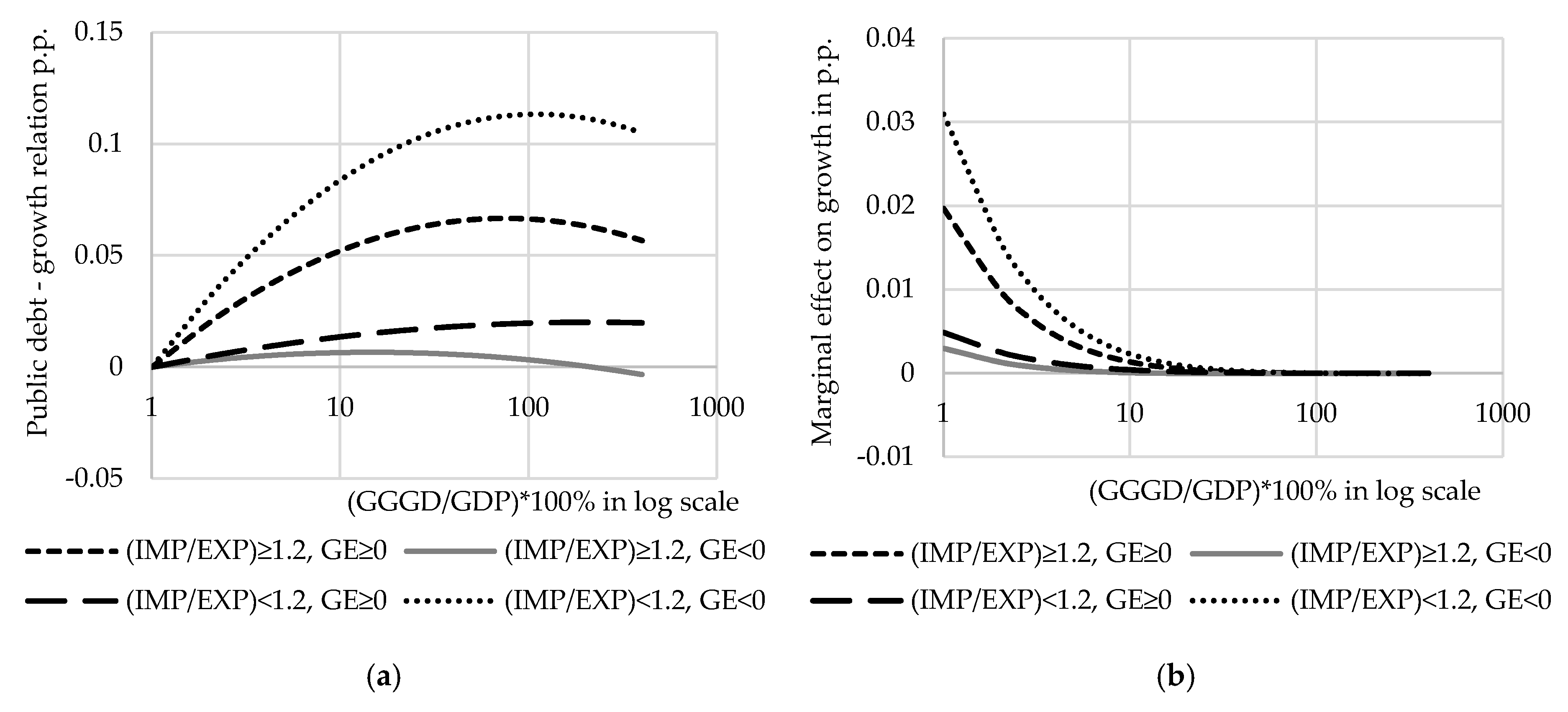
Figure 1 shows estimated relation and marginal debt effect on growth in sub-samples.
3Estimated turning points in the direction of public debt-growth relationship range widely. We found that public debt to GDP ratio exceeding 15% already has negative effect on growth in countries with relatively high trade deficit and low government effectiveness. On contrary—high government effectiveness and low or no trade deficit might determine that even 200% of public debt to GDP ratio has no negative effect. Between these two extremes we have the group of countries with high government effectiveness and high trade deficit that has a turning point in public debt-growth relationship at about 75% of debt to GDP ratio. Meanwhile, countries with low or no trade deficit and low government effectiveness with a turning point in public debt-growth relationship when debt to GDP ratio exceed 111%. We found to some extent unexpected higher marginal effect in countries with low trade deficit and low government’s effectiveness compared with those countries where effectiveness is relatively high. These results suggest that there are other factors besides government effectiveness and trade balance, which might determine the debt impact on economic growth.
6. Robustness Check
To ensure that our general estimates are robust we performed a series of robustness checks changing specification of Equation (4) as well as using alternative estimators.
As discussed in
Section 4, another strategy employed in the literature is to control the direct effect of institutional quality on growth (
Megersa and Cassimon 2015;
Masuch et al. 2016;
Kim et al. 2017). Thus, the first step to check robustness of general estimations is to include government’s effectiveness (log[
ge+2.5]) indicator in growth equation (Equation (4)) to test whether trade deficit still has an effect on public debt-growth relationship when quality of governance is controlled. SYS-GMM estimates in
Table A3 (see
Appendix A) are for several groups of countries. Two of them are like in general estimations—(IMP/EXP) ≥ 1.2 and (IMP/EXP) < 1.2 and four additional—(IMP/EXP) ≤ 1 (trade surplus), 1 < (IMP/EXP) ≤ 1.2 (relatively low trade deficit), 1.2 < (IMP/EXP) ≤ 1.4 (average trade deficit) and (IMP/EXP) > 1.4 (huge trade deficit).
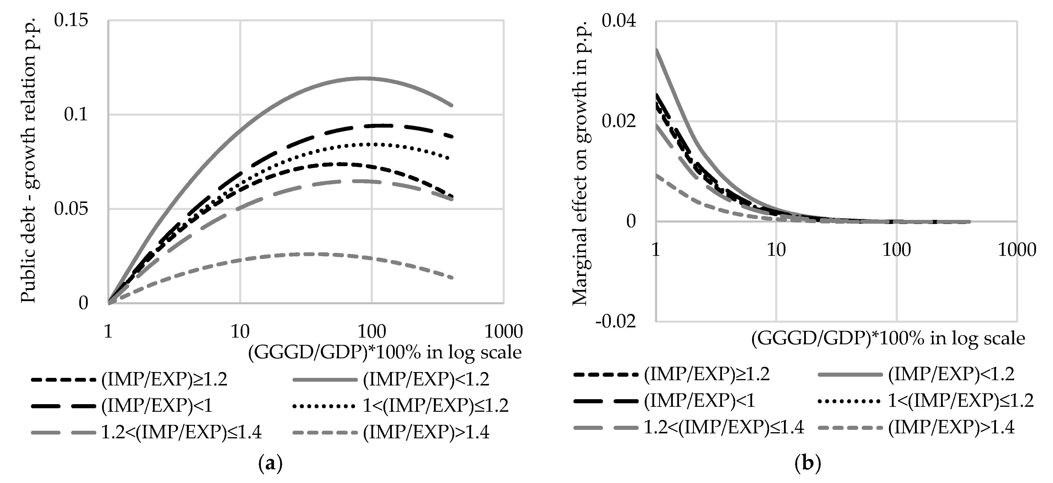
Figure 2 shows estimated public debt-growth nexus and marginal public debt effect on growth in sub-samples when government effectiveness is controlled.
4The estimates show that the bigger the trade deficit is the smaller public debt to GDP ratio will probably cause negative effect on growth.
To check the robustness of the general estimates we estimated Equation (4), using 10-year growth averages ({log[
gdpi,t+10/
gdpi,t]}/10) instead of 5-year averages. Calculating averages for 1996–2006, 1997–2007 and so on up to 2006–2016 extremely reduces the number of observations. SYS-GMM estimates of Equation (4) with 10-year growth averages, as a dependent variable for initial groups of countries, are presented in
Table A4 (see
Appendix A).
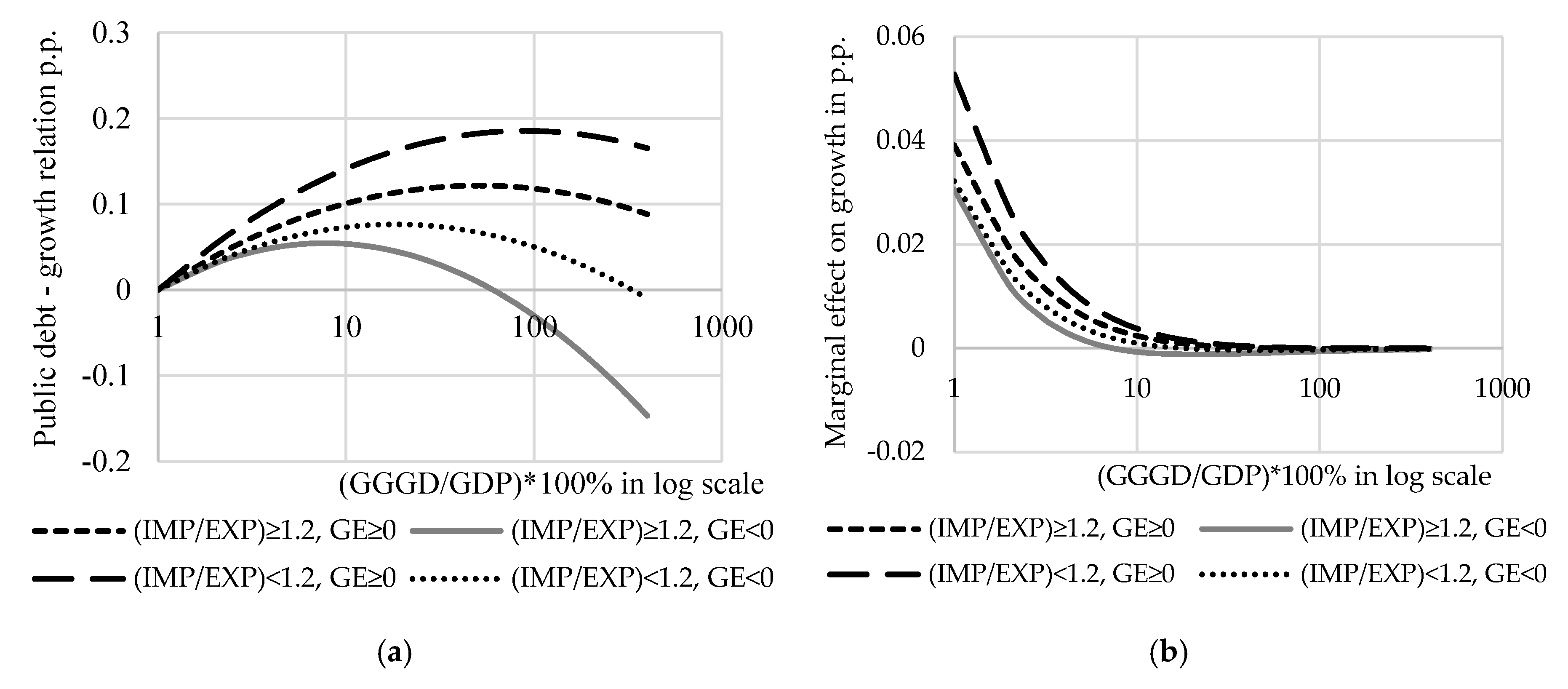
Figure 3 shows public debt-growth nexus and marginal debt effect on growth in sub-samples when growth is averaged over ten years
5.
The estimates using 10-year growth averages show quite the same pattern of public debt-growth relationship in terms of trade deficit and government effectiveness just with smaller public debt to GDP ratios as a turning point.
For the general estimations, we used the time averages of government effectiveness and trade deficit to assign countries to groups with high/low government effectiveness and high/low level of trade deficit. Nevertheless, the government effectiveness and level of trade deficit changed (in some of the countries quite sharply) over the analysed period. For the robustness check, we alternatively used the time-varying dummies. We constructed the dummy for high government effectiveness (
HGEDi,t), which is equal to unity if Government effectiveness indicator in a country
i during the year
t was above 0 and equal to zero otherwise. Using the same logic we also constructed the dummy for relatively high trade deficit (
HTDDi,t), which is equal to unity if import-export ratio in a county
i during the year
t was above 1.2 and equal to zero otherwise. We interacted time-varying dummies with debt variable to test whether public debt-growth relationship is conditioned on government effectiveness and trade deficit. Another motivation to estimate Equation (4), using interactions wh time-varying dummies, is that we did not find a clear inverted U-shaped form of public debt-growth relationship analysing the whole sample (unlike with estimations in separate subsamples, see
Table 1) what might suggest that this relationship is conditioned on other factors widely distributed across 152 countries over time. For this purpose, we modified Equation (4) by introducing interactions:
and
where
HGEDi,t and
HTDDi,t are the time-varying dummies for high government effectiveness and high trade deficit, respectively. In Equation (6)
β8 shows the effect of debt on growth in countries with low government effectiveness and
β8 +
β10 in countries with high one. In Equation (7)
β8 shows the effect of debt on growth in countries with low or no trade deficit and
β8 +
β11 in countries with high trade deficit. SYS-GMM estimates are reported in
Table 2.
With these estimates we found a highly statistically significant evidence that debt has a negative effect on growth in countries characterised as having low government effectiveness and rather strong statistical evidence that debt has a positive effect on growth in countries with high government effectiveness. The estimates suggest that the increase of debt to GDP ratio by 10 percentage points (p.p.) would lead to slower growth by about 0.72 p.p. in low government effectiveness countries and, on the contrary, would stimulate growth by 0.58 p.p. in high government effectiveness. These results might be interpreted that the certain level of government effectiveness is required to prevent negative debt impact on growth, however when this level is reached, government effectiveness is almost irrelevant for public debt-growth relationship. Also, our estimates provided statistically significant evidence suggesting positive debt-growth relationship in countries with low or no trade deficit and negative debt-growth relationship in countries with high trade deficit. The estimates show that increase in debt to GDP ratio by 10 percentage points would fasten growth by approximately 0.4 percentage points in a country characterised as having low trade deficit or trade surplus and would slow down growth by approximately 1 percentage point if one has relatively high trade deficit.
The last attempt to secure the rigorousness of our general estimates is to use alternative estimators as well as to change specification of Equation (4).
Bond et al. (
2001) argue that the pooled OLS and the LSDV estimators could be considered as the upper and lower bound of GMM estimator of dynamic growth model. If the GMM estimates are near to or below the LSDV ones, this could be due to that GMM estimates are downward biased what might be caused by a weak IV problem. In such case, the usage of SYS-GMM is suggested and its estimates should appear between OLS and LSDV. This insight is supported by
Hoeffler (
2002),
Nkurunziza and Bates (
2003) who empirically tested the augmented Solow growth model. The estimates of a model similar to Equation (4) by
Presbitero (
2008) showed that the SYS-GMM estimator is better compared to GMM because latter is highly downward bias. Despite of the aforementioned arguments in favour of SYS-GMM, it does not necessarily mean that it is not without drawbacks.
To change specification, we included regional dummies (from WDI) in all estimations and cross-sectional time-invariant dummies for legal origins, fractionalization measures for ethnic, language and religion and distance from the equator in OLS estimations. The estimation results are reported in
Table A5,
Table A6,
Table A7 and
Table A8 (see
Appendix A).
Table 3 summarizes the estimated turning points in public debt-growth relationship, using different estimation strategies as well as different specifications.
The turning point in the samples of countries with to some extent similar government effectiveness and level of trade deficit still varies depending on estimation technique but in most cases the variation is quite limited. All estimations confirm our hypothesis, that countries with better quality of governance and lower level of trade deficit have higher public debt threshold (turning point) level.
7. Discussion and Conclusions
The question, whether public debt is a means of or a burden on economic growth, is widely discussed in the scientific literature. The theory provides arguments how government borrowing and increasing debt can stimulate, impede or make no influence on economic development. There is quite a lot of empirical research devoted to the analysis of the impact the public debt makes on economic growth, despite this, the results are ambiguous. The growing number of recent research in this field confirms non-linear inverted U-shaped public debt-growth nexus, however estimated public debt threshold level (or turning point) above which relationship turns from positive to negative, varies sharply across studies. This raises the need to analyse key factors, that might determine this debt threshold. While empirical evidence on this topic is rather scarce, there is a growing consensus institutional aspect to be one of the crucial factors, shaping debt impact on growth. Our findings are in line with
Woo and Kumar (
2015),
Marchionne and Parekh (
2015),
Ahlborn and Schweickert (
2018) and other studies, which suggest that debt-growth relationship has an inverted U-shaped form. The results confirm the idea that debt impact on economic growth might depend on institutional aspects as suggested, for example, by
Megersa and Cassimon (
2015),
Matemilola et al. (
2016),
Masuch et al. (
2016),
Kim et al. (
2017). However, sound institutions are not enough to prevent negative debt effect. Contrary to previous studies (
Jalles 2011;
Megersa and Cassimon 2015;
Matemilola et al. 2016), we found a significant U-shaped debt-growth link when estimated in the sample of countries with to some extent similar institutional quality as measured by government effectiveness. However, counties with high (low) government effectiveness can start facing negative impact at very different ratios of public debt to GDP. Depending on estimation technique, debt turning point varies from 46% to 229% and from 8% to 145% of GDP in countries with respectively high and low government effectiveness. Such extreme variation is sharply reduced if we take trade balance into account. Relaying on the trade and budget deficit relationship (“twin deficit” hypothesis) and expenditure multiplier effect, in this paper we assume that besides government effectiveness, a trade balance is another crucial factor determining debt threshold level. While exact debt turning point still varies depending on estimation method, when we consider both factors, that is, government effectiveness and trade balance, all specifications confirm the main idea, that countries with better quality of governance and lower level of trade deficit have higher debt threshold level.
We made an attempt to control endogeneity of public debt and other variables using SYS-GMM approach but the extent at witch we do this is limited to the approach itself. As previous contributions show, SYS-GMM estimator is not universally reliable and despite that our SYS-GMM estimates felt down between those for LSDV and OLS, this does not necessarily prove that they are absolutely unbiased. Although the omitted variable problem is reduced by using the SYS-GMM, we cannot eliminate the possibility that omitted variables to some extent made an impact on our research results. We did not explore other possible measures of countries’ institutional quality. Our findings do not give insights into all factors that may condition the effect of public debt on growth. It is possible, for example, that factors other than the government effectiveness and trade balance may explain the impact heterogeneity that public debt can have on growth.


