Article

Leaning against the Wind Policies on Vietnam’s Economy with DSGE Model

John von Neumann Institute, Vietnam National University, HoChiMinh 70000, Vietnam
*
Author to whom correspondence should be addressed.
Economies 2017, 5(1), 3; https://doi.org/10.3390/economies5010003
Submission received: 6 July 2016 / Revised: 16 November 2016 / Accepted: 17 November 2016 / Published: 18 January 2017
(This article belongs to the Special Issue Economic Development in Southeast Asia)

Abstract

:
The global financial crisis of 2007–2008 had a negative impact on many countries, including Vietnam. Many policies have been applied to stabilize the macro-economic indicators. However, most of them are based on old qualitative models, which do not help policy makers understand deeply how each one affects the economy. In this paper, we investigate a quantitative macro-economic approach and use leaning against the wind policies with the Dynamic Stochastic General Equilibrium model (DSGE) to find a better way to understand how policies stabilize the Vietnamese economy. Based on the framework of Gerali et al., we calibrate the hyper-parameter for Vietnam financial data and do the comparison between the standard Taylor rule and the cases in which we add asset price and credit elements. The results show that the credit-augmented Taylor rule is better than the asset-price-augmented one under the technology shock and contrary to the cost-push shock. Moreover, the extended simulation result shows that combining both asset-price and credit rules on the model is not useful for Vietnam’s economy in both types of shock.
JEL Classification:
C68; E00; E12; E52; E62

1. Introduction

Monetary policy is an extremely important macro-economic regulation of government in a market economy. It is a process by which the authority of a country controls the money supply and tends to target an expected inflation rate or interest rate to ensure price stability, general trust in the currency and lowering the unemployment rate. Moreover, it also maintains predictable exchange rates with other currencies. Monetary economics provides insight into how to craft optimal monetary policy. However, the global financial crisis of 2007–2008 showed the lack of policy execution in many countries. The economists realize that the monetary policies are deficient in considering some financial variables and parameters.
On the other hand, Vietnam was also partially affected by the crisis because the government was unable to predict that sudden situation and passive in executing monetary policies. By applying tight monetary policies in the early stage, they created huge shocks and negative effects to the currency markets, as well as commercial banks. The inflation rate and non-performing loan rate of Vietnam increased very greatly. Many policies were enforced, such as buying potentially billions of dollars of bad loans from the banks with official overdue debts (from 3% to 6%) [1]. All of them are based on qualitative models that do not help policy makers understand deeply how each one affects the economy. Therefore, we need another optimal solution to stabilize the Vietnamese economy. Although there are many studies about monetary policy, they are still missing quantitative models to evaluate correctly the effectiveness. In this paper, we investigate some macro-economic regulations and propose to use the Leaning Against The Wind (LATW) policy through the Dynamic Stochastic General Equilibrium (DSGE) model to find a suitable model for the Vietnamese economy. It was successfully applied in the European Central Bank. “Leaning against the wind” is defined as the Central Bank following a rule where the policy rate is adjusted not only in response to fluctuations of inflation and output, but also to the change of financial variables (asset prices, credit, etc.) (Leonardo and Federico, 2013) [2].
Lars E. O. Svensson (2014) [3] showed that the LATW was ineffective for Sweden. According to his paper, Sweden applied the LATW since 2010, and Riskbanks (Sweden’s central bank) realized that the inflation target was low and the unemployment was high. Similarly, Fabio Verona et al. (2014) [4] had evaluated the effective by using LATW policies for the U.S. market. These authors showed that both the credit-augmented Taylor rule and asset-price-augmented Taylor rule were effective with various shocks. Furthermore, some other studies regarding LATW, such as Lambertini et al. (2011) [5] and Christiano et al. (2010) [6], did not have financial frictions in banking and also did not perform a full grid-search analysis. Thus, in this paper, we simulate various scenarios of the combined Vietnam data to validate the model.
We make the following contributions: (i) calibrating hyper-parameters for Vietnam’s economy, where the data of the interest rate and GPD are collected from Quarters 1/1999–4/2014; (ii) inspired by the work of Gerali et al. (2010) [7], we extend their model by combining multiple economic policies. The results show that interest rate modeling when combining asset price and credit with the standard Taylor rule is not suitable for the Vietnamese market economy. This is a useful tool to identify problems and simulate solutions in operating the Vietnamese economy for policy makers. Besides, to estimate optimal parameters, we simulate each policy in many scenarios. When a shock happens, depending on the objectives that the Vietnamese economy is approaching, this tool will propose a specific suitable interest rate quantitatively, instead of qualitatively.
The rest of paper is organized as follows. Section 2 reviews the related literature. Section 3 presents the Dynamic Stochastic General Equilibrium (DSGE) model. Section 4 describes the main financial channels. Section 5 proposes our simulation method. Section 6 presents how parameters are calibrated, and Section 7 is the empirical results. Section 8 is the conclusion.

2. Literature Overview

The theoretical basis of the model in this paper originated from the two papers of Bernanke, Gertler and Gilchrist (1999) [8] and Lacoviello (2005) [9]. In that literature, they assumed that banks did not have any important role in credit transactions. However, in the real world, banks play a vital role in modern financial systems. This drawback induced the inaccurate prediction of the global crisis 2007. In order to overcome this weakness, Gerali et al. (2010) [7] added a new agent into the model “banks”.
Gerali stated that the banking sector in a Dynamic Stochastic General Equilibrium (DSGE) could clearly explain the role of banking inter-mediation in the transmission of monetary policy impulses and analyzed how shocks that originate in credit markets are transmitted to the real economy. On the other hand, compliance with the Basel Accords imposes capital requirements to exert banking activity. Gerali changed the standard model by adding credit frictions and borrowed constraints as in Iacoviello (2005) [9] and a set of real and nominal frictions as in Christiano et al. (2005) [10] and Smets and Wouters (2003) [11] with an imperfectly-competitive banking sector that collected deposits and then supplied loans to other agents subject to the requirement of using banking capital.
Based on main idea of Curdia and Woodford (2010) [12] combined with a simplified version of the above from Gerali et al. (2010) [7], the model included two transmission channel are: the bank lending channel with the presence of a target level for the bank’s leverage and the balance-sheet channel, which was referred from Lacoviello (2005) [9] and assumed that entrepreneurs’ borrowing capacity was linked to the value of the assets that they could pledge as collateral.
With regard to frictions in financial intermediates, many recent papers studied this issue, such as Bernanke and Gertler (2000, 2001) [13,14], Gilchrist and Leahy (2002) [15] and Iacovielllo (2005) [9]. The main feature of those was only to consider financial frictions from the borrowers’ side, but the credit-supply effects were still missing. Therefore, financial intermediates’ behavior was not expressed clearly. That was a reason why the framework was enriched by adding the leverage constraint into the banking sector. This would prevent the implication effect when shocks happen.
Related to the central bank’s policy interest rate, a paper from Curdia and Woodford (2009, 2010) [12,16] had modified a standard Taylor rule for a central bank’s policy interest rate to incorporate either an adjustment for changing interest rate spreads or a response to variations in the aggregate volume of credit. The results from that papers had shown that modified rules were better than the standard Taylor rule with different shocks. In our paper, besides the standard Taylor rule, there are two additional rules, the asset-price augmented rule and the credit augmented rule.
Moreover, Lambertini et al. (2011) [5] and Christiano et al. (2010) [6] did not have financial frictions in banking and did not perform a full grid-search analysis. Therefore, the paper’s contribution to the existent literature was an additional friction in banking and simulation to find out the optimal parameters for a desirable policy.

3. DSGE Model

We use the model that is from the papers of Gerali et al. (2010) [7] and Leonardo Gambarcorta et al. (2013) [2]. It introduces an important new agent, bank, into the DSGE model along with financial frictions (Iacoviello, 2005) [9]. This model is populated by five agents: households, entrepreneurs, banks, capital-good producers and retailers. Figure 1 describes how the model works.
The model starts with banks. They collect deposits from households and lend money to entrepreneurs. These loans depend on two financial frictions: one from the level of bank leverage and the other from the value of collateral. Then, entrepreneurs will make use of money to hire household labor and buy capital from capital-good producers. Finally, some retailers will buy the intermediate goods from entrepreneurs in a competitive market, brand them at no cost and sell them with a mark-up over the purchasing cost to households.

3.1. Households

Each household always maximizes its consumption and works less. Therefore, we assume the household utility function as below:
max c t P i , l t P i , d t P i E 0 t = 0 β P t log c t P i l t P i 1 + ϕ 1 + ϕ ,
subject to the budget constraint:
c t P ( i ) + d t P ( i ) w t l t P ( i ) + ( 1 + r t 1 i b ) d t 1 P ( i ) + J t R ( i ) ,
where c t P ( i ) is consumption, l t P ( i ) is labor supply, d t P ( i ) is bank deposits, which are paid at a rate equal to the policy rate r t i b , w t is the real wage and J t R ( i ) are the retailer’s profits.
Based on the budget constraint, it is easy to see that the household inflow is the wage that is paid by entrepreneurs, the interest receive from banks and the profits from selling to the other households. Therefore, the outflow, which includes consumption and deposits, has to be less than or equal to the inflow.
By using Lagrange multipliers, the First Order Conditions (FOC) for households are:
1 c t P ( i ) = E t β ( 1 + r t i b ) c t + 1 P ( i ) ,
l t P ( i ) ϕ = w t c t P ( i ) .

3.2. Entrepreneurs

Entrepreneurs maximize their utility function by consumption:
max { c t E ( i ) , l t P , d ( i ) , b t E E } E 0 t = 0 β E t log c t E ( i ) ,
subject to the budget constraint:
c t E ( i ) + ( 1 + r t 1 b ) b t 1 E E ( i ) + w t l t P , d ( i ) + q t k k t E ( i ) y t E ( i ) x t + b t E E ( i ) + q t k ( 1 δ k ) k t 1 E ( i ) ,
b t E E ( i ) m E q t + 1 k k t E ( i ) ( 1 δ k ) 1 + r t b ,
where c t E ( i ) is the entrepreneurs’ consumption, l t P , d ( i ) is the labor demand, k t E ( i ) is the entrepreneur’s stock of capital, q t k is the price of capital, y t E is the output of intermediate goods produced by entrepreneurs, which is the following Cobb–Douglas:
y t E ( i ) = A t E ( k t E ) ξ ( l t P , d ) ( 1 ξ ) ,
x t is the mark-up of the retailer sector, δ k is the depreciation of capital, b t E E ( i ) is the amount of the bank’s loans taken by the entrepreneurs, m E is a parameter that can be interpreted as the Loan-To-Value (LTV) ratio chosen by the banks and r t b is the interest rate on the bank’s loans.
The FOC are:
1 c t E ( i ) λ t 2 , E ( i ) = β E ( 1 + r t b ) c t + 1 E ( i ) ,
λ t 2 , E ( i ) m t E q t + 1 k 1 δ k 1 + r t b + β E c t + 1 E ( i ) q t + 1 k 1 δ k + r t + 1 k = q t k c t E ( i ) ,
( 1 ξ ) y t E ( i ) l t P , d ( i ) x t = w t ,
where the variable λ t 2 , E ( i ) is the second Lagrange multiplier on the borrowing constraint (and thus represented the marginal value of one unit of additional borrowing by the entrepreneurs), and 1 ξ is the output elasticity of labor in the production function.

3.3. Capital Good Producers

Because capital-good producers only sell fixed-capital to entrepreneurs, they maximize their utility function by the level of the price:
max I t + s E 0 s = 0 β s λ t + s 1 , E λ t 1 , E Q t + s k K t + s Q t + s k 1 δ k K t + s 1 P t + s I t + s ,
subject to:
K t + s = 1 δ k K t + s 1 + 1 κ i 2 I t + s I t + s 1 1 2 I t + s .
Perfectly-competitive firms buy last-period capital at price Q t k from entrepreneurs and I t units of final goods from retailers at price P t ; λ t 1 , E is the entrepreneurs’ marginal utility of consumption; q t k Q t k P t is the real price of capital; δ k is the rate of depreciation.
The FOC is:
1 = q t k 1 κ i 2 I t I t 1 1 2 κ 2 I t I t 1 1 I t I t 1 + β E E t λ t + 1 1 , E λ t 1 , E q t + 1 k κ i I t + 1 I t 1 I t + 1 I t 2 .

3.4. Retailers

Similar to capital-good producers, retailers only sell final goods to households, and so, they maximize the price according to the utility function:
max P t + s E 0 s = 0 β P λ t + s 1 , P λ t 1 , P P t + s ( i ) y t + s E ( i ) P t + s W y t + s E ( i ) κ P 2 P t + s ( i ) P t + s 1 ( i ) 1 2 P t + s y t + s E ,
subject to the demand derived from consumer’s maximization,
y t + s E ( i ) = P t + s ( i ) P t + s ϵ y y t + s E ,
where β P λ t + s 1 , P λ t 1 , P is the households’ stochastic discount factor, λ t 1 , P is the households’ marginal utility of consumption at time t, c t P is the current consumption, P t W is the wholesale price and P t ( i ) is the retail price; m k t y ϵ ϵ 1 , m c t E = 1 x t is the real marginal cost, and x t P t P t W .
The FOC is:
1 m k t y m k t y 1 + m k t y m k t y 1 m c t E κ P π t 1 π t + β P E t λ t + 1 P λ t P κ P π t + 1 1 π t + 1 Y t + 1 t = 0

3.5. Banks

Each bank j is composed of two units: a wholesale branch and a retail branch.
The wholesale branch: maximizes the following utility function subject to a balance-sheet constraint:
max { b t ( j ) , d t ( j ) } R t b b t ( j ) r t i b d t ( j ) θ 2 K t b ( j ) b t ( j ) ν 2 K t b ( j ) ,
s . t . b t ( j ) = d t ( j ) + K t b ( j ) .
In this Equation (18), we can see that the wholesale unit loans b t ( j ) with the wholesale loan rate R t b ( j ) by collecting deposits d t ( j ) from households, which are paying the interest rate set by the central bank r t i b . Besides, the banks have their own funds K t b ( j ) , which are accumulated from reinvested profits.
Moreover, ν is considered as the target leverage ratio and banks have to pay a certain cost for deviating from that target. In fact, the target leverage ratio is one of the tools of macro-prudential policy, which is applied to this paper. Whenever the bank deviates from that ratio, this leads to the losing of bank profits. Therefore, this will limit the ability of lending while the shocks are happening.
Using Lagrange multipliers for Equations (18) and (19), the FOC is:
R t b = r t i b θ K t b ( j ) b t ( j ) ν K t b ( j ) b t ( j ) 2 .
The retail branch: We assume that the retail banks operate in terms of monopolistic competition. Moreover, they buy wholesale loans, differentiate at no cost and resell to final borrowers. The utility function will be:
r t b = r t i b θ K t b ( j ) b t ( j ) ν K t b ( j ) b t ( j ) 2 + μ ¯ b ,
where r t b is the retail loan rate and the mark-up μ ¯ b is constant.

4. The Transmission Channels

This section will introduce two transmission channels: (i) a collateral channel; and (ii) a credit-supply channel.
The model includes two financial frictions: (i) entrepreneurs’ value of assets that affects their borrowing ability; and (ii) banks set up a target level and pay a cost if they deviate from it. Based on these financial frictions, we will present them as two additional transmission channels: (i) a collateral channel, which is linked to the borrowing constraint; and (ii) a credit supply channel, which is linked to the presence of a positively-sloped loan-supply, which shifts with changes in the policy rate and bank capital.
The collateral channel: The collateral channel operates based on the fluctuations of asset prices on the debtor’s balance-sheet condition, which influences the borrowing constraint. In this channel, the model assumed that β E < β P , and this lead to the households being net lenders and the entrepreneurs net borrowers, as shown in Iacoviello (2005) [9]. Moreover, the paper of Andres et al. (2010) [17] showed that: (i) the entrepreneurs always consume a fraction 1 β E of their net worth; (ii) the entrepreneurs’ capital is also a linear function of net wealth; the coefficient is time varying and depends on asset prices, the LTV ratio and the loan interest rate. The equations are:
c t E = 1 β E N W t E ,
K t = β E q t k χ t N W t E ,
where N W t E and χ t are the entrepreneurs’ net worth and the entrepreneurs’ leverage, respectively ( B t = χ t K t ). These two variables are defined as:
N W t E q t k 1 δ k K t 1 1 + r t 1 b B t 1 + ξ Y t x t ,
χ t m E q t + 1 k ( 1 δ k ) 1 + r t b .
From the above equations, we can draw a few main ideas about this model as follows:
(i)
Equation (25) shows that the leverage ratio depends positively on the parameter m E and future asset prices q t + 1 k and negatively on the loan interest rate.
(ii)
The asset prices and the lending rates from (25) have a crucial impact on the entrepreneurs’ net worth, which influences simultaneously both consumption and investment decisions described through Equations (22) and (23).
(iii)
Equations (23)–(25) can be interpreted as using past net worth, which is the basis to borrow money from intermediates with a given fraction in order to buy future capital.
(iv)
In detail, from Equations (22) and (24), we see that the current level of asset prices ( q t k ) has a positive relation with net worth; it has a positive impact on consumption, as well. Hence, the increase of the current level of asset prices will induce the increase of consumption. Conversely, the impact of the current level of asset prices on investment (Equations (23)–(25)) is ambiguous, because the positive effect of the current level of asset prices will be counteracted by the negative effect of leverage, which is considered as the cost of purchasing new capital. Expectations on future asset prices ( q t + 1 k ) positively impact investment (easy to see from Equations (23) and (25)), whereas the loan interest rate ( r t b ) negatively impacts both consumption and investment. Therefore, the increase of the loan rate will decrease net worth due to the increase of interest payments and the decrease of capital accumulation.
The credit-supply channel: Nowadays, in most countries, including Vietnam, banks have been implementing risk management following the rules of Basel II. Hence, this model assumed that credit intermediates manage supply conditions to the target capital to asset ratio 1. Whenever this ratio deviates, banks will tighten lending standards in order to limit lending amounts and bring this ratio back to the desired level. Equation (21) can be written in linear form as follows:
r ˜ t b = r ˜ t i b + θ ν 3 1 + r i b B ^ t θ ν 3 1 + r i b K ^ t b ,
Many of the main ideas we can draw are as follows:
(i)
The loan supply schedule B ^ t has a positive effect on the loan rate. The implication is that the increase of the lending amount will lead to a higher loan rate due to higher default risk.
(ii)
The multiplier of loan supply has a positive correlation for both the level of the bank’s target capital-to-asset ration (ν) and the cost for deviating from that target θ.
(iii)
From Equation (19), the level of bank capital has a positive effect on the loan supply, which depends positively on the bank’s profits. The capital will be accumulated through an increase in the bank’s profit; banks have numerous capital to lend, and this leads to the shift in the loan supply in the subsequent period. Moreover, the increase of bank profits will reduce the loan rate (in the subsequent period) for any given level of loans to the economy.
(iv)
In particular, the loan supply is inversely proportional to the level of the policy rate. Hence, whenever the central bank implements an easy policy, this will lead to the increase of loan supply. This feature is consistent with the existence of a bank-lending channel in the model.
In fact, the interaction between the credit-supply channel and the collateral channel will determine the equilibrium level of the interest rate. In detail, the changes in credit supply will impact the entrepreneurs’ net wealth, consumption and investment decisions. This will increase the implication effect, because the effect of different shocks increases or decreases the prices of assets as described in the collateral channel.

5. Simulations

5.1. Monetary Policies

In this section, we will test the efficiency of an LATW by empirical research with real data collected from the Vietnamese economy through the Dynare package. This answers the key question “Could LATW policies apply for Vietnam?”. Hence, first of all, we will introduce policies used to stabilize the economy. We assume that the central bank follows a general-form Taylor rule as follows:
r ˜ t i b = ρ i b r ˜ t 1 i b + 1 ρ i b ϕ π π ^ t + ϕ y Y ^ t + ϕ B B ^ t + ϕ q q ^ t k .
We take into account policies one-by-one; specifically, the three policies will be:
(i)
The standard Taylor rule:
r ˜ t i b = ρ i b r ˜ t 1 i b + 1 ρ i b ϕ π π ^ t + ϕ y Y ^ t .
(ii)
The Taylor rule augmented with asset prices:
r ˜ t i b = ρ i b r ˜ t 1 i b + 1 ρ i b ϕ π π ^ t + ϕ y Y ^ t + ϕ q q ^ t k .
(iii)
The Taylor rule augmented with credit:
r ˜ t i b = ρ i b r ˜ t 1 i b + 1 ρ i b ϕ π π ^ t + ϕ y Y ^ t + ϕ B B ^ t .

5.2. Shocks

To determine the policies that are desirable, we propose two shocks in the DSGE model: (i) the technology shock; and (ii) the cost-push shock.

5.2.1. Technology Shock

The technology shock is a shock to total factor productivity, i.e., to the variable ( A t E ) in the production function:
y t E = A t E ( k t E ) ξ ( l P , d ) ( 1 ξ ) .
We assume that A t E follows an AR(1) process:
A t E = ρ A A t 1 E + ε t A .
We set ρ A = 0 . 95 , and the variance of A t E equals one percent, which are taken from Gerali et al. (2010) [7]. Technology shocks are events in a macroeconomic model that change the production function. The term shock is defined as a sudden change in the economy. A technology shock is when there is a sudden change in technology to either benefit or worsen economic activity. This type of shock has big effects on companies that are solely dependent on technology as their main source of labor or production, such as manufacturing plants or oil/energy extraction.

5.2.2. Cost-Push Shock

The second shock considered in this model is the cost-push shock (the so-called cost-push inflation), defined as a shock to the elasticity of substitution between varieties in the goods market. A situation that has been often cited of this was the oil crisis of the 1970s. Petroleum is so important to industrialized economies with no suitable alternative available, so a large increase in its price can lead to the increase in the price of most products, raising the inflation rate.
In this model, the cost-push shock is modeled through the firms’ mark-up m k t y as follows:
m k t y = ρ y m k t 1 y + ε t y .
We set ρ y = 0 . 50 , and the variance of ξ t is calibrated, so that the variance of m k t y equals one percent, which are taken from Gerali et al. (2010) [7].

5.3. Loss Function

In order to identify the desirable LATW policies in terms of macroeconomic stabilization, we consider assumptions about the central bank’s preferences. In particular, we assume that the central bank’s objective is the minimization of the weighted sum of the variance of inflation and output:
L o s s = V a r ( π ) + α V a r ( Y ) .
We set the weighting parameter α to vary within the range [0,2], i.e., we allow for a broad range of values for the relative weight of inflation versus output stabilization. The increase of value α shows that the central bank focuses on stabilizing output Y. For each value of α, we calculate the value of the loss function for each rule and then pick the minimum value as the best policy outcome attainable under that rule.

6. Calibration

In this section, we will introduce the specific parameters that are used for the simulation. A few of them are calibrated by the Vietnamese data. Due to the limit of the ability of the computer, we only simulate some scenarios to obtain a general view of the application of LATW policies in Vietnam. In particular, parameters ϕ y , ϕ B and ϕ q are changed from zero to two with a step size of one; parameter ϕ π is changed with the values being: 0.5, 1.5, 3 and 4.5. The value of the households’ discount factor β P is 0.996, which implies a steady-state policy rate of roughly 2% (annualized). The entrepreneurs’ discount factor β E is set at 0.975, which is from Iacoviello (2005) [9]. The inverse of the Frisch elasticity ϕ is set at one (Gali, 2008) [18]. The share of capital in the production function (α) and the depreciation rate of physical capital ( δ k ) are set at 0.20 and 0.05, respectively, in order to match the investment-to-GDP ratio and the entrepreneurs’ share in consumption in Gerali et al. (2010) [7]; which equal 0.11 and 0.09, respectively. The elasticity of substitution across goods ε y is set at six, implying that the mark-up in the goods market ε y ε y 1 is 1.20. The degree of price stickiness κ p is set at 28.65, the value estimated by Gerali et al. (2010) [7]. As mentioned, the degree of monetary policy inertia is set at 0.77. As regards the parameters related to the financial frictions/banking sector, we follow Gerali et al. (2010) [7]. The LTV ratio set by the banks m E is set at 0.35, which is similar to what Christensen et al. (2007) [19] estimated for Canada and to the average ratio of long-term loans to the value of shares and other equities for non-financial corporations in the European area, as in Gerali et al. (2010) [7]. The target capital-to-asset ratio ν, the cost for managing the bank capital position δ b and the elasticity of substitution across loan varieties ϵ b (which determines the steady-state loan spread) are set at 9%, 0.049 and 3, respectively, as in Gerali et al. (2010) [7]. The bank capital adjustment cost θ equals 11, the estimated value in Gerali et al. (2010) [7].

7. Empirical Results

In this section, we discuss some results obtained by simulating in different scenarios, including technology shock and cost-push shock. For each scenario, we try four groups of policies. The first one is the Taylor rule, which only takes into account the interest rate and inflation rate parameters. This is the baseline or standard rule of our model. We further augment the standard rule with the following extra parameters: asset price, credit and both of them. The simulation results will be shown in the next sections.

7.1. Scenario 1: Technology Shock

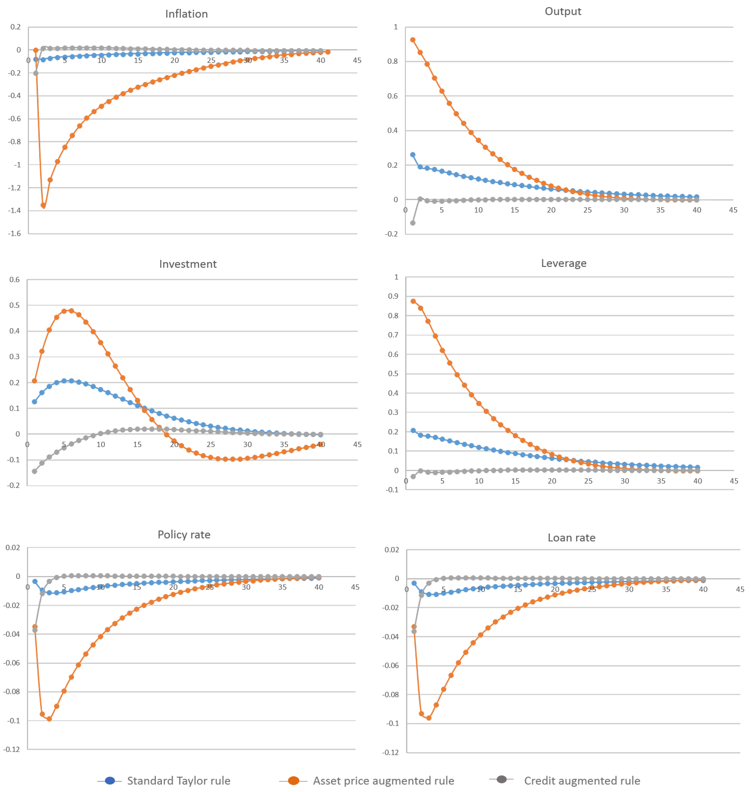
Figure 2 shows that, after the technology shock, the increase in asset prices has led to the relaxation in the borrowing constraint of the entrepreneurs. Furthermore, under the standard rule, both the policy and the loan rate decrease. The decrease of the loan rate increases entrepreneurs’ lending demand, which increases banks’ balance-sheet and leverage (the increase in leverage has activated the credit-supply channel), which also induces the strong increase of the investment and consumption of entrepreneurs and households (due to higher wages).
Under the credit-augmented Taylor rule, on the contrary, both the policy rate and loan rate increase when the shock hits the economy. This shows the counteracting effect of leaning against the wind, whereby the central bank could prevent the over-extension of banks, as well as the amplification of asset values. In addition, the tightening of monetary policy has affected the increase of bank lending rates, which induces a smaller expansion of bank leverage. In turn, in this case, borrowers’ financing conditions improve significantly less (because the increase of the loan rate has decreased the entrepreneurs’ net worth), so that the increase in investment, consumption and output is lower. Thus, the reduction of output volatility under leaning against the wind has lost both the amplification effect of the traditional collateral channel and the credit supply channel.
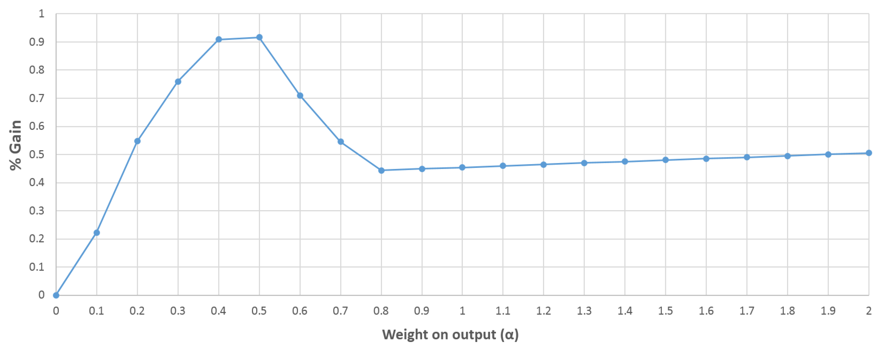
Meanwhile, under the asset-price-augmented rule, both the policy rate and loan rate significantly decrease; this has led to the strong increase of output, which the implication effect did not dampen. Thus, the asset-price Taylor rule proved virtually ineffective. Looking at Table 1, the asset-price-augmented rule is ineffective; the optimal parameter of ϕ q is zero. On the contrary, the credit-augmented rule is a desirable policy after technology shock; we can see this clearly through Figure 3. From Figure 3, we can see that the gains 2 under the standard Taylor rule and the credit-augmented rule are positive numbers; this shows that the credit-augmented rule is better than the standard Taylor rule. Moreover, we can see from this figure that the gains increase as α increases. To explain this, in this model, the increase in output (due to the positive shock) has increased the entrepreneurs’ net worth (Equation (24)). The borrowing conditions is loosened, and entrepreneurs will borrow more money, which leads to the rapid expansion of credit. Hence, the credit-augmented rule is effective in this case.

7.2. Scenario 2: Cost-Push Shock

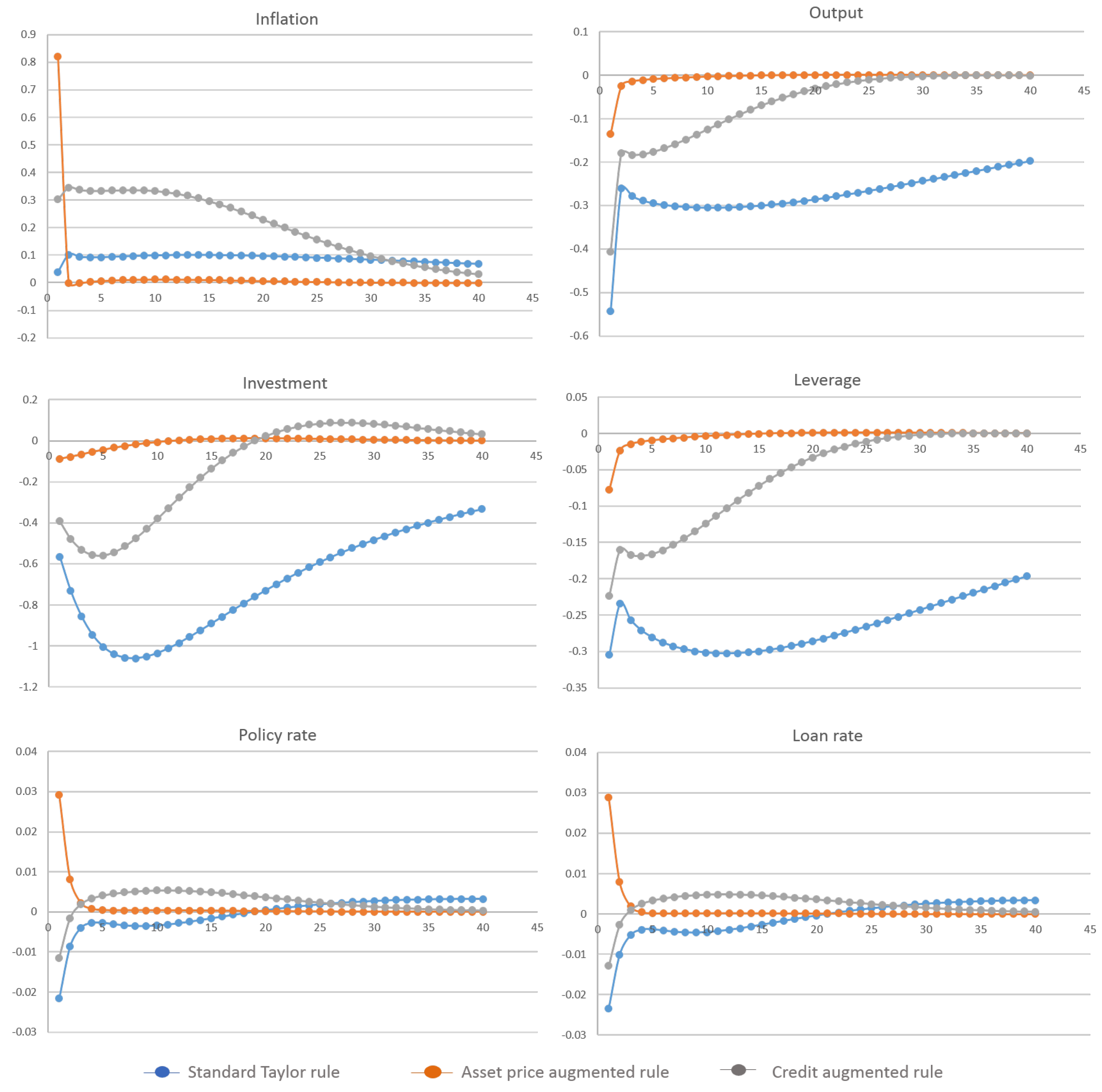
From Figure 4, after an adverse inflation shock, the output significantly decreases under the standard rule compared to under the asset price-augmented rule. We see that the different rules have led to the difference in output volatility. Under the standard rule, both the policy and the lending rates rise over time; the banks’ balance sheets (leverage) will be reduced; leading to a sharp deterioration of entrepreneurs’ financing conditions and, hence, the fall in investment.
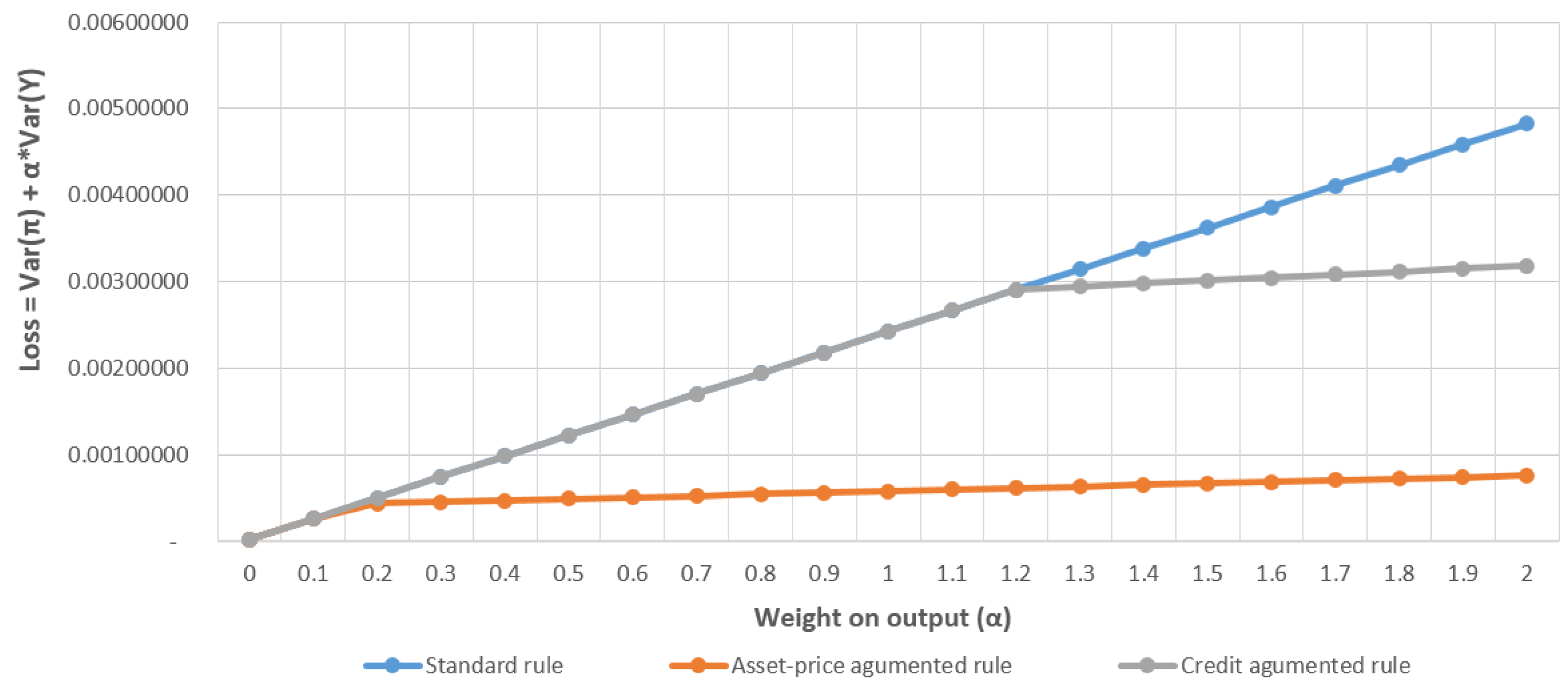
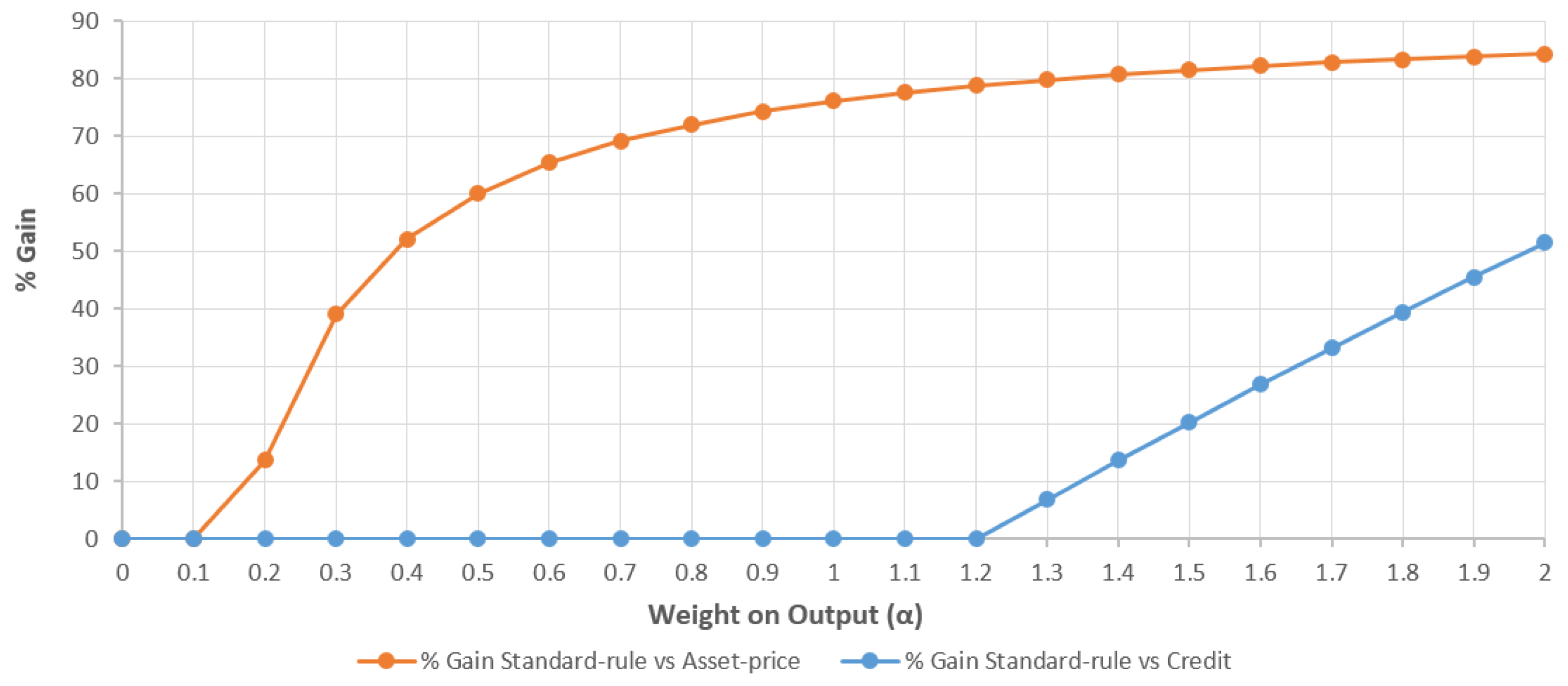
Under the rule including asset prices, instead, both the loan rate and policy rate are larger at first, but decrease later; the monetary policy is eased on impact; this has contributed to limiting the deterioration of the entrepreneurs’ financing conditions by sustaining banks’ balance sheets and avoiding a major disruption of credit supply. The output and investment increase, as well. We confirm that through Figure 5 and Figure 6, the loss function value is smaller, and the gain is larger under the asset price-augmented rule than others. The value of α is larger, and the gain and the loss under the asset-price-augmented rule is better (more detail in Table 1 and Table 2). This shows that the LATW policies are effective at stabilizing the economy for various shocks.
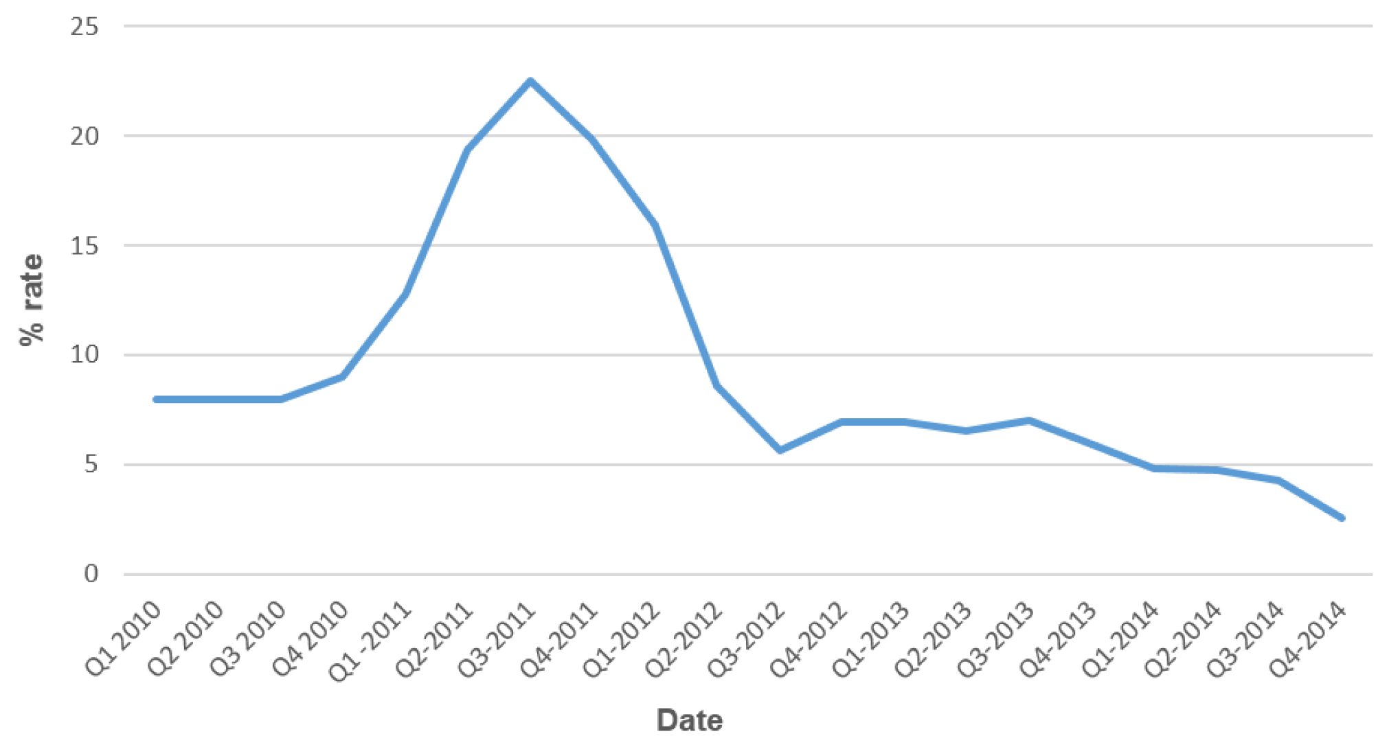
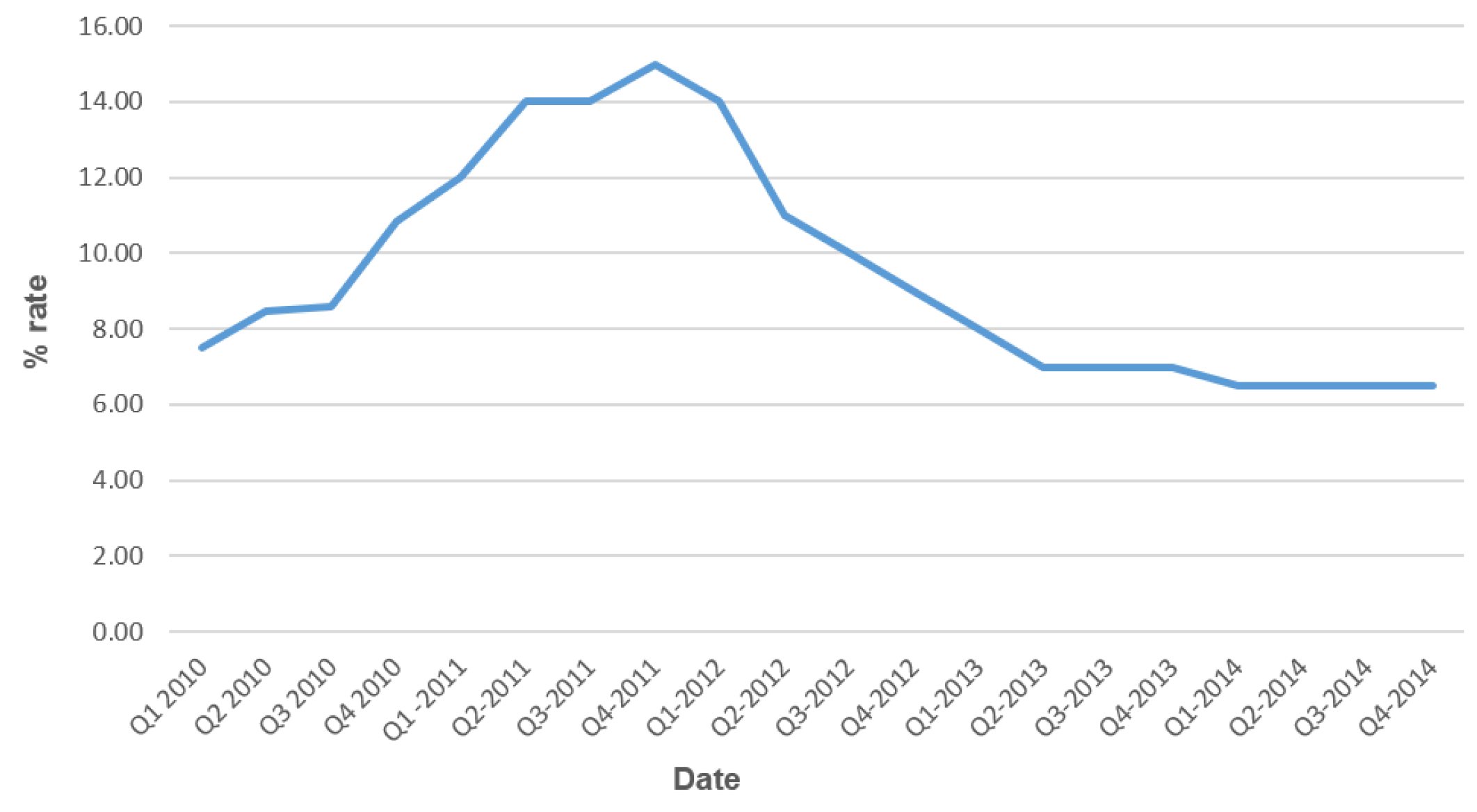
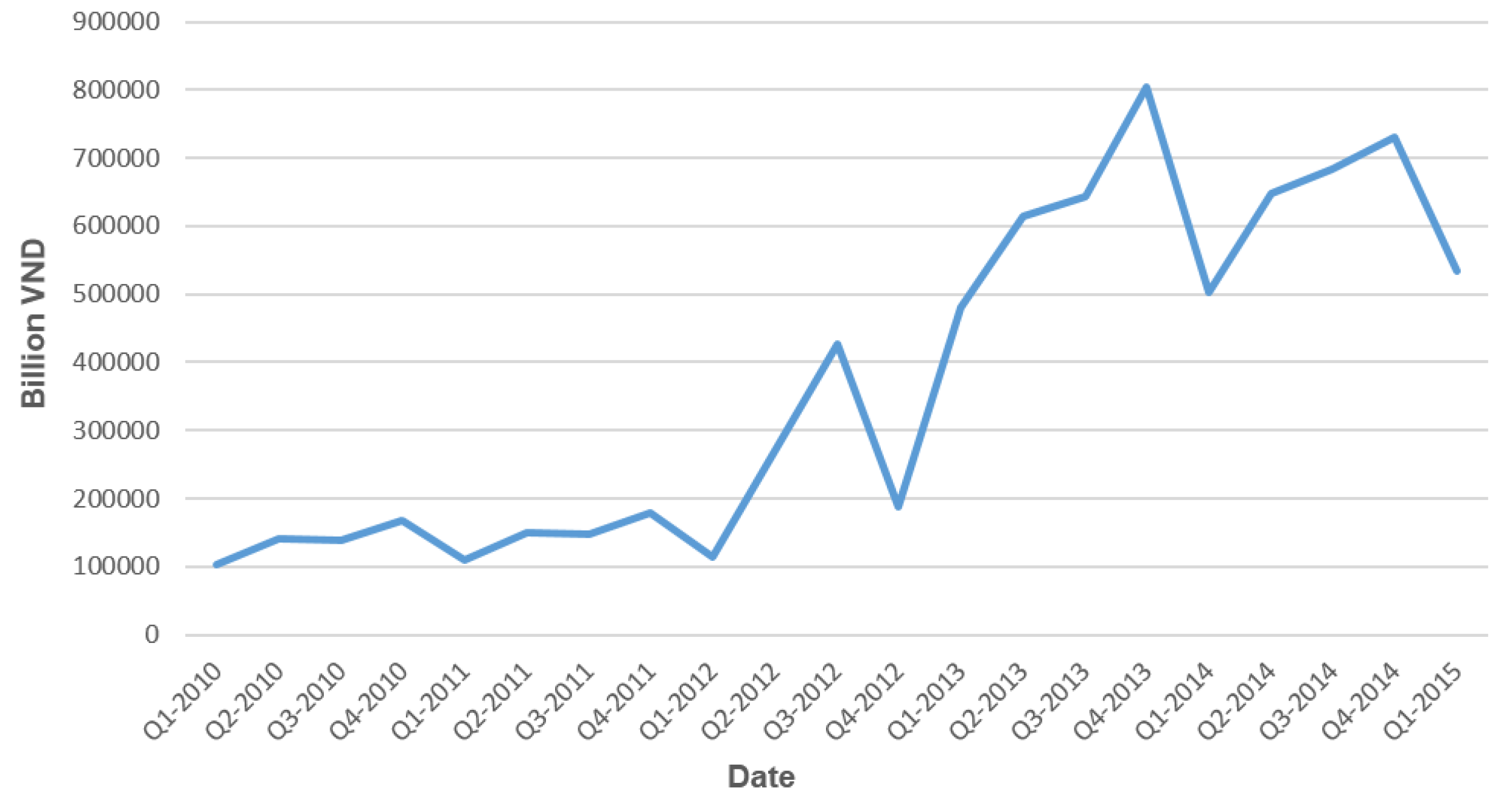
According to the report of the General Statistics Office of Vietnam, the increase of oil price from 17% up to 24% and electricity prices up to 15.2% in March 2011 led to the inflation increases from 12.8% in the first quarter of 2011 (up 60% compared with the prior year) up to 19.83% in the fourth quarter of 2011 (up 38.35% compared with the prior year) as described in Figure 7, also the policy rate increases from 12% in the first quarter of 2011 (up 59.97% compared with the prior year) to 15% in the fourth quarter of 2011 (up 120.28% compared with the prior year), as described in Figure 8. However, the goal of the Vietnamese monetary policy is to curb inflation through controlling the interest rate. Thus, GDP slowly grew from the first quarter of 2011 to the first quarter of 2012, as in Figure 9. The results realistically explained the responses described in Figure 4.

7.3. Combining Asset Price and Credit

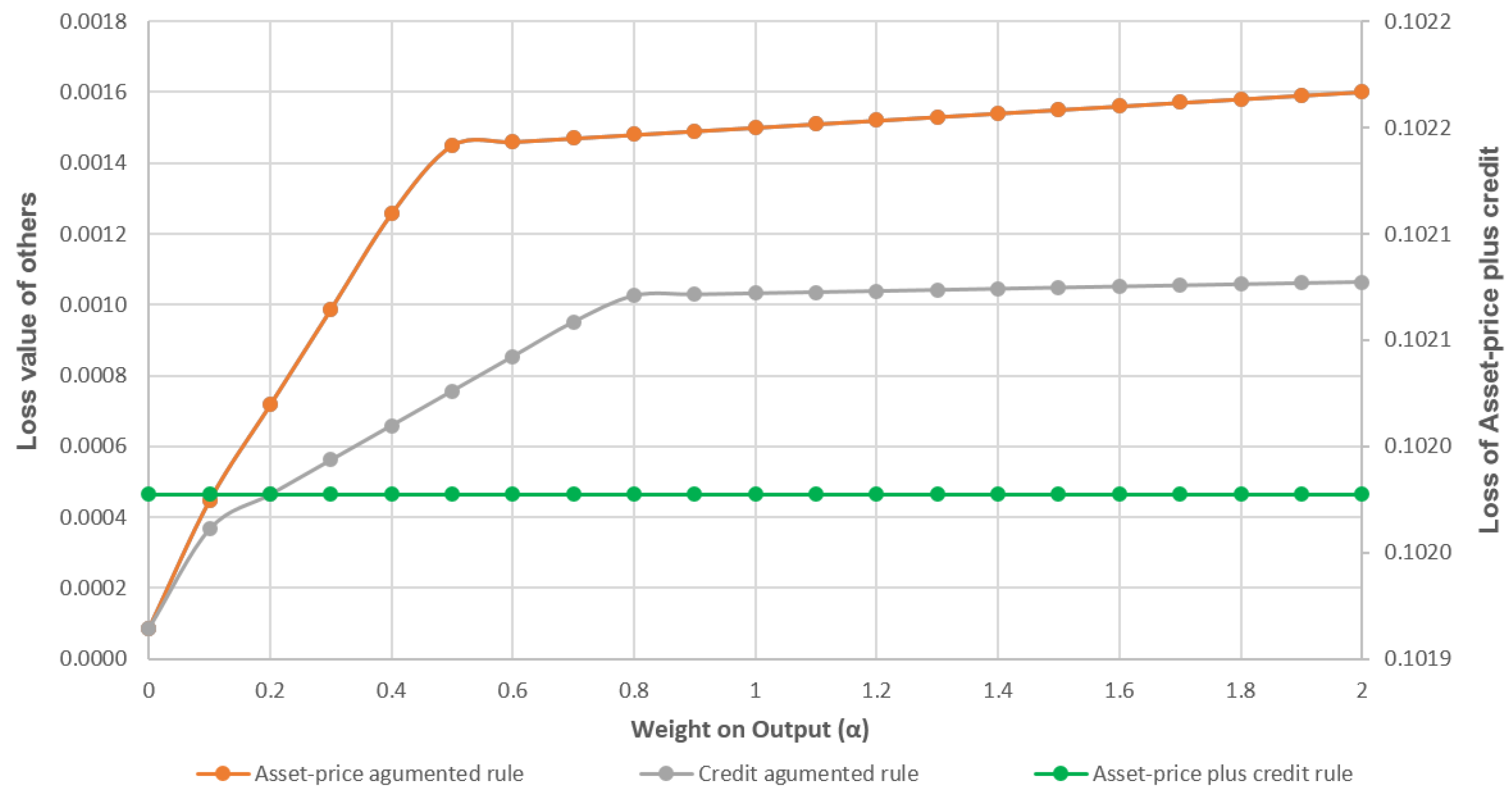
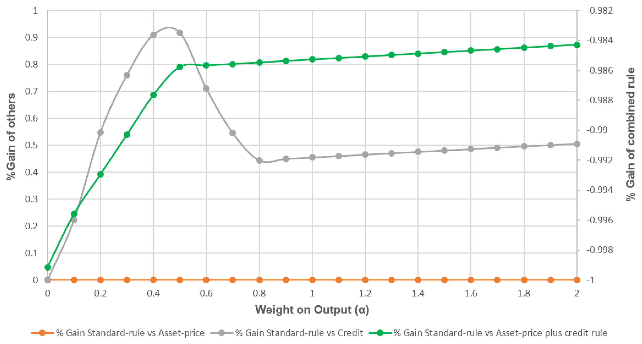
From the previous results, a question we investigated in this paper is: can combining both asset price and credit improve the model in both scenarios of technology shock and cost-push shock? In the scenario of technology shock, even combined with the two new policies, the Taylor rule still has the best result with the lowest loss. Note that, in Figure 10, the loss functions of the credit-augmented rule and standard rule are identical. The loss function of the asset price and credit rule is drawn in the secondary axis of the figure. In order to compare with the standard Taylor rule, we compute the percentage of gain after the technology shock, as shown in Figure 11.
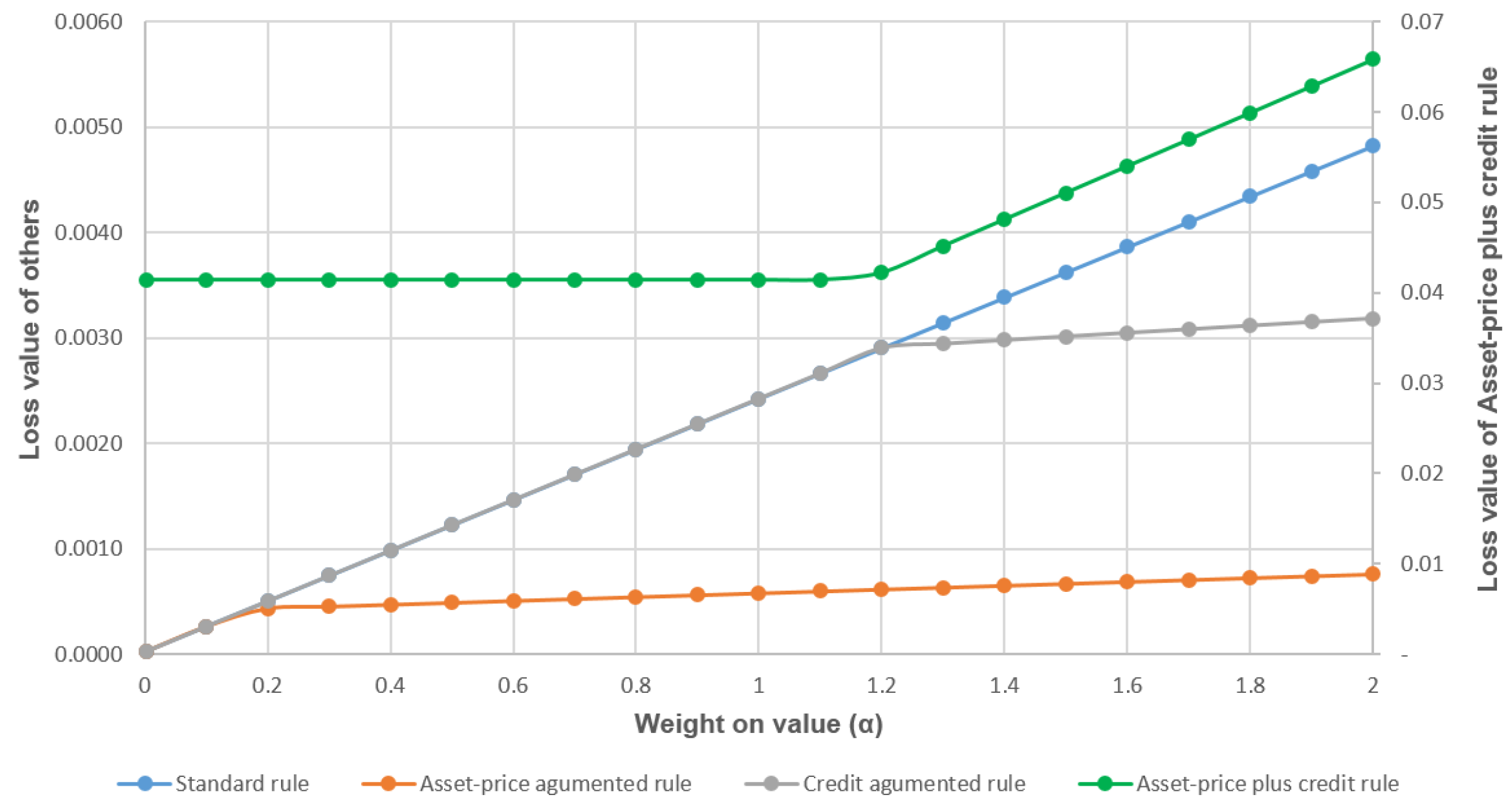
In the scenario of cost-push shock, the asset price-augmented rule is still the best rule with the lowest loss. Figure 12 shows the loss functions of the four methods. Similar to Figure 10, the loss function of the asset price and credit rule is drawn in the secondary axis.
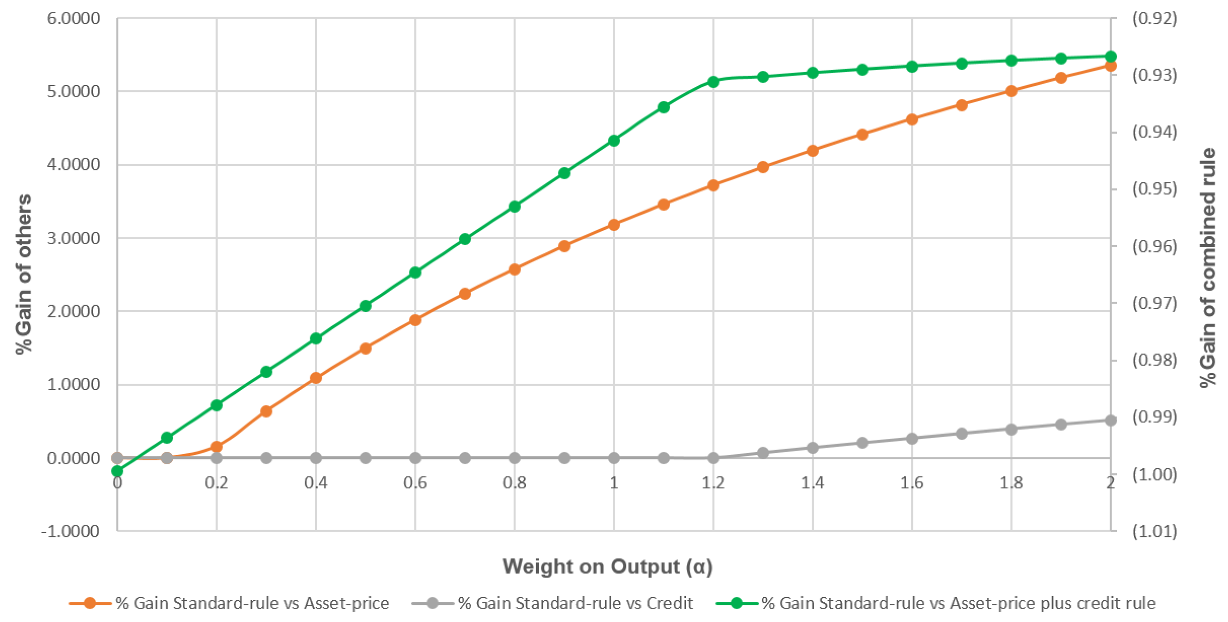
The standard Taylor rule has been used for a long time in stabilizing the economy. For example, in the context of a positive shock, it has proven effective for the economy of Vietnam. When a negative shock occurs, the asset-price-augmented rule proved to be more effective. However, the combination of the asset-price and credit rule on the model is shown not to be useful for Vietnam’s economy in both types of shock. This can be seen in Figure 13.

8. Conclusions

This paper showed the effectiveness of LATW policies for application to Vietnam. The Vietnamese monetary policy for stabilizing the economy through controlling the interest rate based on output and inflation is not enough. To improve significantly the performance of the economy, the Vietnam Central Bank needs to consider adding to the factor the amount of the loan for the technology shock (or the positive shock) or the factor of the entrepreneurs’ asset price for the cost-push shock (or negative shock).
Interestingly, the results of the model applied on the Vietnamese economy are similar to the results of the model by Gerali et al. (2010) ([7]) applied to the European economy. The results showed that output grew very slowly after the cost-push shock (the increase of oil and electricity prices) in the year 2011; this happens to coincide with the considered model. Thus, the LATW policy could be a desirable policy to apply in the future to stabilize and improve Vietnamese economy performance.

Acknowledgments

This research is funded by Vietnam National University Ho Chi Minh City (VNU-HCM) under Grant Number B2015-42-01.

Author Contributions

All authors contributed equally to the paper.

Conflicts of Interest

The authors declare no conflict of interest.

References

  1. D.N. Anh. “Non-Performing Loans—Case Study in Vietnam: Causes, Consequences, and Effects.” Bachelor’s Thesis, Uppsala University, Uppsala, Sweden, 2014. [Google Scholar]
  2. L. Gambbarcorta, and F.M. Signoretti. Should Monetary Policy Lean against the Wind? An Analysis Based on a DSGE Model with Banking. Economic Working Papers, Bank for International Settlements; Oslo, Norway: Norges Bank, 2013, Volume 418. [Google Scholar]
  3. L.E.O. Svensson. Why Leaning against the Wind Is the Wrong Monetary Policy for Sweden. Stockholm, Sweden: Stockholm School of Economics, Stockholm University, 2014. [Google Scholar]
  4. V. Fabio, and M.F. Manuel. “Martins and Ines Drumond.” In Financial Shocks and Optimal Monetary Policy Rules. Helsinki, Finland: Bank of Finland, 2014, Volume 418. [Google Scholar]
  5. L. Lambertini, C. Mendicino, and M.T. Punzi. “Leaning against boom–bust cycles in credit and housing prices.” J. Econ. Dyn. Control 37 (2013): 1500–1522. [Google Scholar] [CrossRef]
  6. L. Christiano, C. Ilut, R. Motto, and M. Rostagno. Monetary Policy and Stock Market Booms. Cambridge, MA, USA: National Bureau of Economic Research, 2010. [Google Scholar]
  7. A. Gerali, S. Neri, L. Sessa, and F.M. Signoretti. “Credit and Baking in a DSGE model of the Euro Area.” J. Money Credit Bank. 42 (2010): 44–70. [Google Scholar] [CrossRef]
  8. B.S. Bernanke, M. Gertler, and S. Gilchrist. “The Financial Accelerator in a Quantitative Business Cycle Framework.” In Handbook of Macroeconomics. Edited by J.B. Taylor and M. Woodford. Amsterdam, The Netherland: North-Holland, 1999, pp. 1341–1393. [Google Scholar]
  9. M. Iacoviello. “House Prices, Borrowing Constraints and Monetary Policy in the Business Cycle.” Am. Econ. Rev. 95 (2005): 739–764. [Google Scholar] [CrossRef]
  10. L. Christiano, M. Eichenbaum, and C. Evans. “Nominal Rigidities and the Dynamic Effects of a Shock to Monetary Policy.” J. Political Econ. 113 (2005): 1–46. [Google Scholar] [CrossRef]
  11. F. Smets, and R. Wouters. “An Estimated Dynamic Stochastic General Equilibrium Model of the Euro Area.” J. Eur. Econ. Assoc. 1 (2013): 1123–1175. [Google Scholar] [CrossRef]
  12. V. Curdia, and M. Woodford. “Credit Spreads and Monetary Policy.” J. Money Credit Bank. 42 (2010): 3–35. [Google Scholar] [CrossRef]
  13. B. Bernanke, and M. Gertler. Monetary Policy and Asset Price Volatility. Cambridge, MA, USA: National Bureau of Economic Research, 2000. [Google Scholar]
  14. B.S. Bernanke, and M. Gertler. “Should Central Banks Respond to Movements in Asset Prices? ” Am. Econ. Rev. 91 (2001): 253–257. [Google Scholar] [CrossRef]
  15. S. Gilchrist, and J.V. Leahy. “Monetary Policy and Asset Prices.” J. Monet. Econ. 49 (2002): 75–97. [Google Scholar] [CrossRef]
  16. V. Cúrdia, and M. Woodford. Credit Frictions and Optimal Monetary Policy. Cambridge, MA, USA: National Bureau of Economic Research, 2015. [Google Scholar]
  17. J. Andrés, O. Arce, and C. Thomas. “Banking competition, collateral constraints, and optimal monetary policy.” J. Money Credit Bank. 45 (2013): 87–125. [Google Scholar] [CrossRef]
  18. J. Gali. Monetary Policy, Inflation, and the Business Cycle: An Introduction to the New Keynesian Framework. Princeton, NJ, USA: Princeton University Press, 2008. [Google Scholar]
  19. I. Christensen, P. Corrigan, C. Mendicino, and S. Nishiyama. An Estimated Open-Economy General Equilibrium Model with Housing Investment and Financial Frictions. Mimeo, Norway: Bank of Norway, 2007. [Google Scholar]
  • 1.According to Basel 2regulations, referred to as the Capital Adequacy Ratio (CAR).
  • 2.Gain is the percentage difference between the minimum loss under the standard Taylor rule and the augmented Taylor rule (100 × (Loss|STR − Loss|ATR) /Loss|STR). A positive number means that the augmented rule performs better than the standard one.
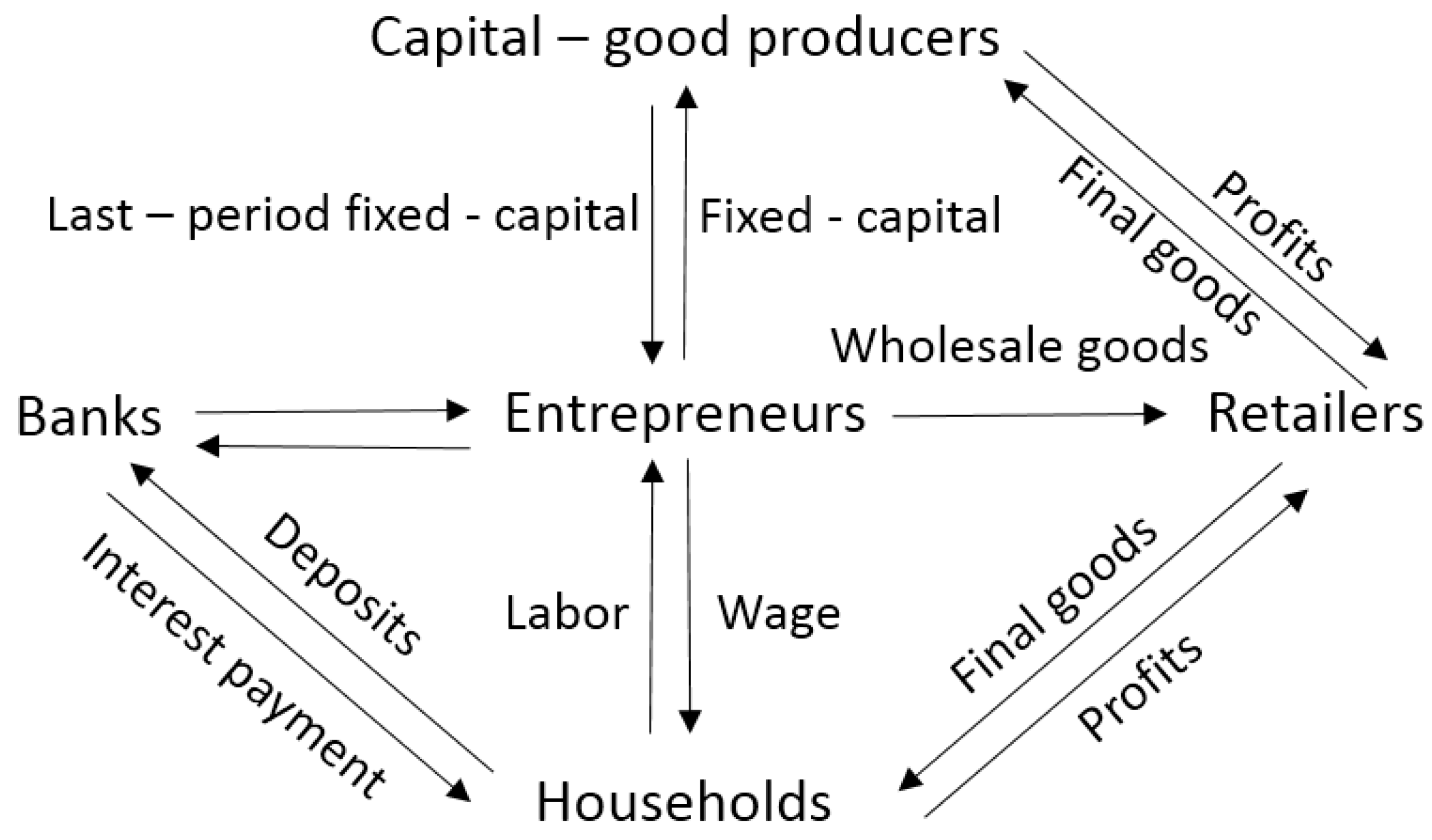
Figure 1. The DSGE model.
Economies 05 00003 g001
Figure 2. Impulse response functions after a technology shock.
Economies 05 00003 g002
Figure 3. % gain under the standard Taylor rule and that credit-augmented rule.
Economies 05 00003 g003
Figure 4. Impulse response functions after the cost-push shock.
Economies 05 00003 g004
Figure 5. Loss function of the Leaning Against The Wind (LATW) policies after the cost-push shock.
Economies 05 00003 g005
Figure 6. % gain after the cost-push shock.
Economies 05 00003 g006
Figure 7. Vietnamese inflation rate from the first quarter of 2010 to the fourth quarter of 2014.
Economies 05 00003 g007
Figure 8. Vietnam Central Bank policy rate from the first quarter of 2010 to the fourth quarter of 2014.
Economies 05 00003 g008
Figure 9. Vietnam GDP from the first quarter of 2010 to the first quarter of 2015.
Economies 05 00003 g009
Figure 10. Loss function of the LATW policies after the technology shock.
Economies 05 00003 g010
Figure 11. % gain after the technology shock.
Economies 05 00003 g011
Figure 12. Loss function of the LATW policies after the cost-push shock.
Economies 05 00003 g012
Figure 13. % gain after cost-push shock.
Economies 05 00003 g013
Table 1. Losses and gain under both the standard Taylor rule and the asset-price-augmented rule, after a technology shock.
Output Weight Standard Taylor Rule Asset-Price-Augmented Rule
α ϕ y ϕ π Loss ϕ pi ϕ y ϕ q LossGain
0 300.0008743 3000.000087430
0.1 0.500.00044837 0.5000.000448370
0.2 0.500.00071837 0.5000.000718370
0.3 0.500.00098837 0.5000.000988370
0.4 0.500.00125837 0.5000.001258370
0.5 1.520.00145042 1.5200.001450420
0.6 1.520.001460504 1.5200.0014605040
0.7 1.520.001470588 1.5200.0014705880
0.8 1.520.001480672 1.5200.0014806720
0.9 1.520.001490756 1.5200.0014907560
1.0 1.520.00150084 1.5200.001500840
1.1 1.520.001510924 1.5200.0015109240
1.2 1.520.001521008 1.5200.0015210080
1.3 1.520.001531092 1.5200.0015310920
1.4 1.520.001541176 1.5200.0015411760
1.5 1.520.00155126 1.5200.001551260
1.6 1.520.001561344 1.5200.0015613440
1.7 1.520.001571428 1.5200.0015714280
1.8 1.520.001581512 1.5200.0015815120
1.9 1.520.001591596 1.5200.0015915960
2.0 1.520.00160168 1.5200.0015915960
Output Weight Standard Taylor Rule Credit-Augmented Rule
α ϕ y ϕ π Loss ϕ pi ϕ y ϕ q LossGain
0 300.0008743 3000.000087430
0.1 0.500.00044837 3020.00036689718.17093026
0.2 0.500.00071837 3020.00046436435.35865919
0.3 0.500.00098837 3020.00056183143.15580198
0.4 0.500.00125837 3020.00065929847.60698364
0.5 1.520.00145042 3020.00075676547.82442327
0.6 1.520.001460504 3020.00085423241.51114958
0.7 1.520.001470588 3020.00095169935.28445765
0.8 1.520.001480672 3210.00102564430.73118152
0.9 1.520.001490756 3210.0010288530.98471514
1.0 1.520.00150084 3210.00103205531.23484182
1.1 1.520.001510924 3210.00103526131.48162978
1.2 1.520.001521008 3210.00103846631.72514543
1.3 1.520.001531092 3210.00104167231.96545341
1.4 1.520.001541176 3210.00104487732.2026167
1.5 1.520.00155126 1.5200.00104808332.43669662
1.6 1.520.001561344 3210.00105128832.66775291
1.7 1.520.001571428 3210.00105449432.89584378
1.8 1.520.001581512 3210.00105769933.12102595
1.9 1.520.001591596 3210.00106090533.34335472
2.0 1.520.00160168 3210.0010641133.56288397
Table 2. Losses and gain under both the standard Taylor rule and the credit-augmented rule, after the cost-push shock.
Output Weight Standard Taylor Rule Asset-Price-Augmented Rule
α ϕ y ϕ π Loss ϕ pi ϕ y ϕ q LossGain
0 1.500.00002388 1.5000.000023880
0.1 300.000264782 3000.0002647820
0.2 300.000504782 3010.00043582813.66015428
0.3 300.000744782 3010.00045381239.06780776
0.4 300.000984782 3010.00047179652.0913258
0.5 300.001224782 3010.0004897860.01084275
0.6 300.001464782 3010.00050776465.33518298
0.7 300.001704782 3010.00052574869.16039705
0.8 300.001944782 3010.00056171672.0414936
0.9 300.002184782 3010.0010288574.28960876
1.0 300.002424782 3010.000579776.09269617
1.1 300.002664782 3010.00059768477.5709983
1.2 300.002904782 3010.00061566878.80501876
1.3 300.003144782 3010.00063365279.85068599
1.4 300.003384782 3010.00065163680.7480659
1.5 300.003624782 1.5210.0006696281.52661319
1.6 300.003864782 3010.00068760482.20846609
1.7 300.004104782 3010.00070558882.81058531
1.8 300.004344782 3010.00072357283.346184
1.9 300.004584782 3010.00074155683.82570862
2.0 300.004824782 3010.0007595484.25752708
Output Weight Standard Taylor Rule Credit-Augmented Rule
α ϕ y ϕ π Loss ϕ pi ϕ y ϕ q LossGain
0 1.500.00002388 1.5000.000023880
0.1 300.000264782 3000.0002647820
0.2 300.000504782 3000.0005047820
0.3 300.000744782 3000.0007447820
0.4 300.000984782 3000.0009847820
0.5 300.001224782 3000.0012247820
0.6 300.001464782 3000.0014647820
0.7 300.001704782 3000.0017047820
0.8 300.001944782 3000.0019447820
0.9 300.002184782 3000.0021847820
1.0 300.002424782 3000.0024247820
1.1 300.002664782 3000.0026647820
1.2 300.002904782 0.5020.0006156680
1.3 300.003144782 0.5020.0029454066.769049836
1.4 300.003384782 0.5020.00297966813.59594425
1.5 300.003624782 0.5020.0030139320.267624
1.6 300.003864782 0.5020.00308245426.78932298
1.7 300.004104782 0.5020.00070558833.16604238
1.8 300.004344782 0.5020.00072357239.40256347
1.9 300.004584782 0.5020.00315097845.50345956
2.0 300.004824782 0.5020.0031852451.47310721