Spillover Effect of Food Producer Price Volatility in Indonesia

Abstract

Food price volatility is a persistent challenge in Indonesia, where agriculture is central to food security and rural livelihoods. While price transmission has been studied, little is known about how volatility spreads sub-nationally in archipelagic economies with fragmented infrastructure. This study applies a Dynamic Conditional Correlation GARCH (DCC-GARCH) model to monthly rural producer price data from 2009 to 2022 for six commodities: rice, chicken, eggs, chili, cayenne, and shallots. Results show that Java functions as the core volatility transmitter, with long-run conditional correlations exceeding 0.92 in Sumatra, 0.91 in Kalimantan, and 0.90 in Papua, reflecting strong and persistent co-movements. Even in low-production regions such as Maluku, significant volatility linkages reveal structural dependence on Java. Volatility clustering is particularly intense for perishables like chili and shallots. The findings highlight the need for spatially differentiated stabilization policies, including upstream interventions in Java and cooperative-based storage systems in outer islands. This study is the first to apply a DCC-GARCH framework to rural producer price data in an archipelagic context, capturing volatility transmission across regions. Its novelty lies in linking these spillovers with regional market dependence, offering new empirical evidence and actionable insights for designing inclusive and geographically responsive food security strategies.

1. Introduction

Commodity prices—particularly for agricultural goods—are widely recognized for their unpredictability. Unlike manufactured products, agricultural prices are especially sensitive to factors such as weather variability, shifting global market dynamics, and changes in government policy (Deaton & Laroque, 1992; Newbery, 1989; Pindyck, 2004). This volatility is not merely a matter of market fluctuation—it has real and often severe consequences for everyday life. In many developing countries, including Indonesia, where agriculture forms the backbone of the economy and serves as a primary livelihood source for millions, sudden food price changes can generate major disruptions. They can fuel inflation, destabilize trade balances, and place greater pressure on government spending through subsidies and social protection programs (Ivanic & Martin, 2008; Gilbert & Morgan, 2010). Understanding not just the magnitude of these fluctuations but also how they spread is therefore critical for policy design.

Of particular concern is the transmission of food price volatility across regions. A price shock in one area or commodity can ripple outward, affecting other regions and markets in what is commonly referred to as a spillover effect. These spillovers can intensify the impact of initial shocks, making it increasingly difficult for vulnerable communities to cope with rising costs. The risk of spillovers is heightened in closely connected and integrated markets, where price information and market signals travel rapidly. While this integration can improve market efficiency by aligning supply and demand, it also allows shocks to spread more swiftly and broadly (Conforti, 2004). This dual nature of market integration, offering both efficiency gains and heightened contagion risk, underscores the need to examine how volatility transmission operates in practice.

Among those most affected are smallholder farmers. Many rely heavily on farming as their sole income source, yet they lack access to financial tools or institutional support to manage the risks of volatile prices. When prices fall, their earnings shrink; when prices rise, input costs often become unaffordable. Price instability undermines their ability to plan, invest, and grow their businesses (Bellemare, 2014). Traders and other actors along the supply chain are also vulnerable, particularly in the absence of clear market signals about how price movements in one region may affect others (Nazlioglu et al., 2013). These vulnerabilities make it essential to pinpoint the specific channels and regions through which volatility is transmitted.

For policymakers, understanding when, where, and how price spillovers occur is essential for effective crisis management and market stabilization. If the inter-regional dynamics of food prices are well understood, governments can act pre-emptively by adjusting trade regulations, releasing buffer stocks, or providing targeted assistance to affected communities (Gilbert & Morgan, 2010). At the macroeconomic level, food price volatility poses risks to inflation control, fiscal stability, and broader economic resilience, particularly in agrarian economies where agriculture constitutes a significant share of GDP and employment (Baffes & Haniotis, 2016). In a country as geographically and economically diverse as Indonesia, such understanding must be grounded in subnational evidence rather than national averages alone.

Indonesia offers a compelling case study. As both a major producer and importer of key food commodities, the country’s markets are exposed to domestic and international price shocks. Climate events like El Niño and disruptions in global trade have historically led to large and sudden surges in food prices. These changes reverberate along the supply chain, influencing government policy, trade strategy, and long-term development planning. In Indonesia’s context, food price volatility is exacerbated by its archipelagic geography, which creates fragmented supply chains and amplifies the effects of local shocks. Volatility in one region—especially Java, the central hub for national food production and distribution—often spills over into other islands, including Sumatra, Kalimantan, and Sulawesi. For example, cayenne prices in Java have shown month-to-month fluctuations exceeding 30% during harvest failures, while distribution disruptions have triggered seasonal price spikes of over 50% for chili and shallots (BPS, 2022; KPPU, 2021). These patterns suggest that spatial transmission mechanisms are both significant and underexplored. These patterns suggest that volatility transmission is both substantial and geographically differentiated.

Despite growing awareness of these dynamics, most empirical studies of Indonesia’s food markets remain limited to national averages or isolated regional analyses. Much of the literature relies on static price convergence metrics or simple correlation analyses, offering limited insight into the time-varying and spatially heterogeneous nature of volatility (Barrett & Li, 2002). Consequently, there is still little understanding of how price instability originating in Java affects more peripheral regions, how these spillovers evolve, or how they differ across commodities. Addressing this evidence gap requires high-frequency, spatially detailed data and methods capable of capturing time-varying relationships.

This study addresses these empirical gaps by applying a Dynamic Conditional Correlation Generalized Autoregressive Conditional Heteroskedasticity (DCC-GARCH) framework (Engle, 2002) to assess the spatial spillovers of producer price volatility in Indonesia. Drawing on high-frequency monthly price data from 2009 to 2022, we focus on six widely consumed and historically volatile commodities: rice, chili, shallots, chicken, eggs, and cayenne. This multivariate approach allows us to capture dynamic co-movement structures and identify volatility transmission hubs—particularly with the central role of Java as a systemic risk node. By linking rigorous econometric modeling with granular rural data, our approach provides an empirical foundation for spatially targeted policy interventions.

By identifying these volatility linkages, our study provides new empirical evidence on the geography of food market volatility in Indonesia. The findings offer critical insights for designing geographically differentiated stabilization policies and underscore the importance of improving inter-island logistics, decentralizing supply chains, and building regional food reserves. Ultimately, understanding the spatial dynamics of price volatility is vital for enhancing food market resilience, protecting livelihoods, and ensuring national food security.

The primary research gap addressed in this study is Indonesia-specific. Most prior work has examined price levels or pass-through effects, with limited evidence on time-varying volatility transmission across regions using rural producer prices. A secondary gap is global in scope: little is known about spatial volatility spillovers in archipelagic, domestically oriented food systems, where maritime logistics constraints and seasonal production patterns influence transmission dynamics. This study addresses the Indonesia-level gap directly and contributes to the broader literature by providing empirical evidence from an archipelagic setting using granular rural data.

This study makes an original contribution by applying a Dynamic Conditional Correlation GARCH framework to rural producer price data in Indonesia, an archipelagic economy where infrastructure and production capacity vary widely across regions. The originality lies in using this approach to capture time-varying volatility spillovers across multiple key commodities, a dimension rarely addressed in the existing literature. The novelty is twofold: first, it provides empirical evidence on spatial volatility dynamics that reveal the dependence of outer islands on Java’s markets; second, it links these findings with regionally tailored policy implications. By filling this gap, the study advances the literature on food price volatility and offers practical insights for designing more inclusive and geographically responsive food security strategies.

2. Literature Review

Understanding food price volatility and its spatial transmission requires a multidisciplinary lens that draws from agricultural economics, spatial econometrics, and food policy. While classical price theory assumes that price adjustments across space occur efficiently in well-integrated markets, real-world conditions-marked by trade frictions, infrastructure deficits, and frequent supply shocks-can render price volatility spatially persistent and asymmetric (Ravallion, 1986; Anderson & van Wincoop, 2003).

Empirical evidence from developing countries shows that price volatility often stems from fragmented supply chains and uneven market access. Minten and Kyle (2014), for example, document significant intra-annual price swings in Indian vegetable markets, largely driven by perishability and logistical bottlenecks. In Ethiopia, Haile et al. (2019) show that short-term food price shocks are exacerbated by inadequate infrastructure, limiting farmers’ ability to respond to price signals. In Indonesia, Rahmawati et al. (2019) analyze spatial integration in shallot markets and reveal weak price pass-through between Java and outer islands, though their work does not address the dynamic nature of volatility or time-varying spatial spillovers.

To better quantify price risk, volatility models such as the Autoregressive Conditional Heteroskedasticity (ARCH) and Generalized ARCH (GARCH) frameworks have become standard tools in commodity market analysis (Engle, 2002). However, their application to rural markets in Indonesia remains limited. More advanced models like the Dynamic Conditional Correlation GARCH (DCC-GARCH) are particularly useful in capturing co-movement and time-varying volatility across multiple regions and commodities. Smiech et al. (2019) and Tsiboe et al. (2025), for instance, use DCC-GARCH to identify spatial volatility spillovers in agricultural markets, demonstrating the model’s power to uncover evolving interdependencies. Yet, such approaches are rarely applied using disaggregated, high-frequency rural price data in archipelagic economies like Indonesia.

This study responds to that gap by employing a DCC-GARCH framework to analyze spatial volatility spillovers using monthly producer price data from 2009 to 2022 for six key food commodities in Indonesia. The novelty of this approach lies in capturing not only the level of price integration but also the dynamic volatility linkages between regions, with a specific focus on Java’s role as a systemic volatility hub. This contributes new empirical evidence to the underexplored literature on food system resilience in decentralized, infrastructure-constrained settings.

Our research also builds on foundational studies in spatial price transmission and market integration. Serra and Goodwin (2003), through their work on the Spanish dairy sector, show that even in integrated markets, price shocks are often transmitted asymmetrically due to differences in perishability, transportation costs, and market power. Barrett and Li (2002) caution that co-movement of prices alone should not be interpreted as full integration, especially in developing countries where high transaction costs and policy distortions may hinder efficient arbitrage. This theoretical insight is highly relevant in Indonesia, where inter-island price transmission is complicated by geographical fragmentation, uneven infrastructure, and varied regulatory environments.

Additional insights come from volatility-specific studies. Nazlioglu et al. (2013) apply DCC-GARCH to assess volatility linkages between energy and food markets in Nigeria, showing that tighter market integration increases vulnerability to contagion during global shocks. Got et al. (2013) and Bloznelis (2016) extend DCC-GARCH to Ukrainian wheat and Norwegian salmon markets, respectively, validating the model’s utility across a range of settings.

Within Indonesia, few studies have addressed price volatility through dynamic models. Shively and Thapa (2017) and Rahmawati et al. (2019) explore spatial price relationships using cointegration and panel methods, emphasizing Java’s dominant influence. While these studies establish long-run relationships and spatial dependence, they fall short of examining the conditional volatility and short-term spillovers that can inform real-time policy responses.

In sum, this study offers three main contributions to the literature. First, it shifts the focus from static price integration to dynamic volatility transmission across regions. Second, it introduces multivariate conditional volatility modelling to rural price data, a method rarely used in the Indonesian context. Third, it centers on disaggregated markets across islands rather than national or urban aggregates, thus offering more policy-relevant insights for targeting volatility management and improving inter-island market resilience.

3. Data

This study utilizes monthly agricultural producer price data from the Village Producer Price Survey (Survei Harga Produsen Perdesaan) conducted by Badan Pusat Statistik (BPS—Statistics Indonesia). This national survey is a core component of BPS’s monthly statistical monitoring system and serves as the official data source for calculating rural economic indicators such as the Farmer’s Terms of Trade (Nilai Tukar Petani, NTP) (BPS, 2024).

The survey provides consistent and systematic coverage of producer prices across all provinces in Indonesia, focusing specifically on rural markets and farm-gate transactions. It captures price data directly from farmers and rural traders using a stratified multi-stage sampling design to ensure statistical representativeness across geographic regions, commodity types, and market channels. Stratification criteria include crop concentration, production value, and rural population density at the sub-provincial level (BPS, 2023). Enumeration areas are selected based on the predominance of key food commodities to reflect local production and market relevance.

Field data are collected by trained BPS enumerators through structured interviews at both upstream (farm-gate) and downstream (rural market) points of sale. This dual-source strategy allows the dataset to reflect actual transaction prices received by producers and captures local price dynamics more accurately than centralized or wholesale datasets. Enumerators also perform cross-checking and validation procedures to ensure the accuracy and consistency of reported prices over time and across regions (BPS, 2023).

The dataset spans January 2009 to December 2022, offering 14 years of continuous monthly observations. For this study, we focus on six key food commodities-rice, chicken, eggs, chili, cayenne, and shallots-which were selected based on two criteria: their economic significance to rural producers as indicated by their weight in the NTP index, and their historical volatility patterns identified through the Weighted Mean Absolute Deviation (WMAD) method (Piot-Lepetit & M’Barek, 2011).

Given its scope, frequency, and methodological rigor, the dataset is nationally representative of rural food price conditions and provides a robust empirical basis for modeling inter-regional price volatility. It is particularly well-suited for dynamic econometric models such as ARCH, GARCH, and DCC-GARCH, which require high-frequency, high-resolution time series data to capture volatility clustering and spatial spillovers. Moreover, the dataset facilitates spatial price integration analysis by enabling the identification of co-movement patterns and transmission mechanisms between central regions (e.g., Java) and more peripheral economies (e.g., Sumatra, Sulawesi, Papua, Maluku, Kalimantan, and Nusa Tenggara).

In summary, the Village Producer Price Survey offers high-quality, granular data that align closely with the methodological requirements of this study. Its unique design enables a detailed and rigorous exploration of food price volatility across Indonesia’s fragmented and geographically diverse rural markets.

4. Methodology

The selection of representative commodity prices and their observation frequency is a critical step in analyzing food price volatility (Piot-Lepetit & M’Barek, 2011). This choice is not merely technical but also reflects a country’s dietary preferences and rural economic structure. In developing countries, core staples like rice and wheat dominate calorie intake and are often the focus of volatility studies. However, achieving food and nutrition security also requires dietary diversity (Arimond & Ruel, 2004). Therefore, this study includes a diverse set of food items, particularly shallots, chili, and cayenne, that are widely consumed, locally produced, and economically significant for Indonesian rural households.

To identify these representative commodities, we adopt two complementary selection approaches. First, we apply the Weighted Mean Absolute Deviation (WMAD) method to capture commodities with the highest volatility over time, weighted by their importance in the rural price index (Appendix A,

Table A2. WMAD and weighted diagram of six key commodities.

Commodity	WMAD
Rice	3.2160
Chili	7.3068
Cayenne	2.8790
Shallots	4.3641
Eggs	2.9069
Chicken	4.2922

Notes: To identify key commodities with high volatility, this study applies the Weighted Mean Absolute Deviation (WMAD) approach, which captures both the magnitude and economic relevance of price deviations over time. The WMAD for each commodity j is calculated using the following formula: ${WMAD}_j={\displaystyle \frac{1}{T}}{\sum }_{t=1}^T{\omega }_j\left|P_{j,t}-{\overline{P}}_j\right|$, where T is the number of time periods, ${\omega }_j$ is the assigned weight of commodity j based on its importance (e.g., in the Farmer’s Terms of Trade Index or rural household consumption shares), $P_{j,t}$ is the observed price at time t, and ${\overline{P}}_j$ is the mean price of commodity j over the full period. This method allows for the ranking of commodities not only by their absolute price fluctuations but also by their significance in rural economic conditions. The WMAD method has been widely used in volatility studies, particularly in identifying price-sensitive commodities with strategic policy relevance (Piot-Lepetit & M’Barek, 2011). It is especially suitable for developing country contexts where food security concerns are linked to both price instability and consumption dependence. Data for this calculation are drawn from the Village Producer Price Survey conducted monthly by BPS (BPS, 2022).

). Second, we refer to the basic weight structure of the Farmer’s Terms of Trade Index (NTP), ensuring that the selected commodities reflect both consumption relevance and production value for rural households.

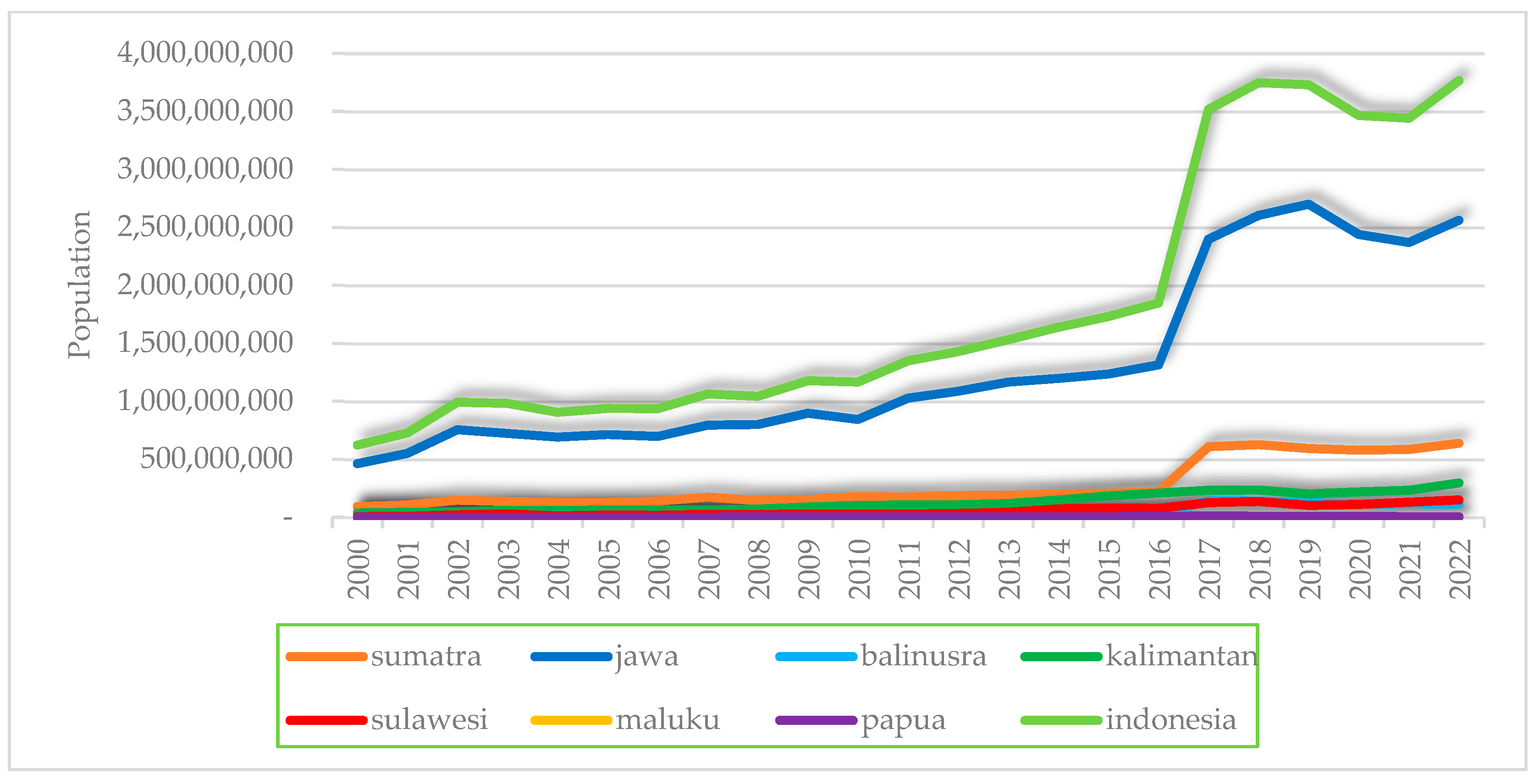
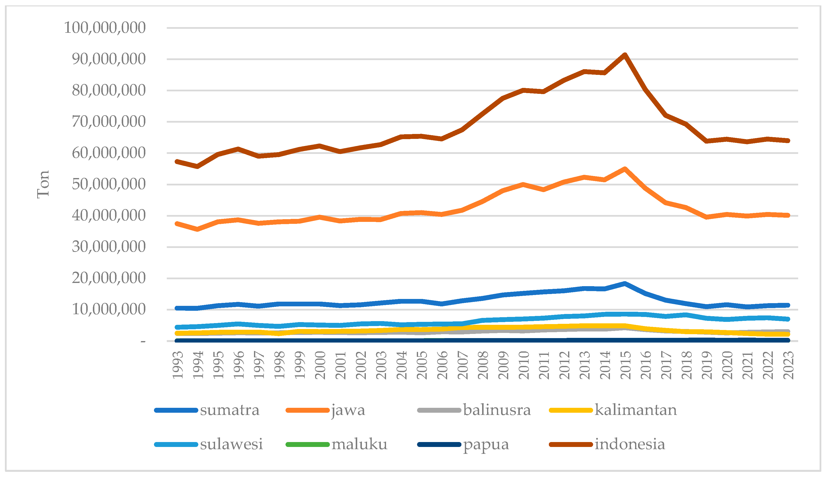
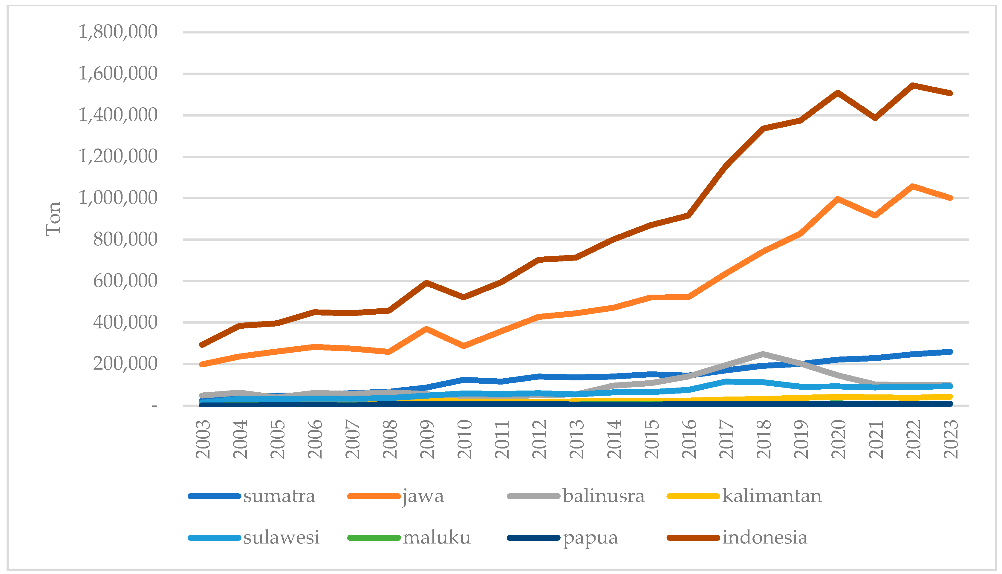
The dataset comprises monthly rural producer price data for the selected commodities from January 2009 to December 2022. The seven regions, Java, Sumatra, Kalimantan, Sulawesi, Bali–Nusa Tenggara, Maluku, and Papua, were chosen to reflect Indonesia’s major island groups, data availability, and agricultural diversity. Java serves as the reference region due to its role as the primary production and distribution hub, accounting for over 50% of national output for several key commodities (Shively & Thapa, 2017) and exerting a strong influence on inter-regional price movements. Production graphs by island for each commodity are provided in Appendix A, Figure A1, Figure A2, Figure A3, Figure A4, Figure A5 and Figure A6.

Before estimation, we tested all price series for stationarity using the Augmented Dickey–Fuller (ADF) and Phillips–Perron (PP) unit root tests, both including an intercept and a linear time trend to allow for deterministic components in the level series (Appendix A,

Table A1. Unit root test for monthly producer prices (2009–2022).

Commodity	ADF Test (Level)	ADF Test (1st Diff.)	PP Test (Level)	PP Test (1st Diff.)	Stationarity Conclusion
Rice	0.9596	0.0000 ***	0.9872	0.0000 ***	I(1)—use first differences
Chili	0.0000 ***	0.0000 ***	0.0119 **	0.0000 ***	I(1)—use first differences
Cayenne	0.0000 ***	0.0000 ***	0.0000 ***	0.0000 ***	I(1)—use first differences
Shallots	0.0016 ***	0.0001 ***	0.0053 ***	0.0000 ***	I(1)—use first differences
Eggs	0.4072	0.0000 ***	0.0434 **	0.0000 ***	I(1)—use first differences
Chicken	0.0508 *	0.0000 ***	0.0414 **	0.0000 ***	I(1)—use first differences

Notes: Tests include intercept and trend. p-values reported: *** Significant at 1% level, ** Significant at 5% level, * Significant at 10% level. All series are integrated of order one, I(1), and modeled in first differences for GARCH-type analysis. Although unit root tests indicate that some price series (e.g., chili and cayenne) are stationary in levels, while others (e.g., rice, eggs, chicken) are non-stationary, we consistently transform all variables into first differences prior to estimation. This decision is based on both statistical and methodological considerations. First, GARCH-type models—including DCC-GARCH—require input series to be covariance-stationary to ensure reliable estimates of conditional variance and correlation. Using first differences avoids the risk of spurious volatility persistence that can arise when working with borderline non-stationary series (e.g., p-values near 0.05). Second, consistent transformation across variables facilitates comparability and model stability, particularly in multivariate frameworks involving dynamic correlation structures.

). While some series are stationary in levels, all are stationary in first differences. Accordingly, we model conditional variance using first-differenced (stationary) series. In line with standard GARCH modeling practices (Engle, 2002; Enders, 2014; Brooks, 2019), no deterministic trend term is included in the DCC-GARCH specification because differencing removes any trend components, ensuring model parsimony and avoiding spurious volatility persistence.

To capture time-varying volatility in individual price series, we estimate Autoregressive Conditional Heteroskedasticity (ARCH) models (Engle, 1982) and their generalized form, GARCH models (Bollerslev, 1986). These models are widely used in commodity market research to account for volatility clustering, where current variance is affected by past shocks and previous volatility levels. While ARCH and GARCH models describe volatility patterns for single series, understanding spatial linkages requires a multivariate framework.

For this purpose, we apply the Dynamic Conditional Correlation GARCH (DCC-GARCH) model developed by Engle (2002), which captures both non-constant variance (heteroskedasticity) and evolving correlations among multiple price series. This framework is well-suited to track how volatility co-movements change over time and across markets, especially during periods of market dislocation, seasonal disruptions, or regional policy shocks. Previous applications in commodity markets, such as Got et al. (2013) on Ukrainian wheat and Bloznelis (2016) on segmented salmon markets, demonstrate the model’s ability to detect changing market integration and differentiated volatility behaviour across sub-markets, an insight highly relevant to Indonesia’s archipelagic economy.

The mean equation of the DCC-GARCH model is defined as:

$$H_{it}={\alpha }_{i0}+\sum _{j=1}^J{\alpha }_{ij}{H}_{it-1}+{\epsilon }_t$$

where $H_{it}$ is the price vector for commodity i in rural market j at time t, and ${\epsilon }_t$ is the error term vector.

The conditional variance-covariance matrix of the error term $\left({\epsilon }_t\right)$ is given by:

$$P=D_t{R_{t}D}_t$$

Here, $D_t$ is a diagonal matrix of time-varying standard deviations $\left({\sigma }_{it}^2\right)$, with each variance element modeled by a univariate GARCH process:

$${\sigma }_t^2=a_0+\sum _l^m{\alpha }_l{\mu }_{t-l}^2+\sum _k^s{\beta }_k{\sigma }_{t-j}^2$$

In the simplified GARCH (1, 1) form:

$${\mathsf{\sigma }}_{\mathrm{t}}^2={\mathrm{a}}_0+{\mathsf{\alpha }}_{\mathrm{l}}{\mathsf{\mu }}_{\mathrm{t}-\mathrm{l}}^2+{\mathsf{\beta }}_{\mathrm{k}}{\mathsf{\sigma }}_{\mathrm{t}-\mathrm{j}}^2$$

where ${\sigma }_t^2$ denotes the conditional variance of the conditional mean equation, ${\mu }_t^2$ denotes the squared error term of the conditional mean equation, and alphas and betas are summarized as theta ($\theta$). Then, GARCH (a, b) is

$$\theta =\sum _l^a{\alpha }_l+\sum _k^b{\beta }_k$$

or in a typical GARCH (1, 1), $\theta ={\alpha }_1+{\beta }_1$.

The sum of the ARCH and GARCH coefficients (α and β), denoted as $\theta$, represents the volatility persistence parameter. A $\theta$ close to 1 implies that the conditional variance takes a longer time to return to its long-term mean or volatility shocks decay slowly. If the value of $\theta$ > 1, then it suggests an explosive volatility, while $\theta$ = 1 means no tendency to revert or volatility does not revert to the long run mean. The speed of conditional mean returns to the value of its long-term mean is measured by calculating the time required for the conditional mean to fill half of the value gap of the long-term mean. The half-life of a shock or the number of periods required for volatility to revert halfway to its mean is calculated as:

$$M={\displaystyle \frac{ln\left(0.5\right)}{ln\left(\theta \right)}}$$

For example, if $\theta$ = 0.7, then the volatility gap will revert halfway to its mean in approximately 1.94 periods. While $\theta$ = 1 indicates the half-life becomes infinite, suggesting that volatility does not revert to the mean or there is no mean reversion (Bloznelis, 2016).

The dynamic correlation matrix $D_t$ is defined as:

$${\mathrm{D}}_{\mathrm{t}}={\left(\mathrm{d}\mathrm{i}\mathrm{a}\mathrm{g}\left({\mathrm{S}}_{\mathrm{t}}\right)\right)}^{-{\displaystyle \frac{1}{2}}}{{\overline{\mathrm{S}}}_{\mathrm{t}}\left(\mathrm{d}\mathrm{i}\mathrm{a}\mathrm{g}\left({\mathrm{S}}_{\mathrm{t}}\right)\right)}^{-{\displaystyle \frac{1}{2}}}$$

where

$${\mathrm{S}}_{\mathrm{t}}=\left\{{\mathrm{q}}_{\mathrm{i}\mathrm{j},\mathrm{t}}\right\}=\left(1-\mathsf{\alpha }-\mathsf{\beta }\right){\overline{\mathrm{S}}}_{\mathrm{t}}+\mathsf{\beta }{\mathrm{S}}_{\mathrm{t}-1}+\mathsf{\alpha }\left({\mathsf{\mu }}_{\mathrm{t}-1}{\mathsf{\mu }}_{\mathrm{t}-1}\right)$$

This formulation focuses on calculating the time-varying conditional correlations $C_t$:

$${\mathsf{\tau }}_{\mathrm{i}\mathrm{j},\mathrm{t}}={\displaystyle \frac{{\mathrm{q}}_{\mathrm{i}\mathrm{j},\mathrm{t}}}{\sqrt{{\mathrm{q}}_{\mathrm{i}\mathrm{i},\mathrm{t}}}\sqrt{{\mathrm{q}}_{\mathrm{j}\mathrm{j},\mathrm{t}}}}}$$

Here, $S_t=\left\{q_{ij,t}\right\}$ is the time-varying covariance matrix of standardized residuals from the mean equation. ${\overline{S}}_t$ represents its unconditional counterpart. Parameters α and β are non-negative and must satisfy α + β < 1 as adjustment terms. The parameter α reflects the immediate response of volatility to new information (shock effects), while β represents the influence of previous periods’ volatility (Got et al., 2013; Bloznelis, 2016). In this study, the term long-run conditional correlation refers to the average DCC-GARCH correlation over the 2009–2022 sample period. Values above 0.90 indicate strong and persistent co-movements in volatility between Java and other regions (or high market integration). This definition ensures that the interpretation of correlation magnitudes in Section 5 is consistent with the econometric measure applied.

A significant ARCH term indicates that recent shocks to log returns have a measurable influence on current price volatility. The size of the ARCH coefficient reflects the strength of that impact. A significant GARCH term indicates the persistence in volatility, which means that current volatility is linked to previous volatility levels. The sum of the ARCH and GARCH coefficients ($\theta$) quantifies overall volatility persistence. When the $\theta$ value is near 1, the shock effects tend to last longer (Verbeek, 2008).

The half-life (M) provides a useful interpretation of how quickly the volatility returns to revert halfway to its mean level. Markets with high ARCH and GARCH coefficients and long half-lives are considered to be much volatile and risky. Spatial differences in these magnitudes and significance reveal regional differences in volatility exposure across rural markets. Finally, the DCC model also assesses the extent of correlation in volatility across correlated markets over time. Higher conditional correlations indicate a stronger connection or closer price co-movement between market pairs, while lower or negative correlations indicate more localized volatility dynamics. The insights help reveal spatial structures in food price behaviour and inform targeted market interventions.

While this study employs ARCH, GARCH, and DCC-GARCH models to capture inter-regional volatility dynamics, we acknowledge that the exclusion of exogenous explanatory variables, such as weather shocks (e.g., El Niño), global food prices, exchange rates, or trade interventions, limits the model’s explanatory scope. However, this decision was grounded in two key considerations.

First, the commodities selected in this study-such as shallots, chili, and cayenne-are predominantly domestically produced and consumed, with minimal exposure to global markets or external price transmission mechanisms. Their price behavior is shaped primarily by local production cycles, transportation bottlenecks, and intra-island distribution rather than international trade flows or currency fluctuations (Qin & Zhang, 2016; Nazlioglu et al., 2013).

Second, many relevant external variables are either unavailable at a monthly frequency or lack sufficient spatial resolution for subnational modeling over the full 2009–2022 period. For instance, ENSO (El Niño–Southern Oscillation) indices are constructed at the global scale and cannot be directly mapped to region-specific agricultural outcomes across Indonesia’s diverse climate zones. Similarly, policy instruments such as subsidies or trade restrictions are enacted intermittently and are not consistently recorded at the provincial level. Including such coarse or irregular data may introduce measurement noise and obscure the true volatility dynamics under investigation (FAO, 2020).

Despite these limitations, we recognize the potential of including exogenous regressors in future extensions of the model, particularly for commodities more exposed to international markets, such as rice and beef. As high-resolution weather and trade datasets become increasingly available, structural volatility models could be developed to disentangle external shocks from internal drivers and enrich our understanding of spatial price risks in Indonesia.

5. Results

5.1. Food Producer Price Volatility Analysis

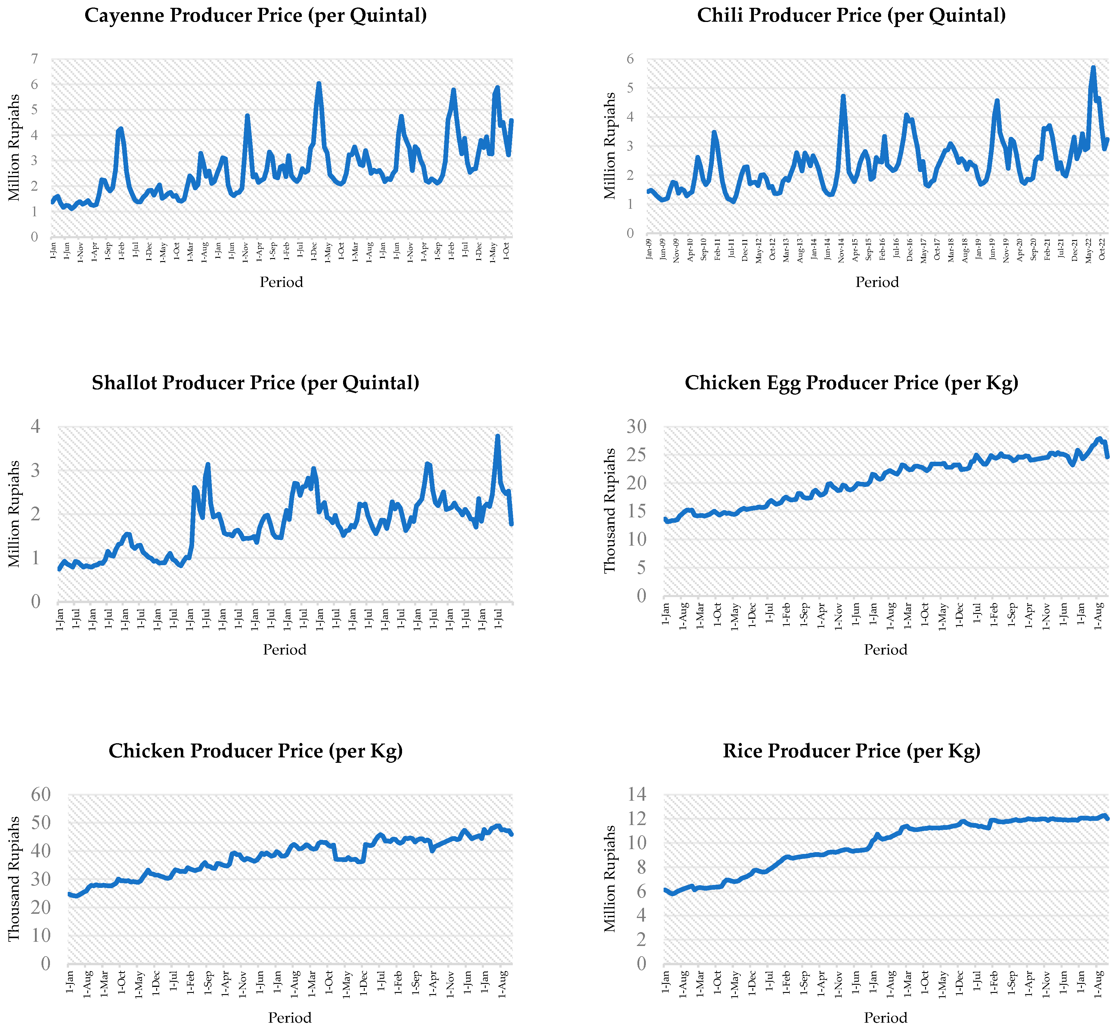
This study draws on monthly producer price data for six major food commodities in Indonesia: chicken, egg, chili, cayenne, shallot, and rice. The dataset spans 14 years, from January 2009 to December 2022, providing 168 monthly observations for each commodity. These data were obtained from the Village Producer Price Survey conducted by Statistics Indonesia (BPS). Figure 1 illustrates the time series for each commodity, highlighting the trends and fluctuations in producer prices over time.

The volatility behavior of these food commodity prices provides critical insight into market efficiency, supply chain robustness, and the vulnerability of consumers and producers to shocks. Using a GARCH modeling framework, the results reveal stark differences in the nature and persistence of volatility across the six staples (

Table 1. Food producer price volatility analysis.

Commodity	Arch Value	Garch Value	Volatility
Chili	-	0.99900	0.999034
Shallot	0.3507	0.52392	0.874487
Chicken	-	0.99890	0.998921
Rice	-	0.99900	0.999091
Egg	-	0.99900	0.999001
Cayenne	-	0.99900	0.999058

Note: Estimates are from univariate GARCH (1, 1) models for Java’s producer prices. “Volatility” is the sum (α + β), indicating persistence. A “-” indicates an ARCH term not included or not significant. Data source: BPS Village Producer Price Survey (rural Indonesia, all provinces). All GARCH coefficients are significant at the 1% level.

). Nearly all commodities exhibit volatility persistence parameters (α + β) close to 1, indicating that rural producer prices are highly volatile and shocks have long-lasting effects. For instance, chili, chicken, rice, egg, and cayenne all have α + β values exceeding 0.99, implying extremely unstable prices prone to large fluctuations. Such high volatility is often driven by inefficiencies in supply chains, including poor infrastructure, logistical challenges, and delays in transportation and distribution. Adverse weather conditions (droughts, floods, storms) also play a crucial role by disrupting supply and causing sharp price spikes (Qin & Zhang, 2016; Nazlioglu et al., 2013). In addition, speculative trading based on expectations of future shortages or gluts can exacerbate price swings, as traders might buy or sell large quantities in anticipation of price movements.

Table 1 confirms that volatility persistence is near-unit for most commodities. In practical terms, this means markets experience volatility clustering: periods of calm are followed by prolonged periods of high volatility, as shocks echo through time rather than dissipating quickly. Weak storage systems, limited market integration, and slow transportation can amplify these patterns. Under such conditions, even minor disruptions, such as a fuel price hike, a brief export ban, or a local harvest shortfall, can trigger disproportionate and enduring price surges (Gilbert & Morgan, 2010; FAO et al., 2011). These volatility episodes pose serious risks, undermining food security and complicating inflation control.

Visually, price trajectories for cayenne, shallots, and chili display sharp seasonal peaks and pronounced fluctuations, consistent with their perishable nature and exposure to weather and supply chain disruptions (Rahmawati et al., 2019; Haile et al., 2019). By contrast, staples such as rice and eggs exhibit relatively smoother price paths over time. The visual trends do not contradict the statistical findings in Table 1: whereas Figure 1 presents raw price levels, Table 1 summarizes volatility metrics from univariate ARCH/GARCH models. The ARCH coefficients capture short-term jumps in volatility from recent shocks, while the GARCH coefficients reflect the persistence or “memory” of volatility over time, patterns not always apparent from raw price series (Engle, 1982; Bollerslev, 1986). For example, rice and eggs, despite modest day-to-day price movements, register high and statistically significant GARCH coefficients, suggesting that their volatility is persistent and systemic rather than episodic. This indicates that even in the absence of dramatic price spikes, these commodities carry substantial long-term uncertainty (Haile et al., 2019). On the other hand, cayenne and shallots show both visible price spikes and elevated ARCH/GARCH effects, underscoring their role as the most unstable items in the rural food system (Rahmawati et al., 2019).

Table 1 shows that for five of the six commodities, the GARCH term (β) is very close to 1 and dominates the volatility dynamics. In these cases, once a shock hits, its influence on volatility decays extremely slowly. For shallots, however, the sum (α + β) is about 0.8745, which, while still high, is noticeably lower than the 0.999 seen for the others. Shallots have a significant ARCH term (α ≈ 0.35) and a moderate GARCH term (β ≈ 0.524), indicating that shallot price volatility is driven more by short-term shocks than by prolonged volatility clustering. In other words, the shallot market appears somewhat more responsive in the short run (e.g., prices jump with a bad harvest) but does not sustain volatility as long as the other commodities. If shallot cultivation and distribution are relatively more resilient to disruptions (for instance, due to quicker harvest cycles or better local storage/trade networks), prices would exhibit less persistence in volatility. This suggests that shallot price dynamics are dominated by recent shocks rather than long memory of past volatility, perhaps due to faster supply responses or a more competitive, responsive market structure. Indeed, the volatility persistence for shallots (0.8745) is significantly lower than the nearly unitary values observed for the other commodities. This finding aligns with the idea that certain horticultural crops with more efficient distribution channels or a larger number of market participants exhibit lower volatility persistence.

High price volatility has serious implications for both consumers and producers. For consumers, especially low-income households, volatile food prices make budgeting difficult and can threaten food security as spikes force reductions in food quantity or quality. For producers, high volatility means greater uncertainty in income, making it challenging to plan investments or manage resources. Farmers might hesitate to invest in expanding production if prices swing unpredictably, and sudden price drops can devastate their earnings. Policymakers, therefore, face pressure to stabilize food prices by addressing the underlying causes of volatility. This could involve investing in infrastructure to improve supply chain efficiency (e.g., better rural roads, cold storage facilities), implementing measures to mitigate the impact of climatic variability (such as irrigation and drought-resistant seeds), and regulating speculative activities in commodity markets to prevent excessive price swings.

From a policy perspective, the divergence in volatility patterns across commodities implies that a one-size-fits-all approach to market stabilization would be inefficient. For commodities with extremely high GARCH persistence (almost unit-root behavior), interventions should prioritize long-term infrastructure and capacity investments. Examples include cold storage facilities, rural transportation improvements, and crop insurance schemes to buffer against climate-induced supply shocks. These measures can help mitigate the supply-side constraints that often prolong volatility episodes. Conversely, for commodities like shallots that exhibit more short-term volatility, targeted short-term interventions may be more effective. This could involve improving market information systems (so farmers and traders can respond quickly to gluts or shortages), providing temporary subsidies or purchasing programs during harvest gluts to prevent price crashes, and strengthening demand-side measures such as promoting processing or storage for surplus produce. Moreover, the near-unit-root behavior of volatility in staple commodities (rice, chicken, eggs) underscores the importance of building early warning systems and adaptive policy frameworks. Rapid response mechanisms, such as timely release of government buffer stocks, import/export adjustments, or emergency transport logistics, can help prevent localized price shocks from ballooning into broader crises, particularly for low-income households that spend a large share of their income on food.

5.2. Volatility Spillover Effect of Food Producer Price Analysis

We now turn to the spatial volatility spillovers across regions. The DCC-GARCH model allows us to quantify how volatility in Java’s producer prices co-moves with volatility in other regions. In what follows, we present the results for each major island group vis-à-vis Java, including a summary of production shares (to contextualize market size and dependence) and the estimated dynamic conditional correlations.

Java vs. Sumatra: 

Table 2. DCC-GARCH fit of Java and Sumatra.

Commodity	Average Production per Month of Java		Average Production per Month of Sumatra		Prob [Joint] dcca1	Prob [Joint] dccb1
	Ton	%	Ton	%
Chili	85,770	41.23	42,549	20.45	0.000000	0.838297
Shallot	142,964	65.22	10,720	4.89	0.000000	0.663324
Chicken	173,186,428	68.48	27,494,617	10.87	0.000000	0.906323
Rice	4,630,789	50.84	1,373,109	15.07	0.000000	0.920540
Egg	248,119	65.80	54,171	14.37	0.000000	0.944533
Cayenne	88,638	57.08	13,577	8.74	0.000000	0.922127

Note: “dcca1” is the p-value for the joint significance of short-run volatility correlation (0: no short-run correlation), and “dccb1” is the p-value for long-run correlation between Java and Sumatra. All values are from the DCC-GARCH model output. Java production percentages are the share of national production; Sumatra percentages are the share of national production.

summarizes the average monthly production of the six commodities in Java and Sumatra, as well as the joint test probabilities for the DCC-GARCH correlations (dcca1 for short-run, dccb1 for long-run). The comparison of production highlights Java’s dominance: Java produces over 65% of Indonesia’s chicken and eggs, and more than 50% of national rice and shallot output. Sumatra’s contributions are much lower; only in rice does Sumatra exceed 15% of national production. This concentration suggests a pronounced asymmetry in production that could influence price dynamics and volatility spillovers, given Sumatra’s reliance on inflows from Java for many commodities.

The DCC-GARCH estimates show statistically significant volatility co-movement between Java and Sumatra for all six commodities, as indicated by the dcca1 joint p-values, which are essentially zero for every commodity (Table 2). In other words, we decisively reject the null hypothesis that price volatilities in Java and Sumatra evolve independently. Volatility shocks in one region tend to be mirrored in the other, a clear sign of inter-regional price integration (Barrett & Li, 2002; Serra & Goodwin, 2003).

However, the strength of these linkages varies by commodity, especially in the long run. The dccb1 probabilities in Table 2 point to heterogeneous correlation magnitudes. Commodities like cayenne, rice, and chicken show very high long-run correlation (dccb1 p-values around 0.90 or above), implying tightly synchronized volatility movements between Java and Sumatra. This is plausible given Java’s role as a supply hub and Sumatra’s dependence on inter-island trade flows for staple and high-demand items. In contrast, shallots and chili have lower (though still significant) long-run correlations (around 0.66 and 0.84, respectively), suggesting relatively weaker integration for these commodities. This may reflect the more localized nature of shallot and chili markets, both in production (certain areas specialize in these spices) and in consumption preferences, or logistical frictions in transporting perishable produce over long distances. Differing harvest calendars, limited cold storage, and region-specific varieties could also dampen the volatility linkage for these crops.

Overall, the Java–Sumatra results underscore two insights. First, Java functions as a central node in Indonesia’s food supply network: its production dominance translates into volatility dominance, meaning price volatility originating in Java has a broad national reach. Second, the strong dynamic volatility correlations between Java and Sumatra indicate a high degree of market integration between the two largest island economies. Any major disruption in Java, be it a natural disaster, a transportation bottleneck, or a policy change, can induce volatility spillovers in Sumatra. This interdependence has important policy implications. It highlights the need for regional buffer mechanisms (such as decentralized food storage facilities or redundant logistics routes) to cushion Sumatra against volatility emanating from Java. For example, maintaining buffer stocks in Sumatra or improving port and shipping resilience could help moderate transmitted shocks, especially for highly volatile and crucial commodities like chili, chicken, and rice.

Java vs. Bali–Nusa Tenggara: Java and the combined region of Bali–Nusa Tenggara present a different dynamic (

Table 3. DCC-GARCH fit of Java and Bali–Nusa Tenggara.

Commodity	Average Production per Month of Java		Average Production per Month of Bali Nusa Tenggara		Prob [Joint] dcca1	Prob [Joint] dccb1
	Ton	%	Ton	%
Chili	85,770	41.23	66,548	31.99	0.442270	0.899705
Shallot	142,964	65.22	50,696	23.13	0.000000	0.870221
Chicken	173,186,428	68.48	14,756,070	5.83	0.040045	0.951907
Rice	4,630,789	50.84	990,057	10.87	0.000000	0.922844
Egg	248,119	65.80	30,523	8.09	0.045886	0.367637
Cayenne	88,638	57.08	31,394	20.22	0.000000	0.914136

). Java consistently dominates national production for all commodities, providing over 65% of eggs and chicken and more than 50% of rice, shallots, and cayenne. Bali–Nusa Tenggara, in contrast, contributes relatively modest shares; its highest contributions are approximately 31.9% for chili and 23.1% for shallots, while for other commodities it supplies under 15% of national output (BPS, 2022). This skewed production structure reinforces Java’s role as the core food supply hub and implies that Bali–Nusa Tenggara relies substantially on inflows from Java for many staples.

Despite this asymmetry, the DCC-GARCH results reveal notable volatility correlations, but with some variation across commodities. The short-run co-movement (dcca1) is statistically significant for most commodities, indicating that volatility shocks in Java do transmit to Bali–Nusa Tenggara in the immediate term. In particular, we find highly significant short-run correlations for shallot and cayenne (p = 0.000000), and significant (at 5% level) for chicken (p ≈ 0.044) and egg (p ≈ 0.046). Chili is an exception in the short run, with a dcca1 p-value (around 0.442) that is not significant, suggesting that short-term volatility in chili prices may not be strongly synchronized between Java and Bali–Nusa Tenggara. This could be due to Bali–Nusa Tenggara’s partial self-sufficiency in chili or short-term trade frictions (perhaps chili supply to Bali comes from closer islands or is limited by inter-island transport capacities in the short run).

In the long run, the dccb1 results indicate strong integration for certain commodities. For example, the long-run volatility correlation for shallots between Java and Bali–Nusa is extremely high (dccb1 p ≈ 0.97), implying that over time their volatility patterns become almost unified. Chicken, rice, and egg also show high long-run correlations (roughly 0.90 or above), consistent with Bali–Nusa Tenggara’s heavy dependence on Java for these staples. On the other hand, chili and cayenne exhibit more moderate long-run correlations with Java (dccb1 values in the 0.64–0.74 range). This suggests that while Bali–Nusa Tenggara is integrated with Java’s markets in general, certain spice commodities still retain some independent volatility behavior in the long run, potentially due to local consumer preferences, smaller trade volumes, or isolated production pockets within Bali–Nusa that buffer long-term volatility.

In summary, Java and Bali–Nusa Tenggara have intermediate integration with some commodity-specific nuances. The existence of significant volatility co-movement for most commodities confirms that Java’s market shocks reverberate in Bali–Nusa Tenggara. However, the variation for chili and cayenne indicates selective integration, possibly influenced by fragmented transport links or commodity-specific trade patterns. Policy-wise, this points to the value of infrastructure development and market harmonization in the Bali–Nusa Tenggara region. Strengthening ferry links and roads, improving storage for perishable goods, and aligning market information systems could enhance integration where needed and reduce regional price volatility disparities. For example, if chili volatility is less connected, efforts to integrate Bali–Nusa Tenggara’s chili market with Java (through better logistics or encouraging inter-island trade) could help stabilize prices on both ends.

Java vs. Kalimantan: 

Table 4. DCC-GARCH fit of Java and Kalimantan.

Commodity	Average Production per Month of Java		Average Production per Month of Kalimantan		Prob [Joint] dcca1	Prob [Joint] dccb1
	Ton	%	Ton	%
Chili	85,770	41.23	3861	1.86	0.160307	0.485122
Shallot	142,964	65.22	179	0.08	0.000000	0.815836
Chicken	173,186,428	68.48	25,932,303	10.25	0.000000	0.956348
Rice	4,630,789	50.84	798,497	8.77	0.000000	0.942830
Egg	248,119	65.80	21,152	5.61	0.000000	0.913608
Cayenne	88,638	57.08	5739	3.70	0.000000	0.915844

presents the production and DCC-GARCH correlation results for Java and Kalimantan. Kalimantan represents a middle-ground case: it is neither as large a producer as Java nor as minor as regions like Maluku. It contributes moderately to national output in some items, about 10.25% for chicken and 8.77% for rice, but remains very small in others (less than 2% for chili and under 1% for shallots). This mix suggests that Kalimantan has some self-sufficiency in certain staples but is largely dependent on Java for others, especially horticultural products and perishables.

Kalimantan’s DCC-GARCH results show strong long-run volatility co-movements (dccb1) across nearly all commodities with Java. Specifically, chicken, rice, egg, and cayenne all have very high long-run correlation p-values (around 0.91–0.96), indicating that in the long term, volatility in those markets moves closely in tandem with Java. This suggests that Kalimantan’s food markets have become increasingly integrated with Java’s over time, likely due to inter-island trade flows, nationwide pricing policies, and the growing penetration of common distribution networks. For instance, staples and proteins like chicken and rice might be subject to national market forces (e.g., government rice operations, large poultry distributors) that link Kalimantan prices to conditions in Java.

In the short run, the picture is more nuanced. The short-run correlation (dcca1) for chili is not statistically significant (p ≈ 0.1603), implying that immediate volatility shocks in Java’s chili prices do not strongly affect Kalimantan’s chili market. This could be due to logistical delays (chili takes time to ship from Java to Kalimantan, so a shock today in Java might reach Kalimantan with a lag), perishability (spice prices in Kalimantan might spike due to local factors before Java’s influence kicks in), or generally weaker short-term market responsiveness for that commodity. In contrast, all the other commodities do show significant short-run co-movement: chicken, rice, egg, and cayenne each have dcca1 p-values of 0.000000, indicating rapid transmission of volatility from Java to Kalimantan for those goods. These products likely benefit from well-functioning trade channels and fast price signal transmission, perhaps because they are traded in high volumes year-round (chicken, rice, eggs) or because markets arbitrage quickly (as with nationally traded staples).

These findings suggest that Kalimantan is transitioning from a peripheral market to a semi-integrated regional hub, particularly for key proteins and staples. The region’s exposure to Java’s volatility is high in both the short and long run for most commodities, meaning Kalimantan’s consumers and traders feel the ripple effects of shocks in Java fairly quickly and persistently. The exception of chili highlights a commodity where Kalimantan might have a bit more insulation or delay. Policy strategies for Kalimantan, therefore, should aim to further upgrade intra-regional logistics and market linkages, especially to improve short-run integration for perishables like chili and shallots. Investments in cold storage, better inter-island shipping capacity, and local production incentives for these commodities could reduce delays and improve price stability. Additionally, implementing Java-Kalimantan coordinated price management systems (for instance, synchronized release of stockpiles or transport subsidies during price spikes) would be beneficial for commodities like chicken and rice, where co-movements are strongest and the stakes for food security are high.

More broadly, the Java-Kalimantan analysis reinforces a general pattern: volatility co-movement is not solely a function of a region’s production share. Infrastructure quality, trade connectivity, and supply chain integration play crucial roles. Kalimantan’s rice volatility, for example, co-moves strongly with Java’s despite Kalimantan producing less than 9% of the rice, underscoring that even regions with modest production can be highly integrated if distribution networks tightly link them to the core.

Java vs. Sulawesi: 

Table 5. DCC-GARCH fit of Java and Sulawesi.

Commodity	Average Production per Month of Java		Average Production per Month of Sulawesi		Prob [Joint] dcca1	Prob [Joint] dccb1
	Ton	%	Ton	%
Chili	85,770	41.23	5894	2.83	0.000000	0.583620
Shallot	142,964	65.22	13,515	6.17	0.000000	0.970617
Chicken	173,186,428	68.48	9,392,575	3.71	0.000000	0.915958
Rice	4,630,789	50.84	1,178,884	12.94	0.000000	0.866120
Egg	248,119	65.80	19,000	5.04	0.000000	0.835221
Cayenne	88,638	57.08	10,776	6.94	0.074316	0.643127

shows the results for Java and Sulawesi. Java continues to dwarf Sulawesi in production of most commodities, providing over 65% of the national chicken and egg supply and more than half of rice, shallots, and cayenne. Sulawesi’s contributions are modest, ranging from about 2.8% of national chili production to roughly 12.9% of rice (its highest share). This asymmetry is somewhat less extreme than in the Maluku or Papua cases, but it still positions Java as the dominant market that likely drives national price trends, with Sulawesi being a secondary player.

Despite Sulawesi’s lower production shares, the DCC-GARCH results indicate statistically significant short-run volatility co-movement for nearly all commodities. The dcca1 tests are essentially zero (highly significant) for chili, shallot, chicken, rice, and egg, implying that price volatility shocks in Java are transmitted quickly to Sulawesi for those items. This finding is consistent with spatial price transmission theory and previous evidence of inter-island price linkages in archipelagic economies: even if Sulawesi produces only a small fraction of, say, Java’s rice, any volatility in Java’s large market can rapidly spill over via trade and expectations into Sulawesi’s prices.

However, cayenne is a notable outlier. The short-run correlation for cayenne (dcca1 p ≈ 0.0743) is above conventional significance thresholds, indicating weak or no immediate volatility co-movement between Java and Sulawesi for this commodity. This parallels what we saw with chili in Kalimantan (and to a lesser extent chili in Bali–Nusa Tenggara): certain spices or perishable commodities do not show fast volatility transmission, likely due to localized market conditions or less integrated trade flows for those specific crops. For cayenne, it could be that Sulawesi has distinct production cycles or varieties, or that the inter-island trade in cayenne is limited/slow, leading to a dampened immediate response to Java’s price shocks.

In terms of long-run volatility integration, the dccb1 results reveal high and significant correlations for most commodities. Shallot stands out with an extremely high long-run correlation (0.9706), meaning Sulawesi’s shallot market volatility eventually moves almost in lockstep with Java’s. Rice, egg, and chicken also have quite high long-run correlations (0.86–0.92 range), suggesting that over time, volatility shocks in Java persist and become synchronized with price movements in Sulawesi, despite the production gap. The mechanism here is likely through wholesale and distribution channels: if prices in Java stay high or volatile due to a prolonged shock, suppliers and traders in Sulawesi adjust their prices in response (and vice versa to some extent), leading to converging volatility trends.

Interestingly, chili and cayenne show only moderate long-run correlations (around 0.58 and 0.64, respectively). This could imply that Sulawesi retains a bit more independent price formation for these volatile perishables. Perhaps local demand and supply factors (like the extent of chili pepper cultivation in Sulawesi’s uplands, or consumption preferences) cause some decoupling in volatility from Java over the long run. It echoes prior research that perishables can be regionally segmented due to spoilage risks, higher transport costs relative to value, and asynchronous harvests (Nazlioglu et al., 2013).

From a policy standpoint, the Sulawesi case emphasizes that the island is not insulated from Java’s volatility shocks, even though it contributes less to overall production. Sulawesi experiences both quick and enduring volatility spillovers for staples and poultry. Therefore, reinforcing intra-regional resilience is important. This could involve building more localized storage systems (to buffer short-term supply shocks), providing production incentives to increase Sulawesi’s self-sufficiency in key foods (reducing over-reliance on Java), and granting greater logistic autonomy (e.g., dedicated shipping routes or emergency stock release for Eastern Indonesia) to manage volatility. For commodities with especially high DCC values (rice, eggs, chicken), the national food policy should explicitly coordinate inter-island supply chains and include price stabilization tools that account for Java’s centrality in driving price dynamics. In practice, this might mean synchronizing rice reserve releases between Java and Sulawesi during a shock, or ensuring telecommunication networks quickly disseminate price information to dampen panic and allow arbitrage.

Java vs. Maluku: Moving to one of the smallest contributors,

Table 6. DCC-GARCH fit of Java and Maluku.

Commodity	Average Production per Month of Java		Average Production per Month of Maluku		Prob [Joint] dcca1	Prob [Joint] dccb1
	Ton	%	Ton	%
Chili	85,770	41.23	1493	0.72	0.000000	0.341564
Shallot	142,964	65.22	591	0.27	0.000000	0.910704
Chicken	173,186,428	68.48	192,732	0.08	0.000000	0.919678
Rice	4,630,789	50.84	60,443	0.66	0.000000	0.902844
Egg	248,119	65.80	509	0.13	0.000000	0.725665
Cayenne	88,638	57.08	2082	1.34	0.000000	0.524811

details Java versus Maluku. Java’s dominance is extreme here: Java produces over 65% of several commodities, whereas Maluku produces well under 1% of national output for most items (e.g., ~0.7% of chili, 0.3% of shallots, 0.08% of chicken). Maluku’s highest share in this list is not even 1% (cayenne might be slightly higher, but still negligible). This stark imbalance illustrates Maluku’s deep structural dependence on Java and other islands for food supply.

Even with Maluku’s minimal production, the DCC-GARCH results show statistically significant short-run and long-run volatility co-movements for nearly all commodities. All dcca1 p-values are essentially zero, which means volatility shocks in Java do have an immediate and statistically significant impact on Maluku’s price volatility for those commodities. This finding is striking: despite Maluku producing almost none of these products, its markets are not isolated. It implies that Maluku’s prices respond to news or supply changes in Java very quickly, likely because Maluku imports a large portion of its food, so local prices adjust as soon as Jakarta or Java prices move (plus perhaps speculative stockpiling behavior by traders anticipating changes).

The long-run correlations (dccb1) are also high for most items. For instance, shallots, chicken, and rice show dccb1 values around 0.90 or above, indicating very strong persistent co-movement in volatility with Java. This is intuitive; Maluku’s prices in the long term largely reflect the conditions in the markets of Java (and possibly Sulawesi/Papua if they serve as intermediate hubs), given Maluku’s negligible local supply. The chili case is a bit different: the long-run correlation for chili is lower (around 0.34), which is surprisingly low compared to others. It might be an anomaly or possibly indicates that Maluku does not rely on Java for chili to the same extent (maybe obtaining it from Sulawesi or local gardens), thus having a somewhat independent volatility pattern. Alternatively, it could reflect limited data or an outlier issue. Nonetheless, all commodities have highly significant dcca1 (short-run) links, so even chili shows an immediate reaction, even if the sustained correlation is lower.

In essence, Maluku emerges as extremely dependent on Java: it is a price-taker region with volatility essentially imported from Java’s market. When Java sneezes, Maluku catches a cold, so to speak, in terms of price volatility. This condition justifies targeted interventions. The findings support policies such as establishing regional food buffer stocks in Maluku, subsidizing inter-island logistics to ensure consistent supply (so that small disruptions do not cause huge local price spikes), and even modest local production incentives for strategic commodities. For example, encouraging small-scale poultry or egg production in Maluku could provide a local buffer against volatility in those markets. Similarly, improving the shipping frequency and capacity between Maluku and Java (or Sulawesi) could reduce volatility by smoothing out supply delays.

Java vs. Papua: Finally, Java versus Papua represents the most extreme core-periphery relationship in our study. Papua is geographically distant, has an isolated and often undersupplied market, and produces less than 1% of the national supply for almost all commodities. Indeed, Papua’s highest contribution among these is about 1.98% for cayenne and just 0.24% for shallots (BPS, 2022). This vast gap confirms Papua’s role as a structurally dependent region in Indonesia’s food system, heavily reliant on shipments from Java and other islands.

The DCC-GARCH analysis (

Table 7. DCC-GARCH fit of Java and Papua.

Commodity	Average Production per Month of Java		Average Production per Month of Papua		Prob [Joint] dcca1	Prob [Joint] dccb1
	Ton	%	Ton	%
Chili	85,770	41.23	1917	0.92	0.000000	0.696082
Shallot	142,964	65.22	528	0.24	0.000000	0.929209
Chicken	173,186,428	68.48	1,941,866	0.77	0.051594	0.921354
Rice	4,630,789	50.84	76,847	0.84	0.000000	0.902844
Egg	248,119	65.80	3604	0.96	0.000000	0.859454
Cayenne	88,638	57.08	3081	1.98	0.000000	0.918608

) shows that short-run volatility co-movement between Java and Papua is significant for all commodities except one. The dcca1 tests are 0.000000 for five commodities (rice, chili, shallot, egg, cayenne), meaning Java’s volatility immediately transmits to Papua’s prices in those cases. The only exception is chicken, where the p-value is ~0.0516 (just above the 5% threshold) (BPS, 2022). This suggests that short-run volatility in chicken prices in Java nearly spills over to Papua (and likely does so in a slightly delayed or slightly weaker fashion), which is not surprising, as Papua imports most of its chicken and eggs from other regions, but local market frictions may slightly delay the impact of Java’s volatility in the very short run. Still, the near-significance indicates that even chicken is on the cusp of immediate integration.

The long-run correlations are very high across the board (Nazlioglu et al., 2013; Qin & Zhang, 2016). Essentially, Papua’s volatility correlations with Java are all strong in the long term, meaning Papua’s price volatility trends align closely with Java’s when viewed over longer periods. Even for chicken, which had a marginal short-run link, the long-run correlation becomes strong (Papua’s chicken prices eventually reflect Java’s volatility). This outcome underscores the central vulnerability of Papua’s food system: despite minimal local production, Papua’s markets experience volatility that is effectively imported from Java. Papua is a classic price-taker region; its food security is tightly coupled with Java’s market behavior.

This reality reflects Papua’s limited food sovereignty. Because it produces so little of what it consumes, any volatility in the prices at the sources (Java or Sulawesi) is passed through to Papua. There might be slight dampening or delays due to transport time (it takes time for goods to travel to Papua), but given the high costs and infrequent shipments, even small supply hiccups can cause big swings in local Papua prices.

Consequently, national food security policies must include tailored interventions for Papua. The analysis suggests several: (1) Establish regional price stabilization funds or buffer stocks specifically for remote provinces like Papua. This could help intervene in the market when volatility spikes (e.g., release rice stocks in Jayapura when prices jump unexpectedly). (2) Provide subsidized inter-island logistics for key perishable goods destined for Papua. If shipping operators are incentivized to maintain regular service (even at a loss) during bad times, Papua’s supply will be steadier, reducing volatility. (3) Incentivize local production through agronomic support, land development, and technology transfer. While Papua may never be self-sufficient in staples like rice, there may be potential to expand local output of certain vegetables, roots, or poultry to cushion against supply disruptions from Java. Even small increases in local supply or storage (e.g., small-scale silos or cold storage facilities) could dampen volatility. Finally, given how closely Papua’s fate is tied to Java’s markets, integrating Papua into national early warning systems is crucial. If price monitoring indicates a looming shortage in Java, Papua’s authorities need to prepare (perhaps by arranging emergency shipments or price controls) before the shock fully hits them. In short, Papua should be explicitly accounted for in any supply chain risk assessments, ensuring that measures are in place to protect this vulnerable region from the whiplash of Java’s volatility.

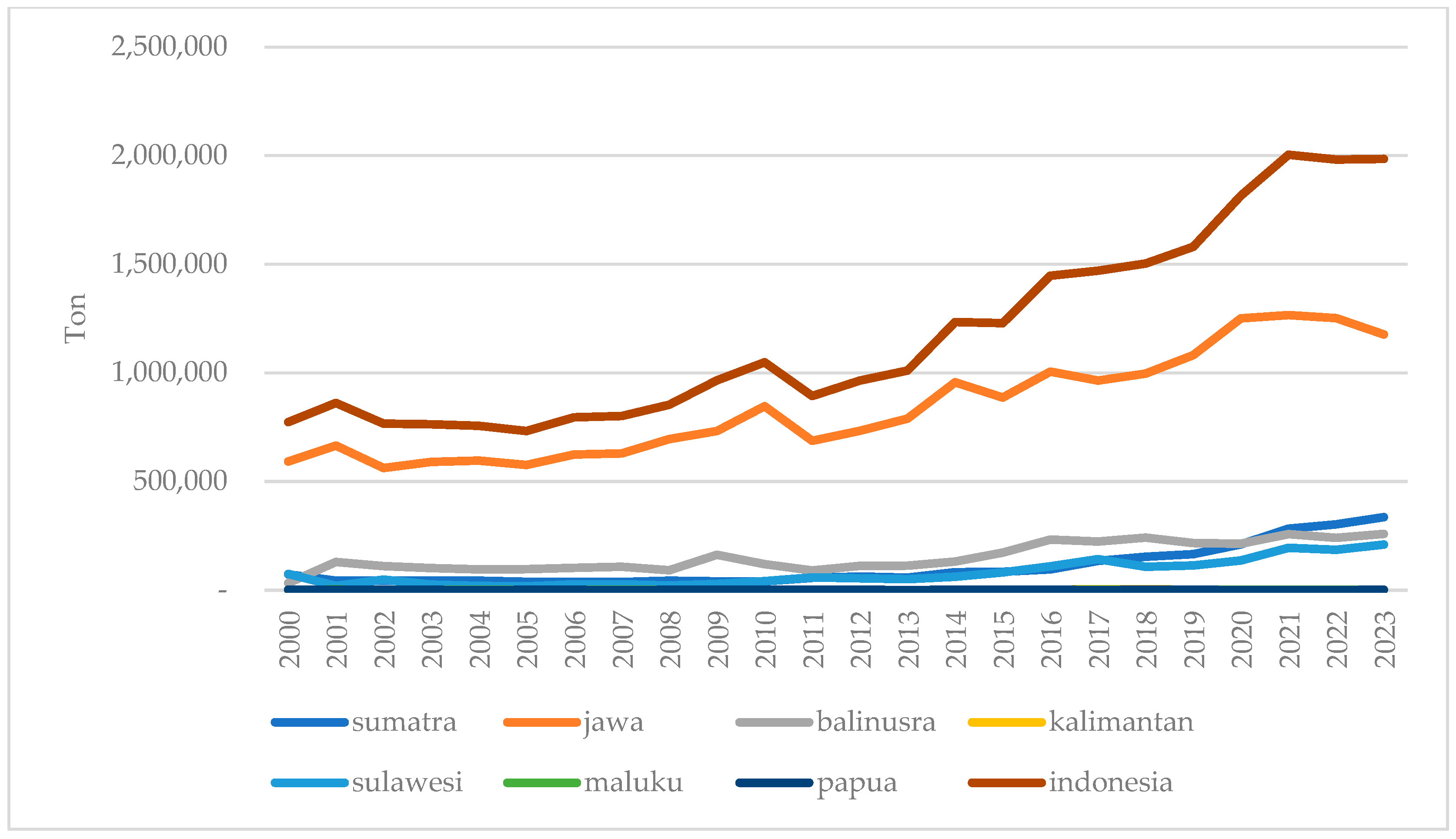
6. Discussion

The findings of this study underscore Java’s central role as both a production hub and a volatility transmitter in Indonesia’s food economy. The dynamic correlation analysis across Indonesia’s major regions, Java, Sumatra, Bali–Nusa Tenggara, Kalimantan, Sulawesi, Maluku, and Papua, reveals the spatial complexity of food price volatility transmission and consistently highlights Java’s pivotal influence in the national food system. We observe a clear pattern of volatility flowing outward from Java to other regions, albeit with varying magnitudes and durations across commodities and destinations (Barrett & Li, 2002). Despite wide heterogeneity in regional production capacities, all regions exhibit statistically significant short-run or long-run co-movements with Java’s food price volatility, though the intensity and persistence of these correlations vary by both region and commodity. In practical terms, this indicates a high degree of spatial price integration in volatility: upstream shocks in Java tend to propagate across the archipelago, making even distant markets responsive to Java’s price dynamics.

Java and Sumatra: These two populous islands show strong volatility linkages, especially for staple and high-demand commodities. Sumatra, while trailing Java in production, contributes meaningfully to national rice, egg, and chili supplies. The DCC-GARCH results indicate significant short-run and long-run volatility co-movement for most commodities, notably rice, chicken, and cayenne. The high long-run correlation values for chicken and cayenne (both above 0.90) reflect a well-integrated inter-island market (Rahmawati et al., 2019; Qin & Zhang, 2016). In essence, shocks in Java are rapidly transmitted to Sumatra and vice versa. This underscores the need for synchronized food security policies across the two islands, supported by robust trade infrastructure. For example, if a bad harvest drives up rice volatility in Java, Sumatra might release local reserves or expedite imports at the same time as Java to stabilize expectations on both islands.

Java and Bali–Nusa Tenggara: This pairing exhibits intermediate integration with some commodity-specific co-movement. Bali–Nusa Tenggara has moderate production contributions for a few commodities (e.g., chili, shallots) but depends on Java for many others (Rahmawati et al., 2019; Minten & Kyle, 2014). Short-run volatility co-movement is significant for most commodities, yet long-run correlations are more variable. For instance, cayenne, rice, and chicken have high long-run correlations (>0.9), whereas eggs and chili show weaker integration (Qin & Zhang, 2016). These variations suggest selective market integration, possibly influenced by fragmented transportation links or differences in commodity-specific supply chains. In this region, targeted improvements in infrastructure and market linkage could enhance integration. Strengthening inter-island transport (ferries, ports) and developing better storage facilities would likely reduce regional price disparities and improve the flow of goods and price signals.

Java and Kalimantan: The Java-Kalimantan relationship has a mixed profile. Kalimantan contributes moderately to national production in items like rice and chicken, and the results show strong long-run volatility co-movement for most commodities. However, short-run volatility synchronization is commodity-specific: for example, chili showed weaker short-run co-movement (insignificant in our tests) (Rahmawati et al., 2019; Roehner, 1996). In contrast, staples and livestock products had strong short-run linkages. This pattern implies that Kalimantan is largely integrated with Java’s market, but certain sectors (like chili) might still have buffers or delays, perhaps due to geography (long shipping routes) or local cultivation filling short-run gaps (Nazlioglu et al., 2013). Policy implication: Kalimantan could benefit from further integration for those lagging commodities. Improving supply chain reliability for perishables (e.g., investing in faster shipping or local greenhouse projects for chili) could bring even those markets into better alignment and stability.

Java and Sulawesi: We find high short-run dependence and emerging long-term linkages here. Sulawesi’s overall food production is modest compared to Java, but it plays a growing role in national rice and chicken output. The short-run volatility co-movement is significant for most commodities, indicating Sulawesi’s immediate responsiveness to Java’s market signals (Nazlioglu et al., 2013). Long-run linkages are more heterogeneous: shallots, rice, and chicken have strong long-run correlations, whereas chili and cayenne show weaker co-movement (Rahmawati et al., 2019; Roehner, 1996). This mixed pattern means Sulawesi is certainly vulnerable to Java’s volatility shocks, but some markets retain partial insulation, potentially due to localized consumer preferences or supply segmentation (e.g., Sulawesi might source cayenne from local farms for local consumption). To strengthen resilience, inter-island transport and information systems could be enhanced. Better ferry connections and real-time price information can tighten integration where beneficial, while also allowing Sulawesi to send surplus to Java when needed (which could mitigate volatility in Java too). Over time, as infrastructure improves (e.g., the new Trans-Sulawesi highways, better ports), we expect Sulawesi’s long-run integration with Java to increase, which is positive for arbitrage but also means local markets will need tools to cope with Java-driven volatility (Qin & Zhang, 2016).

Java and Maluku: This is an extreme dependency case. Maluku contributes less than 1.5% of the monthly national supply for all our commodities, reflecting a deep structural reliance on Java. Yet, the DCC-GARCH results show statistically significant short-run and long-run volatility co-movements for nearly all commodities (Barrett & Li, 2002; Rahmawati et al., 2019). Maluku is highly susceptible to imported price volatility despite its low production activity, consistent with the notion of peripheral or price-taker regions where volatility is externally determined. This finding justifies targeted interventions: establishing regional food buffers, providing logistics subsidies, and offering even modest local production incentives can be crucial. For example, Maluku might develop community-level grain warehouses to stabilize rice availability or provide subsidies for shipping basic foods from Java during lean seasons. Such strategies are in line with global recommendations on food price stabilization in remote regions (FAO et al., 2011; Qin & Zhang, 2016). The goal would be to partially uncouple Maluku’s volatility from Java’s by building some local shock absorbers, such as improved local storage or reduced transportation bottlenecks (Roehner, 1996).

Java and Papua: Papua’s situation is analogous to Maluku’s, perhaps even more pronounced. Papua produces less than 1% of the national supply for most commodities, yet still exhibits strong long-run volatility co-movement for almost all products and significant short-run linkages for all but chicken (Nazlioglu et al., 2013; Barrett & Li, 2002; BPS, 2022). This underscores the region’s price-taking role and deep exposure to Java-centric fluctuations. In such a context, the discussion points to boosting local food sovereignty as a long-term strategy. Encouraging localized production, even if limited to certain items like tubers, vegetables, or poultry, could reduce vulnerability. In the short run, Papua’s market would benefit from stabilization mechanisms tied directly to Java’s price dynamics, such as real-time price monitoring systems and coordinated subsidy allocation or emergency shipments when Java’s prices spike (FAO et al., 2011; Qin & Zhang, 2016). Essentially, national policy has to pay special attention to far-flung regions like Papua; otherwise, they bear the brunt of volatility without any local cushion, as high transport costs and long distances exacerbate exposure (Roehner, 1996).

Synthesizing across regions, this analysis reveals an asymmetrical but integrated food system where Java functions as the core volatility transmitter. Crucially, the strength of volatility co-movement (both short- and long-run) is not strictly proportional to a region’s production share. Even regions with minimal production (Maluku, Papua) are highly exposed to price volatility originating in Java. In contrast, semi-autonomous zones like Kalimantan and Sulawesi demonstrate more selective integration, hinting at potential leverage points for regional policy interventions. This suggests that market integration in Indonesia is driven less by co-production and more by distribution dependency. Peripheral markets often depend on Java-centric distribution networks; therefore, their prices are shaped less by local supply-demand dynamics and more by national-level fluctuations, often magnified by logistical delays or thin local markets.

Policy strategies should reflect this asymmetric dependence (Timmer, 2010). A dual resilience strategy is warranted. The first component is Java-centric stabilization measures that have system-wide implications. Given Java’s systemic role, policies aimed at stabilizing Java’s food prices (e.g., input subsidies for farmers, maintaining ample buffer stocks, using futures or options to hedge price risks) can yield spillover benefits across the entire country. For example, if volatility in Java’s rice market is tamed through effective buffer stock releases, consumers in outer islands indirectly benefit through more stable prices on imported rice from Java. Concretely, this strategy would involve maintaining and enhancing national food buffer stocks located in Java, strengthening price monitoring (perhaps through digital platforms that track prices in real time across regions), and enforcing preventive measures (like temporary price ceilings or anti-hoarding regulations) during extreme volatility episodes for core staples (FAO et al., 2011).

The second component must be region-specific interventions to complement the Java-centric approach. Peripheral regions should aim to reduce over-reliance on Java by investing in localized production capacities (especially for items like eggs, chicken, and chili that can be produced at smaller scales), and by subsidizing inter-island shipping to ensure these areas are not cut off during critical periods. For instance, remote regions like Papua, Maluku, and parts of Nusa Tenggara would benefit from government-supported shipping routes for food, which could operate even when private shippers find it unprofitable. Similarly, developing cold storage hubs in strategic locations (Sulawesi, Kalimantan, Maluku, Papua) would allow these regions to store surplus during gluts and then draw down during shortages, rather than depending on fresh shipments from Java at all times (Qin & Zhang, 2016; Minten & Kyle, 2014). Promoting inter-island transport connectivity and flexible procurement contracts (so that, say, a province in Kalimantan can quickly import rice from Sulawesi if Java’s price spikes) is another way to reduce exclusive reliance on Java-origin shipments (Timmer, 2010).

Our results suggest tailored priorities for different regions. For Sumatra and Bali–Nusa Tenggara, investments should focus on trade harmonization and logistics efficiency. These relatively nearer regions to Java can benefit from smoother inter-island trade protocols, standardized quality and price information systems, and perhaps collaborative stock management (e.g., Sumatra and Java coordinating palm oil or rice flows). Demand-side smoothing (like encouraging rice consumers to substitute with local staples during Java price spikes) could also help. For Sulawesi, supporting storage facilities, price information systems, and stronger trade linkages (both with Java and surrounding islands) can enhance market resilience. Sulawesi is somewhat intermediate; it has some production and could act as a secondary hub, so empowering it with infrastructure and market info can solidify that role. For Maluku and Papua, where production is minimal but volatility is strongly imported, the priorities are localized safety nets, targeted logistics subsidies, and agricultural development programs to reduce vulnerability (Rahmawati et al., 2019). This could include direct food assistance during crisis periods, transport subsidies as discussed, and longer-term programs to improve local agriculture (even kitchen gardens or fisheries, which are significant in Maluku/Papua, to diversify food sources).

Ultimately, these findings advocate for a multi-layered national food security architecture, one that accounts for spatial asymmetries, volatility transmission channels, and the evolving geography of production and consumption (Nazlioglu et al., 2013; Serra & Goodwin, 2003). Indonesia cannot rely solely on a national average outlook; it needs region-specific strategies within an integrated framework. The government should establish commodity-specific early warning systems and volatility response protocols that integrate price data from both producing regions (like Java) and consuming peripheries. For example, a spike in Java’s chili prices would immediately trigger an alert and action plan for provinces in Eastern Indonesia that depend on incoming chili shipments. National food policy must shift from a production-centric view (simply boosting output) to a networked system resilience perspective, where understanding volatility spillover channels is as important as ensuring physical supply chains.

Further, the government could develop a national food volatility risk map, overlaying DCC-GARCH insights with supply chain infrastructure indicators (Hidayanto et al., 2014; Sari et al., 2023). Such a map would identify hotspots, combinations of commodities and regions with high volatility co-movement and weak infrastructure, and support proactive, evidence-based policies. For instance, if the map shows that Papua’s rice volatility is a high risk due to high dependence and few shipping routes, policymakers could prioritize building storage in Papua or subsidizing more frequent shipments there.

Our findings align with a broader body of international evidence on price volatility spillovers in spatially segmented and structurally dependent agricultural markets. Nazlioglu et al. (2013), for instance, analyzed volatility transmission between energy and food prices in Nigeria, a country with significant infrastructural disparities and regional market segmentation. Their results show that price volatility originating in central markets often cascades into peripheral regions, disproportionately affecting areas with weaker logistical networks. This is similar to the pattern we observe in Indonesia, where volatility radiating from Java significantly influences markets in far-flung provinces like Papua and Maluku. Similarly, Serra and Goodwin (2003) found strong volatility co-movement between upstream and downstream segments of the Spanish dairy market, particularly during policy or supply disruptions. They used time-varying correlation models to reveal that integration does not necessarily imply stability; tighter integration can amplify volatility transmission under certain conditions. This insight resonates with the Indonesian case: outer regions such as Kalimantan and Sulawesi, despite having some production capacity, remain vulnerable to upstream (Java) volatility due to their supply dependencies and limited market insulation (Qin & Zhang, 2016).

Studies from Latin America and Sub-Saharan Africa similarly find that price transmission and co-movement intensify in countries with centralized food production hubs and geographically fragmented markets. Barrett and Li (2002) emphasized that in Madagascar, price co-movement was driven more by inter-regional dependence than by true equilibrium integration, mirroring Indonesia’s Java-centric system. Baulch (1997) demonstrated that incomplete spatial arbitrage (due to high transfer costs and thin markets) can exacerbate volatility persistence. Taken together, these international findings support our interpretation that Indonesia’s food price volatility is not an isolated case but part of a recurring pattern in structurally segmented economies. By situating Indonesia’s dynamics in this comparative context, our study not only confirms theoretical expectations about volatility in integrated-but-fragile markets but also contributes new empirical evidence from a geographically complex archipelagic country. This reinforces the need for geographically differentiated policy tools to effectively manage volatility transmission.

Beyond macroeconomic forces and logistics, it is important to acknowledge that regional food price dynamics in Indonesia are also significantly shaped by household-level socio-economic conditions, dietary preferences, and cultural practices. These micro-level factors act as mediators in the transmission and the perceived severity of price shocks, leading to differentiated impacts across communities, even when national-level price movements appear uniform. For instance, low-income households typically spend a higher proportion of their income on food, making them more vulnerable to volatility, particularly for staples like rice and eggs (Headey & Fan, 2008). A sharp increase in rice prices can quickly force such households to reduce consumption or switch to cheaper, less preferred staples, exacerbating food insecurity. In contrast, wealthier households might absorb price shocks more easily by drawing on savings, buying in bulk when prices are low, or substituting expensive foods with other options.

Local dietary preferences also matter. Communities in West Sumatra or North Sulawesi that rely heavily on chili and spices will experience greater hardship during price surges in cayenne or chili, whereas regions with more diverse diets may be less sensitive to a single commodity’s price swings (Minten et al., 2010). Cultural practices (such as festive seasons) can lead to predictable demand surges that interact with volatility: for example, meat and poultry prices often rise significantly during Ramadan and Eid in Muslim-majority areas due to increased demand, adding a seasonal volatility pattern on top of existing trends (Minten et al., 2010). In Bali (a Hindu-majority region), demand for certain commodities might peak around different festivals, which could decouple Bali’s short-term volatility patterns from, say, Java’s if those festivals do not coincide.

Social factors like informal markets, local sharing norms, and community safety nets (e.g., arisan rotating savings groups or traditional communal rice banks) can also cushion or amplify the impact of price changes (Platteau, 1996). For example, strong social networks might ease the pain of volatile prices by facilitating food sharing or loans during hard times, whereas their absence could make households fully reliant on the market. These behavioral and institutional factors were beyond the scope of our quantitative model (due to a lack of consistent high-frequency data at the subnational level on these aspects), but they remain critical for context. Future research should integrate household survey data and even ethnographic insights to capture how cultural and regional contexts mediate price volatility. Ultimately, food policies should reflect these household-level realities to avoid one-size-fits-all solutions that overlook deeply rooted regional vulnerabilities. For instance, price stabilization initiatives might need to be paired with nutrition assistance in regions where volatility hits the poorest the hardest, or with culturally appropriate substitutes in regions where a certain volatile commodity has no easy replacement in the local diet.

7. Conclusions

This study examined spatial volatility spillovers in Indonesia’s food markets using the Dynamic Conditional Correlation (DCC-GARCH) model, focusing on six major commodities across Java and the outer islands of Sumatra, Bali–Nusa Tenggara, Kalimantan, Sulawesi, Maluku, and Papua. The findings reveal substantial heterogeneity in both short- and long-run price volatility co-movements, driven by regional disparities in production, trade integration, and infrastructure capacity.

Java consistently emerges as the national volatility transmitter due to its dominance in food production and its centralized role in distribution. Even in remote and low-production regions such as Maluku and Papua, statistically significant co-movements with Java indicate systemic exposure to upstream volatility shocks. In contrast, semi-integrated regions like Kalimantan and Sulawesi exhibit commodity-specific co-movements, highlighting both vulnerability and emerging resilience.

From a policy standpoint, the results underscore the importance of a dual strategy for managing food price volatility: upstream stabilization in Java and downstream protection in the outer regions. On the one hand, stabilizing prices in Java, through measures like strategic buffer stocks, market interventions, or supportive policies for producers, can yield economy-wide benefits by calming volatility at its source. On the other hand, the outer islands need strengthened safety nets and adaptive mechanisms to cope with volatility that does spill over. Policies should include localized production incentives (to reduce extreme dependency on imports from Java), investments in inter-island logistics (to improve the reliability and speed of food distribution), and the establishment of regional buffer stocks and early warning systems in peripheral provinces. In short, a differentiated, spatially aware food security framework is essential for managing volatility and ensuring equitable resilience across Indonesia’s archipelagic economy.

Theoretically and empirically, this paper contributes to the growing literature on market integration and volatility transmission in developing economies. Our findings highlight that market integration, when coupled with structural imbalances, can amplify volatility transmission, confirming the importance of looking beyond average price convergence to the higher moments of price behavior (variance and covariance). We provide novel empirical evidence that high-frequency volatility linkages exist even in a country as geographically fragmented as Indonesia, underlining the need to complement production-focused food security strategies with spatial risk mitigation measures. In demonstrating the successful application of a DCC-GARCH approach to granular subnational data, we also showcase a methodological avenue for studying volatility in other multi-island or regionally diverse nations.

This study’s findings carry several practical implications. Empirically, the evidence of Java-centric volatility transmission suggests that national inflation monitoring and food policy should pay closer attention to regional price dynamics, not just national aggregates. Policymakers could use the identified correlation patterns to prioritize where to direct resources during a food price crisis (e.g., supporting Papua and Maluku preemptively if a shock hits Java, since we know those regions will be affected). For theory and models of market integration, our results underscore the importance of incorporating transportation networks, production distributions, and dynamic correlations into analyses of food systems. Traditional models that assume markets are segmented or consider only price level co-integration may underestimate the speed and breadth of shock transmission in an era of improved communication and trade.

Looking ahead, there are clear avenues for future research. One direction is to extend this analysis using dynamic panel models or more comprehensive spillover indices that can capture the interactions among all regions simultaneously (not just bilateral with Java). Incorporating external shocks, such as global fuel price swings, major climate events (El Niño), or trade disruptions, would also be valuable. Although our focus was on domestic volatility transmission, Indonesia is not immune to global forces, especially for commodities like rice that may be imported or influenced by international prices. As data availability improves (e.g., high-frequency satellite data for weather or better provincial trade flow records), integrating these factors could enhance our understanding of how global and local drivers interact in shaping Indonesia’s food price volatility.

In conclusion, ensuring food price stability in Indonesia requires a multi-tiered approach that aligns national initiatives with regional needs. Strengthening Java’s role as a stabilizer (rather than just a transmitter) and empowering outer islands with greater self-reliance and better buffers will be key. By implementing a spatially nuanced strategy informed by volatility linkages, Indonesia can improve its overall food system resilience and protect the welfare of its most vulnerable populations in the face of inevitable future shocks.

References

1. Anderson, J. E., & van Wincoop, E. (2003). Gravity with gravitas: A solution to the border puzzle. American Economic Review, 93(1), 170–192. [Google Scholar] [CrossRef]
2. Arimond, M., & Ruel, M. T. (2004). Dietary diversity is associated with child nutritional status: Evidence from 11 demographic and health surveys. Journal of Nutrition, 134, 2579–2585. [Google Scholar] [CrossRef] [PubMed]
3. Badan Pusat Statistik (BPS). (2022). Statistik Harga Produsen Pertanian Subsektor Tanaman Pangan, Hortikultura, dan Tanaman Perkebunan Rakyat 2022. BPS. Available online: https://www.bps.go.id/id/publication/2023/05/08/ae3c74d96cd9a8dcb4b3ed0a/statistik-harga-produsen-pertanian-subsektor-tanaman-pangan--hortikultura--dan-tanaman-perkebunan-rakyat-2022.html (accessed on 23 May 2025).
4. Badan Pusat Statistik (BPS). (2023). Statistik Harga Produsen Pertanian Subsektor Tanaman Pangan, Hortikultura, dan Tanaman Perkebunan Rakyat 2023. BPS. Available online: https://www.bps.go.id/id/publication/2024/04/23/b5d2c832a10378d91b96dfde/statistik-harga-produsen-pertanian-subsektor-tanaman-pangan--hortikultura--dan-tanaman-perkebunan-rakyat-2023.html (accessed on 25 May 2025).
5. Badan Pusat Statistik (BPS). (2024). Statistik Nilai Tukar Petani (NTP) 2024. BPS. Available online: https://www.bps.go.id/id/publication/2025/04/22/291aa5af0e7cc933bfe5b6a7/statistik-nilai-tukar-petani-2024.html (accessed on 1 June 2025).
6. Baffes, J., & Haniotis, T. (2016). What explains agricultural price movements. Journal of Agricultural Economics, 67(3), 706–721. [Google Scholar] [CrossRef]
7. Barrett, C. B., & Li, J. R. (2002). Distinguishing between equilibrium and integration in spatial price analysis. American Journal of Agricultural Economics, 84(2), 292–307. [Google Scholar] [CrossRef]
8. Baulch, B. (1997). Transfer costs, spatial arbitrage, and testing for food market integration. American Journal of Agricultural Economics, 79(2), 477–487. [Google Scholar] [CrossRef]
9. Bellemare, M. F. (2014). Rising food prices, food price volatility, and social unrest. American Journal of Agricultural Economics, 97(1), 1–21. [Google Scholar] [CrossRef]
10. Bloznelis, D. (2016). Salmon price volatility: A weight class specific multivariate approach. Aquaculture Economics and Management, 20(1), 24–53. [Google Scholar] [CrossRef]
11. Bollerslev, T. (1986). Generalized autoregressive conditional heteroskedasticity. Journal of Econometrics, 31(3), 307–327. [Google Scholar] [CrossRef]
12. Brooks, C. (2019). Introductory econometrics for finance (4th ed.). Cambridge University Press. Available online: https://www.cambridge.org/id/universitypress/subjects/economics/finance/introductory-econometrics-finance-4th-edition?format=PB&isbn=9781108436823 (accessed on 23 May 2025).
13. Conforti, P. (2004). Price transmission in selected agricultural markets (Working paper FAO, commodity and trade policy research 7). FAO. Available online: https://openknowledge.fao.org/server/api/core/bitstreams/82c0e2dd-c20b-4cd9-b28a-8cbacfc9ecbc/content (accessed on 3 May 2025).
14. Deaton, A., & Laroque, G. (1992). On the behavior of commodity prices. Review of Economic Studies, 59, 1–23. [Google Scholar] [CrossRef]
15. Enders, W. (2014). Applied econometric time series (4th ed.). Wiley. Available online: https://www.wiley.com/en-us/Applied+Econometric+Time+Series%2C+4th+Edition-p-9781118808566 (accessed on 4 May 2025).
16. Engle, R. F. (1982). Autoregressive conditional heteroscedasticity with estimates of the variance of United Kingdom inflation. Econometrica, 50(4), 987–1007. [Google Scholar] [CrossRef]
17. Engle, R. F. (2002). Dynamic conditional correlation: A simple class of multivariate generalized autoregressive conditional heteroscedasticity models. Journal of Business and Economic Statistics, 20(3), 339–350. [Google Scholar] [CrossRef]
18. FAO, OCED, IFAD, IFPRI, IMF, UNCTAD, WFP, World Bank, WTO & UN-HLTF. (2011). Price volatility in food and agricultural markets: Policy responses (Technical report, FAO and OECD in collaboration with IFAD, IFPRI, IMF, UNCTAD, WFP, World Bank, WTO, and UN-HLTF on global food security). Available online: https://openknowledge.fao.org/server/api/core/bitstreams/a9e794ab-dbad-4a4f-9d90-93ccd4aae3f5/content (accessed on 25 May 2025).
19. Food and Agriculture Organization (FAO). (2020). The state of agricultural commodity markets 2020: Agricultural markets and sustainable development. FAO. Available online: https://www.fao.org/interactive/state-of-agricultural-commodity-markets/2020/en/ (accessed on 25 May 2025).
20. Gilbert, C. L., & Morgan, C. W. (2010). Food price volatility. Biological Sciences, 365(1554), 3023–3034. [Google Scholar] [CrossRef] [PubMed]
21. Got, L., Goychuk, K., Glauben, T., & Meyers, W. H. (2013, April 22–23). The dynamics of Ukrainian farm wheat prices volatility: Evidence from a dynamic conditional correlation GARCH model development. NCC-134 Conference on Applied Commodity Prices Analysis, Forecasting, and Market Risk Management, St. Louis, MO, USA. Available online: https://ageconsearch.umn.edu/record/285798/?v=pdf (accessed on 22 May 2025).
22. Haile, M. G., Wossenb, T., & Kalkuhl, M. (2019). Access to information, price expectations and welfare: The role of mobile phone adoption in Ethiopia. Technological Forecasting and Social Change, 145, 82–92. [Google Scholar] [CrossRef]
23. Headey, D., & Fan, S. (2008). Anatomy of a crisis: The causes and consequences of surging food prices. Agricultural Economics, 39(s1), 375–391. [Google Scholar] [CrossRef]
24. Hidayanto, M. W., Anggraeni, L., & Hakim, D. B. (2014). Faktor Penentu Integrasi Pasar Beras di Indonesia. Jurnal Pangan, 23(1), 1–16. Available online: https://jurnalpangan.com/index.php/pangan/issue/view/15 (accessed on 25 May 2025).
25. Ivanic, M., & Martin, W. (2008). Implications of higher global food prices for poverty in low income countries. Agricultural Economics, 39(2008), 405–416. [Google Scholar] [CrossRef]
26. Komisi Pengawas Persaingan Usaha (KPPU). (2021). Laporan Tahunan KPPU 2021. KPPU. Available online: https://kppu.go.id/wp-content/uploads/2022/05/Laporan-Tahunan-KPPU-2021.pdf (accessed on 25 May 2025).
27. Minten, B., & Kyle, S. (2014). The effect of distance and road quality on food collection, marketing margins, and traders’ wages: Evidence from the former Zaire. Journal of Development Economics, 60(2), 467–495. [Google Scholar] [CrossRef]
28. Minten, B., Reardon, T., & Sutradhar, R. (2010). Food prices and modern retail: The case of Delhi. World Development, 38(12), 1775–1787. [Google Scholar] [CrossRef]
29. Nazlioglu, S., Erdem, C., & Soytas, U. (2013). Volatility spillover between oil and agricultural commodity markets. Energy Economics, 36(2013), 658–665. [Google Scholar] [CrossRef]
30. Newbery, D. M. (1989). The theory of food price stabilisation. The Economic Journal, 99(398), 1065–1082. [Google Scholar] [CrossRef]
31. Pindyck, R. S. (2004). Volatility and commodity price dynamics. Journal of Futures Markets, 24(11), 1029–1047. [Google Scholar] [CrossRef]
32. Piot-Lepetit, I., & M’Barek, R. (2011). Methods to analyze agricultural commodity price volatility. In I. Piot-Lepetit, & R. M’Barek (Eds.), Methods to analyze agricultural commodity price volatility (pp. 1–14). Springer. [Google Scholar] [CrossRef]
33. Platteau, J.-P. (1996). Traditional sharing norms as an obstacle to economic growth in tribal societies. Cahiers de la Faculté des Sciences Économiques et Sociales, 164, 1–44. [Google Scholar]
34. Qin, Y., & Zhang, X. (2016). The road to specialization in agricultural production: Evidence from rural China. World Development, 77, 1–16. [Google Scholar] [CrossRef]
35. Rahmawati, A., Fariyanti, A., & Rifin, A. (2019). Determinant factors of shallot spatial market integration in Indonesia. Jurnal AGRISEP: Kajian Masalah Sosial Ekonomi Pertanian dan Agribisnis, 18(1), 31–40. Available online: https://ejournal.unib.ac.id/agrisep/article/view/5643/pdf (accessed on 25 May 2025). [CrossRef]
36. Ravallion, M. (1986). Testing market integration. American Journal of Agricultural Economics, 68(1), 102–109. [Google Scholar] [CrossRef]
37. Roehner, B. M. (1996). The role of transportation costs in the economics of commodity markets. American Journal of Agricultural Economics, 78, 339–253. [Google Scholar] [CrossRef]
38. Sari, L. K., Achsani, N. A., Sartono, B., & Anggraeni, L. (2023). Investing the asymmetric effect of food commodity price on the volatility in Indonesia. Jurnal Manajemen and Agribisnis, 20(3), 440. [Google Scholar] [CrossRef]
39. Serra, T., & Goodwin, B. K. (2003). Price transmission and asymmetric adjustment in the Spanish dairy sector. Applied Economics, Taylor and Francis Journals, 35(18), 1889–1899. [Google Scholar] [CrossRef]
40. Shively, G., & Thapa, G. (2017). Markets, transportation infrastructures, and food prices in Nepal. American Journal of Agricultural Economics, 99(3), 660–682. [Google Scholar] [CrossRef]
41. Smiech, S., Papiez, M., Fijorek, K., & Marek, A. (2019). What drives food price volatility, evidence based on a generalized VAR approach applied to the food, financial and energy markets. Economics, 13(1), 20190014. [Google Scholar] [CrossRef]
42. Timmer, C. P. (2010). Reflections on food crises past. Food Policy, 35(1), 1–11. [Google Scholar] [CrossRef]
43. Tsiboe, F., Adaku, A. A., & Ofori-Bah, C. O. (2025). Market integration and the role of transportation and telecommunication infrastructure: Insights for agri-food value chains efficiency in Ghana. Journal of Agricultural and Applied Economics, 57(3), 490–513. [Google Scholar] [CrossRef]
44. Verbeek, M. (2008). A guide to modern econometrics (3rd ed.). John Wiley and Sons. [Google Scholar]
Figure 1. Monthly producer price levels for food commodities in Indonesia.
Economies 13 00256 g001