More or Less Openness? The Credit Cycle, Housing, and Policy

Farias, Maria Elisa; Godoy, David R.

doi:10.3390/economies13070207

Open AccessArticle

More or Less Openness? The Credit Cycle, Housing, and Policy

by

Maria Elisa Farias

^*

and

David R. Godoy

Department of Industrial Engineering, Universidad Técnica Federico Santa María, Avenida Santa María 6400, Santiago 7630000, Chile

^*

Author to whom correspondence should be addressed.

Economies 2025, 13(7), 207; https://doi.org/10.3390/economies13070207

Submission received: 13 May 2025 / Revised: 13 June 2025 / Accepted: 15 June 2025 / Published: 18 July 2025

Download

Browse Figures

Versions Notes

Abstract

Housing prices have recently risen sharply in many countries, primarily linked to the global credit cycle. Although various factors play a role, the ability of developing countries to navigate this cycle and maintain autonomous monetary policies is crucial. This paper introduces a dynamic macroeconomic model featuring a housing production sector within an imperfect banking framework. It captures key housing and economic dynamics in advanced and emerging economies. The analysis shows domestic liquidity policies, such as bank capital requirements, reserve ratios, and currency devaluation, can stabilize investment and production. However, their effectiveness depends on foreign interest rates and liquidity. Stabilizing housing prices and risk-free bonds is more effective in high-interest environments, while foreign liquidity shocks have asymmetric impacts. They can boost or lower the effectiveness of domestic policy, depending on the country’s level of financial development. These findings have several policy implications. For example, foreign capital controls would be adequate in the short term but not in the long term. Instead, governments would try to promote the development of local financial markets. Controlling debt should be a target for macroprudential policy as well as promoting saving instruments other than real estate, especially during low interest rates.

Keywords:

credit cycle; housing shocks; small open economy; investment decisions; monetary policy

JEL Classification:

E1; E4; E5; E6

1. Introduction

This research addresses three major concerns that have affected global economies in recent years: housing prices, financial and macroeconomic stability, and policy responses. As shown in Figure 1 and Figure 2, representing developed and developing countries, respectively, housing prices have generally increased since 2014, with few exceptions. This trend aligns with periods of low global interest rates (federal fund rates). After sharp declines during the 2009 global financial crisis, housing prices1 increased by up to 14 percent in developed countries between 2015 and 2022, and by approximately 32 percent on average in developing countries. With ongoing urbanization in developing countries and waves of immigration, excess demand has led to housing shortages in many areas,2 sometimes accompanied by land speculation.

What mechanisms drive these dynamics? Are there notable differences between developed and developing countries? Based on evidence from developed countries, authors such as Iacoviello (2005), Iacoviello and Neri (2010), and Quadrini (2020) link housing price dynamics to the credit cycle, where housing prices tend to increase as borrowing costs decrease. Although higher prices increase debt servicing costs, they also enhance debtors’ borrowing capacity, especially when debt is collateralized in nominal terms.

Several periods of housing price booms can be explained by similar mechanisms, where shifts in agents’ expectations, collateral constraints, and uncertainty exacerbate market distress (Gete, 2020; Eichenbaum et al., 2022). The Asian financial crisis of 1998–1999 and the 2009 global financial crisis exemplify the strong correlation between credit availability and housing market collapses, with varying degrees of spillover across global economies (see Cox & Ludvigson, 2019).

A second perspective, highly relevant for developing countries, attributes the volatility of housing prices to debt and financial integration (Mian et al., 2017). Table A1 shows that the credit financing ratios for housing investment are similar between developed and developing countries. However, in open economies, financial markets are more susceptible to distress when global credit conditions tighten—particularly when debt is denominated in foreign currency.3 As emerging markets become more financially integrated with global markets—especially with major economies—these vulnerabilities are intensified. Data from 45 countries (both developed and developing)4 for the main statistics between 2001 and 2022 reveal a strong correlation between changes in credit-to-GDP ratios and corresponding changes in the U.S. ratio. When comparing the periods before the crisis (2001–2014) and after the crisis (2015–2022), this correlation increased for both groups (see Table A3). On the other hand, Table A4 shows a strong correlation between household debt and housing prices, especially for developing countries after 2015.

A third explanation considers the dual nature of housing: as a fundamental human need for shelter and as a source of wealth accumulation (including precautionary savings). Shocks can spread between the financial and housing markets, influencing individual decisions and broader economic outcomes (Ng & Feng, 2016). Although this phenomenon exists in all economies, developing countries are often more vulnerable, especially in the face of increasing financial integration. Dong et al. (2021) provide evidence from China, where underdeveloped financial markets and a scarcity of safe assets have led households to view real estate as a primary savings vehicle, driving prices upward—particularly during periods of uncertainty.5

Other sources of distress include inflation pressures, as depicted in Figure 3a–c. Although a positive correlation between inflation and housing prices is evident between countries, the behavior differs between developed and developing economies. According to Table A5, in developing countries, the interest rate gap between the national and US economies is highly correlated with inflation. In developed countries, interest rate gaps would be more correlated with the devaluation of the currency.

What role does policy play in this context? Financial integration can deepen credit markets and benefit developing countries by expanding investment and savings opportunities. However, it also introduces higher risks, especially for smaller countries (Rey, 2016, 2018), which are more exposed to global credit cycles when monetary autonomy is limited6. In such cases, policy shocks, such as interest rate changes or liquidity adjustments, can be transmitted from large economies7 to developing countries (Ilzetzki & Jin, 2021).

Governments have sought ways to mitigate financial and macroeconomic shocks, especially since the 2008 crisis revealed the limitations of traditional tools such as inflation targeting, fiscal discipline, and flexible exchange rates. Since 2008, macroprudential measures—such as capital controls, reserve accumulation, and nontraditional monetary tools— have gained prominence, as seen in countries like China, which has implemented restrictions on housing purchases to stabilize prices (Reinhart et al., 2015; Dong et al., 2021; Pateiro-Rodriguez et al., 2025).

Despite these efforts, debates persist about the effectiveness of policies during financial distress. Low global interest rates, particularly in major economies, do not always benefit developing countries equally (Quadrini, 2020). Evidence indicates that, with some exceptions (for example, India and Vietnam), their economic performance has been relatively weak recently. Between 2001 and 2022, developing countries increased on average by 3.6 percent, with lending rates around 13 percent. From 2015 to 2022, growth slowed to 2.6 percent, despite lower interest rates.

The question remains: What policies are most effective for developing countries with flexible exchange rates and which strategies best ensure financial stability while achieving national objectives?

To address these questions, we develop a general equilibrium model representing an open economy exposed to the credit cycle, with heterogeneous agents, market frictions, and perfect and imperfect competition in the banking sector. We examine policy implications when the central bank’s autonomy is constrained by analyzing outcomes under low- and high-interest rates. Recent theoretical models have advanced by including different dissemination mechanisms in developed and developing countries. However, they fail to consider more realistic environments, such as market imperfections in the banking sector and the role of national liquidity in open economies. Our model fills these gaps.

The main contributions of the present work are summarized as follows: (1) the paper develops a dynamic macroeconomic model with an embedded housing production sector, in which investment returns are subject to uncertainty and demand is endogenously determined by households’ preferences, relative prices, interest rates, and income. This structure allows the model to account for stylized housing and aggregate dynamics observed in both advanced and emerging economies. (2) The analysis identifies the conditions under which domestic liquidity enhancing policies—such as banks’ capitalization, reserve ratios, and currency devaluation—succeed or fail in stabilizing investment and output. In particular, the effectiveness of these tools depends crucially on the level of foreign interest rates, where alternative measures such as housing prices stabilization and risk-free bonds are preferable in high-interest rates scenarios. (3) The results demonstrate strong robustness across model calibrations and highlight the asymmetric influence of foreign liquidity shocks. Depending on financial development, foreign liquidity can reinforce or override domestic instruments. These findings imply that capital control measures, especially those that target inflow restrictions, should be designed with awareness of the external rate environment and the depth of the financial market.

The rest of the paper proceeds as follows: Section 2 discusses the theoretical framework, and Section 3 develops a model to examine the transmission mechanisms of the global credit cycle in an open economy. Section 4 analyzes monetary policy, Section 5 presents a numerical exercise, and Section 6 concludes.

2. Related Literature

The theoretical framework integrates the approach of Bernanke et al. (1999) with more recent literature that explains asset market behavior (see for example, Iacoviello & Neri, 2010; Gete, 2020; Quadrini, 2020; Geanakoplos & Wang, 2020) such as the housing market, within the context of the global credit cycle. Although some of these models are primarily based on the experiences of developed countries, they are also applicable for analyzing developing countries. Beyond classifying countries according to a per capita GDP frontier, developing nations today face challenges common to developed and less developed economies. Economic stability remains a significant concern for these groups. The primary differences lie in the degree of global market power, the magnitude of economic problems, and the capacity of these economies to address them.

According to Rey (2016, 2018), the global credit cycle can be understood through comovements in risky asset prices, credit growth, leverage, and financial aggregates across countries around the world. Building on the early ideas of Minsky (1986), Kiyotaki and Moore (1997) argue that credit cycles emerge in an economy due to two main factors: (i) credit constraints affecting firms, and (ii) the use of productive assets, such as collateral. The interaction of these factors transmits fluctuations in asset prices to the credit market and subsequently to the real economy. From a national economic perspective, Geanakoplos (2016) and Bora and Zhong (2023) suggest that the credit cycle is related to the business cycle of market economies, which market frictions and imperfections can amplify. Bruno and Shin (2015) highlight the role of cross-border monetary policy spillovers channeled through global banks in open economies. In this context, Rey (2018) links credit cycles with monetary policies in the central country and changes in risk aversion and uncertainty.

Concerning the transmission mechanisms of shocks, such as monetary policy shocks, theories identify interest rates and credit channels, uncertainty and expectations, the collateral channel, the supply side and global spillover, among others. Regarding interest rates and credit, the literature emphasizes the role of banks and financial intermediaries that can increase financial distress when financial market frictions occur (Ramey, 2016; Gertler et al., 2016). Failures in common knowledge and imperfect information have been included in the literature to explain phenomena of asset bubbles and adverse shock dissemination (Caballero & Krishnamurthy, 2008; Kamara & Koraila, 2023; Caballero & Simsek, 2022). In the case of collateral, since Kiyotaki and Moore (1997), the theories have evolved by introducing asset price dynamics in response to monetary policy, such as quantitative easing (Geanakoplos & Wang, 2020). Adopting a different perspective, Baqaee et al. (2024) propose a supply-side channel in which expansionary monetary policy can stimulate productivity at the aggregate level. In terms of global spillover, extensive research links policy decisions in central countries with capital flows, current accounts, and exchange rates in open economies (Calvo et al., 2006).

However, scholars differ about the more appropriate instruments of monetary policy. During financial distress, for example, the traditional perspective primarily focused on addressing inflation and reducing output gaps would be challenged by the facts (Walsh, 2010; Christiano et al., 2010). Thus, interest rate cuts, such as lowering rates during economic booms driven by optimistic expectations, may contribute to asset market booms (e.g., the Japanese stock market boom of the 1980s). Instead, these authors propose that credit growth could be a proxy for the natural interest rate within the interest rate rule, thereby improving the economy’s response to monetary policy. Similarly, Geanakoplos (2016) and Clarida (2019) find evidence that the effectiveness of monetary policy diminishes when financial markets experience turbulence.

Research on open economies emphasizes the choice of exchange rate regimes for stability and competitiveness (Gali & Monacelli, 2005). After the global financial crisis, the focus shifted to financial stability and new intervention tools, including financial regulation (Rey, 2018; Carillo et al., 2021). Market imperfections, such as rigid prices and informational problems, limit traditional monetary policy, especially in open and developing countries with less policy space. Consequently, Rey (2018) suggests replacing the “trilemma” with a “dilemma”. Independent monetary policy is only feasible if the capital account is managed, regardless of exchange rate regimes.8

Recent international shocks have challenged traditional theories, particularly in developing countries. An expansionary global credit cycle can boost liquidity and growth, but due to market imperfections, it often causes turbulence or limited benefits.

The literature on the housing sector evolved after the last financial crisis, highlighting spillover mechanisms, such as interest rates and credits, and the collateral channel (Piazzesi & Schenider, 2016). Thus, Iacoviello and Neri (2010) found that U.S. housing prices and investment were highly procyclical and sensitive to shocks. Ng and Feng (2016) emphasize the role of external shocks in small open economies, while Gete (2020) found a strong link between housing prices and the current account, where heterogeneous agents react differently to shocks. From a different perspective Beraja et al. (2019) and Eichenbaum et al. (2022) focused on the effectiveness of monetary policy and mortgage refinancing9, finding that such policies lost impact in the medium term. Duca et al. (2021) discuss the impact of housing price cycles in the economy and how macroprudential policy can affect this market and access to credit. Similarly, using the mechanisms of the financial accelerator in the housing sector, Muellbauer (2024) stresses the necessity of applying macroprudential policy to safeguard financial stability linked to housing markets.

3. The Model

The model represents the case of an open economy with heterogeneous households, firms, and financial intermediaries (banks). Figure A2 in Appendix A provides a simplified definition of this environment. Households consume goods and housing services,10 offer labor services to firms, save in the form of physical assets (housing shares) and bank deposits, and borrow from banks.Firms produce final goods and housing that are sold to households, and intermediate goods (reproducible capital) that are sold to firms. Banks collect deposits from households, borrow from foreign banks, and provide credit to households and firms. Households own firms and financial intermediaries (banks). To examine the economic fluctuations driven by different sources, we consider two types of shocks: domestic (national) and external (foreign). Among national shocks, we include a productivity shock, a shock to capital quality, and an idiosyncratic housing shock, which affects the value11 of the housing investment. Foreign shocks arrive as part of the global credit cycle, affecting interest rates and domestic and foreign liquidity.

3.1. Households

There is a large mass of households with infinite lives, differentiated by discount rates

β

\in (0, 1)

. Thus, among households, there are patient ones, with

β

close to 1, and impatient ones, with

β

close to 0. Households consume final goods and housing services (m), supply labor for final production (

l^{f}

), and housing (

l^{m}

). To save, households can acquire housing shares (m) and bank deposits (d). Thus, housing shares provide housing services and can be accumulated for saving. Bank deposits can only be accumulated for saving purposes (see Quadrini, 2020). In addition, without the risk of default, bank deposits are considered risk-free investments. By contrast, the returns of household’ shares are exposed to shocks; thus, saving in physical assets becomes a risky investment.12

Households can finance housing shares with their own resources and bank credit

b^{h}

. The latter includes any type of financial agreement with intermediaries.13 By using their own resources, households become savers (s) and by using bank credit, households are borrowers (b). Although any type of household can become a net saver or a net borrower, evidence shows that impatient agents are more prone to be borrowers than the patient ones (Tobin, 1980). Thus, we assume that patient agents are savers and impatient agents are borrowers, with

β_{s} > β_{b}

. Notice here that because housing shares can be considered precautionary saving, agents can accumulate shares either to prevent economic downturns or to compensate for the lack of other saving options in incomplete credit markets, which is the case for several developing countries’ economies.14

Households receive income from labor, rent,15 and non-distributed profits from firms and intermediaries. Saver households receive rent from their housing shares and bank deposits. Borrower agents receive rent from housing shares and have to repay their debts at time t. Given the utility function

u^{i} = u (C_{i, t}, m_{i t}, l_{i, t}^{f}, l_{i, t}^{m})

, the optimization problem for a household of type

i = {s, b}

follows

max_{{C_{i, t}, l_{i, t}^{f}, l_{i, t}^{h}, d_{i, t + 1}, m_{i, t + 1}}} E_{0} \sum_{t = 0}^{\infty} β_{i}^{t} u (C_{i, t}, m_{i t,} l_{i, t}^{f}, l_{i, t}^{m})

subject to budget constraints:

C_{i, t} + S_{t + 1} m_{i, t + 1} + d_{i, t + 1} = w_{t}^{f} l_{i, t}^{f} + w_{t}^{m} l_{i, t}^{m} + ε_{i, t} m_{i, t} + R_{t}^{d} d_{i, t} + Π_{i, t}

(1)

b_{i t + 1} \leq Φ (m_{i t + 1})

(2)

where

C_{i, t}

is the consumption of the household i at time t,

S_{t + 1} m_{i, t + 1}

is the expenditure on housing goods, where

S_{t + 1}

represents the prices of housing in

t + 1

, and

m_{i, t + 1} = v_{i} h_{t + 1}

denotes the housing shares 16. On the right-hand side of the equation,

l_{i}^{f}

is the supply of labor in the sector of final production,

l_{i}^{m}

is the supply of labor in the housing sector,

w_{t}^{f} l_{i, t}^{f} + w_{t}^{m} l_{i, t}^{m}

denotes labor income coming from these two sectors, and

ε_{i, t} m_{i, t}

is the value of the housing share at time t, where

ε_{i, t} > 0

is an exogenous shock that affects this value.17 The expression

Π_{i, t}

is the amount of profits coming from firms and intermediaries at this time. In the case of saver agents,

d_{i, t + 1}

are bank deposits at

t + 1

, and

R_{t}^{d} = (1 + i_{t - 1}^{d}) / π_{t}

denotes the rate of return of these deposits over time t, with (

1 +

π_{t}

) being the inflation rate in this economy. In the case of borrower households,

b_{i, t + 1}^{h} = - d_{i, t + 1}

is the debt acquired for these agents at

t + 1

, and

R_{t}^{l} b_{i, t}^{h} = - R_{t}^{d} d_{i, t}

is debt repayment. The lending interest rate is denoted by

R_{t}^{l} = (1 + i_{t - 1}^{l}) / π_{t}

. Equation (2) denotes a limit constraint for debt

b_{t + 1} = - d_{t + 1}

at time

t + 1

, where

Φ (m_{t + 1})

depends on the share of housing

m_{t + 1}

at that time.

By solving the optimization problem, the first-order conditions for a household of type i are

\begin{matrix} u_{C_{i, t}} S_{t + 1} & = E_{t} {β_{i} [u_{C_{i, t + 1}} ε_{i,_{t + 1}} + u_{m_{i, t + 1}}] + λ_{2 t + 1} Φ_{m_{i, t + 1}}} \end{matrix}

(3)

\begin{matrix} u_{C_{i, t}} & = E_{t} [β_{i} u_{C_{i, t + 1}} R_{t + 1}^{b a n k} + λ_{2 t + 1}] \end{matrix}

(4)

\frac{u_{l_{i, t}^{f}}}{u_{l_{i, t}^{m}}} = \frac{w_{t}^{f}}{w_{t}^{m}}

(5)

S_{t + 1} = E_{t} {β_{i} [u_{C_{i, t + 1}} ε_{i, t + 1} + u_{m_{i, t + 1}}] / u_{C_{i, t}} + λ_{2 t} Φ_{m_{i, t + 1}} / u_{C_{i, t}}}

(6)

where Equation (4) is the Euler equation with a constraint parameter

λ_{2 t + 1}

. The interest rate,

R_{t + 1}^{b a n k}

, becomes

R_{t + 1}^{d}

for savers and

R_{t + 1}^{l}

for borrowers. In Equation (5),

u_{l_{i, t}^{f}} / u_{l_{i, t}^{m}}

represents the marginal rate of substitution between labor in final production and housing, and

w_{t}^{f} / w_{t}^{m}

is the ratio of wages between these two sectors. Note that with equal preferences for labor, wages should be identical in the two types of production at equilibrium. Otherwise, workers would always be willing to leave by moving from one sector to another. Equation (6) shows that housing prices evolve with marginal rates of utility for consumption of goods,

u_{C_{i, t + 1}}

, and housing,

u_{m_{i, t + 1}}

, and with the marginal value of collateral,

Φ_{m_{i, t + 1}}

. Whereas the first term suggests that prices are driven by saving motivations, the second term (

u_{m_{i, t + 1}}

) indicates that housing preferences drive these prices. For patient households, Equation (6) remains

S_{t + 1} = E_{t} {[(u_{m_{i, t + 1}} / u_{C_{i, t + 1}} + ε_{i, t + 1}) (1 / R_{t + 1}^{d})]}

, which shows a negative relationship between housing prices and interest rates. This result is in line with Woodford (2003) for asset prices and Quadrini (2020). It also coincides with the evidence observed in several developing countries in the last years, where low-interest-rate scenarios have accompanied increases in housing prices.

3.2. Firms

There are a large number of firms that produce consumption goods, housing, and intermediary goods in the form of reproducible capital. Firms belong to households that receive any type of profit that firms can obtain. The distribution rule for the profits of companies follows

0 < τ < 1

. Like Bernanke et al. (1999) and Bora and Zhong (2023), we consider that firms are managed by entrepreneurs that may decide to accumulate firms’ capital for precautionary motives.

Reproducible capital is devoted to consumption goods and housing production, in which both types of production (consumption goods and housing) are allocated to households. As in Quadrini (2020), we assume that households are the only agents that can convert housing shares into housing services, in which a physical unit of housing provides a unit of service (or real income).

3.2.1. The Production of Final Goods

Using the framework of imperfect competition of Bora and Zhong (2023), we assume that consumption goods are produced and distributed by a continuum of monopolistic firms that utilize reproducible capital and labor, such as

y_{j, t} = A_{t} {(k_{j, t}^{f})}^{α} {(l_{j, t}^{f})}^{1 - α}

(7)

where

y_{j, t}

is the final output of firm j at time t, and

A_{t}

is the level of technological progress, with

A_{t} = A_{0} e^{z_{t}}

. The term

z_{t}

represents the aggregate productivity shock of AR(1). The production factors

k_{j, t}^{f}

and

l_{j, t}^{f}

correspond to (reproducible) capital and labor, respectively, and are assigned to the production of the consumption goods of firm j at time t. For allocation purposes, firms choose capital and labor that minimize costs by

min_{{l_{j, t}^{f}, k_{j, t}^{f}}} E_{0} \sum_{t = 0}^{\infty} Λ_{i, 0, t} {w_{t}^{f} l_{j, t}^{f} + r_{t}^{k} k_{j, t}^{f}}

subject to Equation (7) and prices

w_{t}^{f}

and

r_{t}^{k}

. In the expression,

w_{t}^{f}

denotes the wages of the final production sector (f), and

r_{t}^{k}

is the rental capital rate at that time. In addition,

Λ_{i, 0, t} = β_{i}^{t} U_{c_{t}} / U_{c_{0}}

represents the stochastic discount factor of type i. Solving the problem for firm j, we obtain the marginal cost of production

m c_{t}

at time t, as follows:

m c_{t} = B \frac{{(r_{t}^{k})}^{α} {(w_{t}^{f})}^{1 - α}}{A_{t}}

(8)

where

B = \frac{1}{α^{α} {(1 - α)}^{(1 - α)}}

. The respective marginal productivity for capital and labor at time t are still

α (y_{j, t} / k_{j, t - 1}^{f})

and

(1 - α) (y_{j, t} / l_{j, t}^{f})

(see Aoki et al., 2018). At the aggregate level, the final output is given by

Y_{t} = {(\int_{0}^{1} y_{j, t}^{(σ - 1) / σ} d j)}^{σ / (σ - 1)}

(9)

with

σ

> 1

being the elasticity of substitution among goods (firms). Similarly, aggregate labor and capital in final production follow.

\begin{matrix} l_{t}^{f} & = \int_{0}^{1} l_{j, t}^{f} d j \end{matrix}

(10)

\begin{matrix} k_{t}^{f} & = \int_{0}^{1} k_{j, t}^{f} d j \end{matrix}

(11)

Here, we assume that the firms use the same technology for production. Therefore, we can aggregate output and obtain

Y_{t} = A_{t} {(k_{t - 1}^{f})}^{α} {(l_{t}^{f})}^{1 - α}

, which denotes the aggregate output at time t.

The Demand of Consumption Goods

Considering that firms in this sector operate under monopolistic competition, the first-order condition of the maximization problem (see Walsh, 2010) leads the demand for intermediate goods j to

y_{j, t} = {(\frac{P_{j, t}}{P_{t}})}^{- σ} Y_{t}

(12)

and the index of prices at the aggregate level

P_{t} = {(\int_{0}^{1} P_{j, t}^{(1 - v)} d j)}^{1 / (1 - v)}

(13)

The Phillips Curve

In line with Rotemberg (1982), Calvo (1983), and Aoki et al. (2018), we assume that firm j chooses a price

P_{j, t}

at time t facing adjustment costs such as

\frac{λ}{2} {(\frac{P_{j, t}}{P_{j, t - 1}} - 1)}^{2}

(14)

where

\frac{P_{j, t}}{P_{j, t - 1}} = π_{t}

, and

λ > 0

is the adjustment cost parameter. To obtain the optimal price, firms solve the following:

max E_{0} {\sum_{t = 0}^{\infty} Λ_{i, 0, t} [(\frac{P_{j, t}}{P_{t}} - m c_{t}) y_{j, t} - \frac{λ}{2} {(\frac{P_{j, t}}{P_{j, t - 1}} - 1)}^{2} Y_{t}}

By obtaining the solution through a Lagrange function, the first-order conditions are

π_{t} (1 + π_{t}) = \frac{1}{λ} (1 - v + v m c_{t}) + β E_{t} (1 + π_{t + 1}) π_{t + 1} Y_{t + 1} / Y_{t}

(15)

Because, in the steady state,18 firms have the same prices as the aggregate price index

P_{i, t} =

P_{t}

and

π_{t} = 1

. In addition, the marginal cost becomes

m c_{s s}

= (v - 1) / v

, where the per capita output increases at a constant rate

γ_{y_{s s}}

.

Then, linearizing the FOCs around the steady state, the Phillips curve becomes

{\hat{π}}_{t} = ϰ {\hat{m c}}_{t} + β E_{t} {\hat{π}}_{t + 1}

(16)

with

ϰ = (v - 1) / λ

and

\hat{x}

= (x - x_{s s}) / x_{s s}

, for each variable x (see Appendix A.1).

3.2.2. Intermediate Production—Reproducible Capital

There are two types of firms in this sector, rental firms and capital-producing firms. Rental firms buy reproducible capital (k) at a price q and rent it to firms that produce final goods at a rental rate

r^{k}

. Capital-producing firms build reproducible capital and sell it to rental firms and housing-producing firms.

Rental Capital

Although rental companies belong to households, they are managed by entrepreneurs who can act diligently or default on their debts. We assume here that there is a sequence of overlapping generations of entrepreneurs that live in two periods t and

t + 1

. Therefore, at any time t, there are two generations of entrepreneurs, new and old, where companies start to run their operations at the beginning of time t and leave the market at the end of

t + 1

. New entrepreneurs (firms) buy capital at a price

q_{t}

that is paid to firms that produce final goods at a time

t + 1

. Rental firms can finance capital purchases with the net worth of the firms19 n or bank credits

b^{k}

.

We consider physical capital to be homogeneous in the sense that old units of capital are perfect substitutes for new ones. At the beginning of the second period, older firms receive an idiosyncratic shock

ϰ

that affects the return of capital investment. This shock has support on

Ω = (0, ϰ_{u}]

(see Bernanke et al., 1999), with

ϰ_{u} < \infty

and distribution function

F (ϰ) = P r o b {ϰ < x}

. Given the nature of the idiosyncratic shock, some firms could receive very little raw returns (if

ϰ \to 0)

and be in trouble in repaying their debts. Thus, at time t, companies have to choose the optimal levels of debt and capital to rent in the next period. Based on the expected shock

ϰ_{t + 1}

, the companies must decide whether to repay their debts or default. When leaving, at the end of time

t + 1

, firms (not defaulted) must decide how much profits they dedicate to households and how much they leave to the next generations of entrepreneurs.

The problem of firm j in period t can be expressed as

max E_{t} {W_{j, t + 1}^{k}} = E_{t} Λ_{i, t, t + 1} {ϰ_{j, t + 1} (r_{t + 1}^{k} + (1 - δ) q_{t + 1}) k_{j, t}^{f} - R_{t}^{l} b_{j, t}^{k}}

subject to budget constraints

q_{t} k_{j, t}^{f} = n_{j, t} + b_{j, t}^{k}

(17)

and the bank’s participation constraint.

In the firm problem, the expression on the right is the net expected return of firm j at time t, where

R_{t}^{l}

denotes the lending interest rate at time t. Without any other distortion, this rate can be considered a risk-free interest rate. In order to repay the debt, the net expected return must satisfy

E_{t} {ϰ_{j, t + 1} (r_{t + 1}^{k} + (1 - δ) q_{t + 1}) k_{j, t}^{f} - R_{t}^{l} b_{j, t}^{f}} \geq 0

, or

E_{t} {ϰ_{j, t + 1} (r_{t + 1}^{k} + (1 - δ) q_{t + 1}) k_{j, t}^{f}} \geq R_{t}^{l} b_{j, t}^{k}

. In the latter expression,

R_{t + 1}^{k} = (r_{t + 1}^{k} + (1 - δ) q_{t + 1}) / q_{t}

represents the gross return of capital per efficiency unit. Under these definitions, the decision of a firm to default at

t + 1

can be expressed as

W_{j, t + 1}^{k} = max {ϰ_{j, t + 1} (r_{t + 1}^{k} + (1 - δ) q_{t + 1}) k_{j, t}^{f} - R_{t}^{l} b_{j, t}^{k}, 0}

Accordingly, to avoid default, firm j requires a minimum expected return equal to

E_{t} {ϰ_{j, t + 1} R_{t + 1}^{k} q_{t} k_{j, t}^{f}} = R_{t}^{l} b_{j, t}^{k}

. Denoting the cutoff of the shock on capital’s return by

{\bar{ϰ}}_{j, t + 1} =

[R_{t}^{l} b_{j, t}^{k}] / R_{t + 1}^{k} q_{t} k_{j, t}^{f}

, we have that when

ϰ_{j, t + 1} \geq {\bar{ϰ}}_{j, t + 1}

, firm j will be always able to repay their debts. However, when

ϰ_{j, t + 1} < {\bar{ϰ}}_{j, t + 1}

, the debt is no longer affordable and the company defaults. In the first case, rental firm satisfies the non-default condition and the intermediary receives

R_{t}^{l} b_{j, t}^{k}

. In the second case, the entrepreneur receives nothing, and the intermediary (bank) receives an amount

(1 - μ)

of the liquidation value of the firm (

E_{t} {ϰ_{j, t + 1} R_{t + 1}^{k} q_{t} k_{j, t}^{f}}

), with

0 < μ < 1

.

Following Bernanke et al. (1999), we define the expected gross shares of return going to the intermediaries such as:

Γ ({\bar{ϰ}}_{j, t + 1}) = \int_{0}^{\bar{ϰ}} ϰ_{j, t + 1} f (ϰ_{j, t + 1}) d ϰ_{j, t + 1} + {\bar{ϰ}}_{j, t + 1} \int_{\bar{ϰ}}^{ϰ_{u}} f (ϰ_{j, t + 1}) d ϰ_{j, t + 1}

(18)

where for unsuccessful (u) entrepreneurs, the expression remains:

Γ_{u} ({\bar{ϰ}}_{j, t + 1}) = \int_{0}^{\bar{ϰ}} ϰ_{j, t + 1} f (ϰ_{j, t + 1}) d ϰ_{j, t + 1}

(19)

with

ϰ_{j, t + 1} < {\bar{ϰ}}_{j, t + 1}

in the case of unsuccessful entrepreneurs. Under these definitions, the maximization problem of firm j can now be expressed as follows:

max_{{k_{t}^{f}, b_{t}^{f}, {\bar{ϰ}}_{j, t + 1}}} E_{t} Λ_{i, t, t + 1} {(1 - Γ ({\bar{ϰ}}_{j, t + 1})) R_{t + 1}^{k} q_{t} k_{j, t}}

subject to budget constraint (17) and the lender’s participation constraint

E_{t} {[Γ ({\bar{ϰ}}_{j, t + 1}) - μ Γ_{u} ({\bar{ϰ}}_{j, t + 1})] R_{t + 1}^{k} q_{t} k_{j, t}^{f}} \geq R_{t}^{l} b_{j, t}^{k}

(20)

By solving the optimization problem, the FOCs lead to:

R_{t + 1}^{k} = Θ ({\bar{ϰ}}_{j, t + 1}) R_{t}^{l}

(21)

ϕ_{t}^{k} = ψ ({\bar{ϰ}}_{j, t + 1})

(22)

where the term

Θ ({\bar{ϰ}}_{j, t + 1}) = \frac{Γ^{'} ({\bar{ϰ}}_{j, t + 1})}{[Γ^{'} ({\bar{ϰ}}_{j, t + 1}) G ({\bar{ϰ}}_{j, t + 1}) + G^{'} ({\bar{ϰ}}_{j, t + 1}) (1 - Γ ({\bar{ϰ}}_{j, t + 1}))]} > 0

in Equation (21) represents the risk related to capital investment and

ϕ_{t}^{k} = \frac{q_{t} K_{t}^{f}}{n_{t}} \geq 1

in Equation (22) denotes the capital-to-entrepreneur’s wealth ratio, which can be considered a measure of the firm’s leverage ratio (see Bernanke et al., 1999; Geanakoplos, 2016). The expression on the right of Equation (22) follows

ψ ({\bar{ϰ}}_{j, t + 1}) = \frac{[Γ^{'} ({\bar{ϰ}}_{j, t + 1}) G ({\bar{ϰ}}_{j, t + 1}) + G^{'} ({\bar{ϰ}}_{j, t + 1}) (1 - Γ ({\bar{ϰ}}_{j, t + 1}))]}{G^{'} ({\bar{ϰ}}_{j, t + 1}) ((1 - Γ ({\bar{ϰ}}_{j, t + 1}))}

, with

G ({\bar{ϰ}}_{j, t + 1}) = Γ ({\bar{ϰ}}_{j, t + 1}) - μ Γ_{u} ({\bar{ϰ}}_{j, t + 1})

(see Appendix A.2 in Appendix A). Accordingly, at equilibrium, the expected return on capital must be equal to the marginal cost of external finance, with

E_{t} {R_{t + 1}^{k}} = R_{t}^{l} n_{t} [ψ ({\bar{ϰ}}_{j, t + 1}) - 1] / q_{t} K_{t}

. Note that given the nature of idiosyncratic shocks, the probability of default for firms increases with the lending interest rate and decreases with the expected return on capital. Thus, when lending interest rates decrease, firms would be more prone to take risks and finance capital with external funds. In contrast, when the return on capital decreases, firms will prefer to finance capital with internal funds, acting as an insurance against risk.

Capital Production

To produce capital, firms invest in new capital goods and combine them with old non depreciated capital. Following Gertler et al. (2012), we assume that firms receive an efficiency shock at time t that may reduce the quality of investment (or increase the cost of capital). Therefore, this shock can be considered an adjustment cost in the capital production process, leading to an optimization problem for the representative firm such as

max_{{I_{t}}} E_{0} Π_{i, t}^{I} = E_{0} \sum_{t = 0}^{\infty} Λ_{i, 0, t} {q_{t} {\tilde{I}}_{t} - I_{t}}

where

{\tilde{I}}_{t} = Φ (I_{t} / K_{t}) K_{t}

and

Φ

represent the adjustment costs in capital production. By solving the firm’s problem, optimal decisions lead to the following price of capital at time t:

q_{t} = 1 / Φ^{'} (I_{t} / K_{t})

(see Bernanke et al., 1999).

3.2.3. Housing Production

In this sector, homogeneous entrepreneurs use labor

l_{t}^{m}

and capital

k_{t}^{m}

to produce housing:

H_{t} = Q_{t} {(k_{t}^{m})}^{φ} {(l_{t}^{m})}^{1 - φ}

(23)

where

H_{t}

represents the amount of housing obtained at time t,

Q_{t}

is the productivity of the housing production,

k_{t}^{m}

is the capital devoted to this production, and

0 < φ < 1

. To build capital

k_{t}^{m}

, firms utilize nonreproducible capital

\bar{h k}

(land) and credits

b_{t}^{m}

satisfying

q_{t} k_{t}^{m} = \bar{h k} + b_{t}^{m}

(24)

where

q_{t}

is the price of physical capital at time t.20 It is assumed that the amount of nonreproducible capital

\bar{h k}

is fixed and inherited by firms over different periods. Thus, capital in the housing sector is composed of land and raw materials that firms use to build reproducible capital, which is acquired from capital-producing firms with bank credits. The fixed amount of land can impose a supply constraint in this sector, especially when borrowing is constrained by the value of land as follows:

b_{t}^{m} \leq Ϝ (\bar{h k})

(25)

At the aggregate level, reproducible capital satisfies

k_{t}

=

k_{t}^{f}

+

k_{t}^{m}

, implying that capital devoted to housing production has the same characteristics as capital utilized in final production. The difference is that housing firms “have” the technology to convert non-reproducible capital and credits into reproducible capital to produce housing goods. At the end of time t, the housing companies sell their production to households in the form of housing shares at a price

S_{t}

. The optimization problem of housing firms follows:

max_{{l_{t}^{m}, K_{t}^{m}, b_{t}^{m}}} E_{0} Π_{t}^{m} = E_{0} Λ_{i, 0, t} {S_{t} H_{t} - [w_{t}^{m} l_{t}^{m} + R_{t}^{l} b_{t}^{m}]}

subject to constraints (23)–(25).

By solving the problem of firms, the first-order conditions lead to the following demand of capital in this sector:

k_{t}^{m} = φ S_{t} H_{t} / (R_{t}^{l} + λ_{m, t}) q_{t}

(26)

where

R_{t}^{l}

is the lending interest rate for housing, which is equal to the lending interest rate of intermediate production, and

λ_{m, t}

is a Lagrange multiplier denoting borrowing constraints. Therefore, from the FOCs, we find that the demand for capital in the housing sector increases with the value of housing (

S_{t} H_{t}

) and decreases with the interest rate of lending, the price of capital, and borrowing restrictions. When this constraint are not fulfilled, Equation (26) remains

k_{t}^{m} = φ S_{t} H_{t} / R_{t}^{l} q_{t}

. For labor choices, the FOCs satisfy

w_{t}^{m} = (1 - φ) S_{t} H_{t} / l_{t}^{m}

.

Thus, low-interest-rate scenarios lead to increases in the demand for capital; however, borrowing constraints and the fixed amount of land restrict supply.

3.3. Intermediaries (Banks)

There is a group of

0 < N < \infty

intermediaries organized under oligopolist competition that cover the entire financial sector (that is, banks, investment banks, and others). However, given that banks are the most common types of intermediaries in developing countries, we use the term banks in a broad sense. Thus, banks collect funds from (saver) households, borrow from foreign banks, and utilize their own funds (capital bank) to lend firms and (borrower) households. To represent the condition of an open economy, we consider foreign debt to be denominated in foreign currency.

Contracts between banks and households can be affected by two types of shocks: efficiency shocks in capital (

ϰ

) and shocks on the return rate of housing shares (

ε

). In addition, the contract between domestic and foreign banks is affected by the global credit cycle, which can threaten both the amounts of foreign credits and foreign interest rates. Despite the fact that intermediaries belong to households, banks can be exposed to default. To prevent these events, they can face reserve requirements on bank deposits

0 < ζ < 1

. For simplicity, we assume that the banks are homogeneous. Thus, the banks’ budget constraint follows

b_{t} = n w_{t} + (1 - ζ) d_{t} + θ_{t} e_{t} b_{t}^{*}

(27)

with

b_{t}

being the total amount of credits provided by the banks at time t, such as

b_{t} = b_{t}^{h} + b_{t}^{k} + b_{t}^{m}

. On the right of Equation (27),

n w_{t}

denotes the amount of capital owned by banks at time t,

d_{t}

are deposits of households, and

b_{t}^{*}

is the amount of foreign credits allocated to domestic banks. In the last expression,

e_{t}

represents the real exchange rate, with

e_{t} = (E_{t} P_{t}^{*} / P_{t})

(Obstfeld & Rogoff, 1995), and

0 < θ_{t} < 1

is an exogenous shock caused by the credit cycle at time t. At the aggregate level, the supply of bank lending is indicated by

b_{t} = \sum_{j = 1}^{N} b_{j, t}

, where

b_{j, t}

is the amount of lending in the hands of bank j. Inverse demand, on the other hand, is denoted by

R_{t}^{l} = R_{t}^{l} (b_{1 t}, \dots, b_{N t})

, with

R_{t}^{l}

being the market lending interest rate. Similarly, the demand for bank deposits follows

R_{t}^{d} = R_{t}^{d} (d_{1 t}, \dots, d_{N t})

. Unlike Bernanke et al. (1999), we assume that in addition to the liquidation costs

μ

, banks face zero intermediation costs. In the case of foreign lending, although some developing countries would obtain preferential conditions for borrowing, we consider that all banks are price takers in the global markets, thus

R^{*}

is the market interest rate for foreign lending. The problem of a bank j is

max_{{b_{j, t}^{h}, b_{j, t}^{k}, b_{j, t}^{m}, d_{j, t}, b_{j, t}^{*}}} E_{0} Π_{j, t}^{B} = E_{0} Λ_{i, 0, t} {R_{j, t}^{l} b_{j,_{t}} - (R_{j, t}^{d} d_{j,_{t - 1}} + R_{t}^{*} e_{t} b_{j, t}^{*})}

subject to constraint (27) and choices of the

N - 1

banks with

R_{t}^{b} b_{j, t} = R_{t}^{l} b_{j,_{t}}^{h} + ϰ_{t} {\hat{R}}_{t} b_{j, t}^{k} + R_{j, t}^{l} b_{j, t}^{m}

and

{\hat{R}}_{t} = {[Γ ({\bar{ϰ}}_{t}) - μ Γ_{l} ({\bar{ϰ}}_{t})] R_{t}^{k} q_{t - 1} k_{t}^{f}} / b_{t}^{k}

(see Appendix A and Appendix A.2).

For competitive banks, the first-order conditions for any bank j remain:

\begin{matrix} R_{j, t}^{b} & = R_{j, t}^{l} = ϰ_{j, t} {\hat{R}}_{j, t} = R_{t}^{l} = {\tilde{R}}_{t}^{*} \end{matrix}

(28)

\begin{matrix} R_{j, t}^{d} & = R_{t}^{d} = (1 - ζ) R_{t}^{l} \end{matrix}

(29)

with

{\tilde{R}}_{t}^{*} = R_{t}^{*} / θ_{t} .

When banks compete under a Cournot model, the first-order conditions lead to the following lending and saving interest rates:

\begin{matrix} R_{t}^{l} & = {\tilde{R}}_{t}^{*} / [1 - \frac{1}{N η^{l}}] \end{matrix}

(30)

\begin{matrix} R_{t}^{d} & = (1 - ζ) {\tilde{R}}_{t}^{*} / [1 + \frac{1}{N η^{d}}] \end{matrix}

(31)

where

η^{l}

and

η^{d}

are the demand elasticities for lending and savings, respectively. Comparing the results that we obtain under perfect competition (Equations (27) and (28)) with those we obtain under Cournot competition (Equations (29) and (30)), we see that in both cases, the lending interest rate increases with shock

θ

, where banks may obtain a rent when they use their own resources for lending. However, the magnitude of this rent differs.

In a perfect competition, lending interest rates break even with foreign interest rates just due to shock

θ

. When banks compete under a Cournot model, the lending rates also depend on the degree of banks’ market power,21 where the higher the power, the higher the rate and the bank’s rent.

In contrast, although the foreign liquidity shock also leads to higher deposit rates at equilibrium, this effect is compensated for by the reserve requirements

ζ

, which reduce liquidity and deposit rates. This effect is stronger under Cournot competition (see Equation (30)), where deposit rates move inversely of banks’ market power.

Unlike what is discussed in the literature, results show that more capitalized banks can obtain higher rents but also be protected in cases of default.

3.4. Market-Clearing Conditions

3.4.1. Labor Market

The labor market clears when at any time t, the demand for labor in the production of final goods

l_{t}^{f}

and housing

l_{t}^{m}

equals the supply

l_{t}^{f} + l_{t}^{m} = l_{s, t} + l_{b, t}

(32)

where

l_{s, t}

= l_{s, t}^{f} + l_{s, t}^{m}

represents the labor supply of saver households and

l_{b, t}

= l_{b, t}^{f} + l_{b, t}^{m}

denotes the labor supply of borrowers.

3.4.2. Physical Capital Market

The physical capital market clears when at any time t, the supply of capital

k_{t}

equals the demand.

k_{t} = k_{t}^{f} + k_{t}^{m}

(33)

where, by combining Equations (17) and (27), we obtain

q_{t} k_{t} = n_{t} + \bar{h k} + (b_{t}^{k} + b_{t}^{m})

. The dynamics of the capital then remains

k_{t + 1} = (1 - δ) k_{t} + \tilde{I_{t}}

where

δ

corresponds to the rate of depreciation of reproducible capital.

3.4.3. Housing Market

The housing market clears when at any time t, demand equals supply with

\sum_{j = 1}^{N} v_{j} H_{j, t} = H_{t}

(34)

3.4.4. Lending

The lending market clears when the supply of lending is equal to the demand.

b_{t} = b_{t}^{b} + b_{t}^{m} + b_{t}^{m}

(35)

where supply satisfies

b_{t}^{S} = n w_{t} + (1 - ζ) d_{t} + ϑ_{t} e_{t} b_{t}^{*}

, and demand is equal to

b_{t}^{D} = b_{t}^{h} + q_{t} k_{t} -

(

n_{t} +

\bar{h k}

).

3.4.5. Final Output

The market of the final output clears when aggregate demand equals aggregate supply, with

C_{t} + H I_{t} + {\tilde{I}}_{t} + \frac{k}{2} {(π_{t} - 1)}^{2} + μ G = Y_{t}

where

C_{t}

is aggregate consumption, with

C_{t} = C_{s, t} + C_{b, t}

,

H I_{t} =

S_{t + 1} H_{t + 1} - (1 + ε) S_{t} H_{t}

denotes housing investment,

{\tilde{I}}_{t} = Φ (I_{t} / K_{t}) K_{t}

is investment in reproducible capital,

\frac{k}{2} {(π_{t} - 1)}^{2}

represents adjustment costs, and

μ G

is production lost due to firm default.

3.5. The Credit Cycle

According to the theoretical model, the global credit cycle can occur in the domestic economy through two mechanisms: the liquidity shock

θ

that determines the supply of foreign funds,

b^{*}

, and changes in the foreign interest rate

R^{*}

; see Equations (26)–(29). In this context, we analyze two extreme cases, credit constraint and credit expansion, in which the effect on the local economy can be exacerbated or smoothened by the behavior of domestic shocks.

3.5.1. Credit Constraint

A credit constraint can be caused by an adverse shock (

θ \to 0

) that occurs in the economy at time t, reducing the supply of foreign liquidity (

d {\tilde{b}}^{*} < 0

) and the supply of domestic credits, such that

d b

< 0

(see Equation (27)).

In addition, it can be caused by a rise in the foreign interest rate (

d R^{*} > 0)

, which leads to an increase in the cost of foreign debt, affecting prices and agent decisions in the domestic economy.

The magnitude of the credit constraint depends in general on the severity of the liquidity shock

θ

and the capacity of the domestic economy to compensate for foreign liquidity, which depends on banking capital

n w

and net households’ saving on bank deposits

(1 - ς) d

.

According to Equations (1), (17), (20), and (24), a decrease in credit supply reduces the possibility of households and firms to finance investment projects, which has a direct impact on intermediate and final production. At the aggregate level, output can decrease.

Regarding increases in foreign interest

R^{*}

, Equations (28) and (29) show that the lending interest rate in the domestic economy fluctuates directly with this rate, at equilibrium, where the effect can be magnified by an adverse liquidity shock

d θ < 0

. Equilibrium conditions (3), (4), (21), and (25) show that a rise in interest rates affects housing prices and risk, modifying households’ choices for consumption and investment.

However, these effects differ among households. For patient agents (savers), higher interest rates lead to higher bank returns. For impatient households, borrowing becomes more expensive. Consequently, although the substitution effect between current consumption and saving can be negative for both types of agents, the income effect would be positive for saver agents and negative for the borrower ones. Therefore, while saving and investing can increase for saver agents, investment in housing shares can decrease for borrower agents.

In the housing market, because the amount of nonreproducible capital

\bar{h k}

is constant, credit reduction leads to a fall in housing supply, increasing prices in the short term. However, Equation (6) suggests a reduction in housing prices following the current contraction of demand. The net effect on prices depends on which of these two effects is more significant.

In terms of financial stability, the rise in interest rates leads to a higher marginal cost of lending for capital-renting firms, increasing the probability of firm default. Conversely, as external financing is more expensive, firms choose to finance investment with internal resources, decreasing leverage (see Equations (21) and (22)). Which of these two effects prevails depends on the firms’ capacity to finance investment with internal funds22 and the magnitude of credit constraints.

3.5.2. Credit Expansion

We assume here that the expansionary cycle can be driven by a positive shock

d θ / d t > 0

(with

θ \to 1

) and/or by a fall in the foreign interest rate

d R^{*} / d t < 0

. Whereas a positive shock

θ

leads to an expansion in the domestic supply of credit, a fall in interest rate

R^{*}

reduces the cost of foreign lending.23 The more financially integrated an economy is with the rest of the world, the more it can benefit from both types of shocks.

With greater liquidity, households and firms would have more opportunities to finance their consumption and investments. Consequently, the demand for housing shares can increase for borrower households. However, supply can be restricted by the limited capacity of firms to build new structures.24 Accordingly, prices can increase following excess demand. For firms, cheaper capital increases their opportunities to finance investment projects. Thus, greater liquidity should be accompanied by an expansion of output at the aggregate level.

However, the reduction in foreign interest rates has different effects among households. For saver households, it would be more attractive to save in housing shares than in bank deposits, leading then to a reduction in the supply of domestic liquidity.

Although the substitution effect leads both saver and borrower households to increase their consumption and investment, the income effect differs between them. Whereas income can increase for borrower agents following cheaper debt, it would decrease or remain constant for saver agents because of the fall in the return on bank deposits. Therefore, the net effect on housing demand and income depends on how the investment and consumption decisions of agents respond to changes in interest rates and on the returns of housing investment.

In the case of firms, a decrease in interest rates leads rental capital firms to finance projects with external funds instead of internal funds. Consequently, leverage can increase even though the probability of default decreases (see Equations (21) and (22)).

4. Monetary Policy and the Credit Cycle

Using the framework of the theoretical model, we analyze here the tools of monetary policy for an economy exposed to the credit cycle and domestic shocks. We assume for this purpose that there is a government (a Central Bank) that can intervene by applying conventional and nonconventional tools, such as monetary easing, interest rates, exchange rates, and reserve ratios. To evaluate results, we consider two cases: perfect competition (as a benchmark) and Cournot competition. In each case, we examine the behavior of the economy under perfect foresight when parity purchasing power (PPP) is maintained and imperfect foresight when PPP is not (Obstfeld & Rogoff, 1995).

Thus, defining the real risk-free interest rate at time t25 such as

R_{t} =

(1 + i_{t - 1}) / π_{t}

, we have

1 + i_{t} = R_{t + 1} π_{t + 1}

(36)

where

i_{t}

is the nominal interest rate in the small economy, and (

1 + π_{t + 1})

is the inflation at time

t + 1

(see Section 3.2). Therefore, assuming that the lending interest rate

R^{l}

approximates the risk-free interest rate at time t, we have

R_{t}^{l} ≃

R_{t} =

(1 + i_{t - 1}) / π_{t}

, with

i_{t}^{l} ≃

i_{t}

. Analogously, in the foreign economy, we have

1 + i_{t}^{*} = R_{t + 1}^{*} π_{t + 1}^{*}

(37)

where

i_{t}^{*}

is the nominal foreign interest rate, and (

1 + π_{t + 1}^{*})

denotes foreign inflation. In perfect competition, the relationship between the two rates (R and

R^{*}

) is given by Equation (28). When banks compete under Cournot competition, the relationship follows Equation (29).

4.1. Perfect Competition

In a perfectly competitive market, the lending rate

R^{l}

is equal to the foreign interest rate

R^{*}

times

1 / θ

, at equilibrium. Therefore, from Equations (36) and (37), we have:

\frac{1 + i_{t}}{π_{t + 1}} = \frac{1 + i_{t}^{*}}{π_{t + 1}^{*}} \frac{1}{θ}

Taking the logs of both sides of this equation and reorganizing, we obtain26

{\tilde{i}}_{t} = {\tilde{i}}_{t}^{*} + {\tilde{π}}_{t + 1} - {\tilde{π}}_{t + 1}^{*} + Y

(38)

where Equation (38) tells us that local and foreign interest rates are related to inflation rates and the degree of market openness, given by

Y =

log (\frac{1}{θ})

, for any variable x,

\tilde{x} = l o g (x)

. To analyze policy in the presence of the credit cycle and shocks, we compare equilibrium when there is perfect foresight (and the law of one price holds) and when there is imperfect foresight.

4.1.1. Perfect Foresight

When there is perfect foresight and the law of one price holds, the real exchange rate at time t remains the same as

e_{t} = E_{t} P_{t}^{*} / P_{t} =

1. In this case, Equation (38) becomes

{\tilde{i}}_{t} = {\tilde{i^{*}}}_{t} + {\tilde{γ}}_{E_{t + 1}} + Y_{t}

(39)

where

γ_{E_{t}} =

d log E_{t} / d t

denotes the nominal depreciation at time t and

{\tilde{γ}}_{E_{t}} = log [1 + γ_{E_{t}} / π_{t + 1}^{*}]

. Thus, capital mobility between the economy and the rest of the world is related to nominal depreciation

γ_{E_{t}}

, foreign inflation, and shock

θ

. As

γ_{E_{t + 1}}

goes to zero and

θ \to 1

,

{\tilde{i}}_{t}

approaches

{\tilde{i}}_{t}^{*}

and the economy becomes perfectly integrated with the rest of the world (perfect capital mobility). In that case, the benefits of financial integration can be offset by a reduction in autonomy for the domestic central bank. When

γ_{E_{t + 1}}

> 0

and/or

θ < 1

, the degree of financial integration depends on the magnitude of currency depreciation and shock

θ .

4.1.2. Imperfect Foresight

When there is imperfect foresight and the law of one price does not hold, the relationship between interest rates under perfect competition becomes

E_{0} {\tilde{i}}_{t} = E_{0} {{\tilde{i}}_{t}^{*} + ({\tilde{γ}}_{E_{t + 1}^{'}}) + Y}

(40)

where

E_{0}

denotes expectations at time

t = 0

, and

γ_{E_{t}^{'}}

denotes the gap between nominal and real expected devaluation,

γ_{E_{t}^{'}} = γ_{E_{t}} - γ_{e_{t}}

; see Appendix A.3 for a proof. In this case, there is uncertainty about the behavior of foreign interest rates, devaluation, and liquidity shock

θ

.

4.2. Cournot Competition

When banks compete under a Cournot model, the relationship between the domestic and the foreign interest rate is driven by Equation (30), where the lending rate follows

R_{t}^{l} =

R_{t}^{*} (1 / θ_{t}) Ξ

, with

Ξ = 1 / [1 - \frac{1}{N η_{l}^{D}}]

. Then, assuming that the lending rate approaches the risk-free interest rate, the relationship between the domestic and the foreign interest rate is given by

\frac{1 + i_{t}}{π_{t + 1}} = \frac{1 + i_{t}^{*}}{π_{t + 1}^{*}} \frac{1}{θ} Ξ

where the term

Ξ

varies with the degree of competition of banks in the market. As

η_{l}^{D}

goes to infinity, the banking industry approaches perfect competition and the relationship between interest rates is given by Equations (36) and (37). Otherwise, for small values of

η_{l}^{D}

,

Ξ < 1

, acting as a buffer on the interest rate gap. Thus, taking the logs and reorganizing, the relationship between the two rates i and

i^{*}

remains

{\tilde{i}}_{t} = {\tilde{i}}_{t}^{*} + {\tilde{π}}_{t + 1} - {\tilde{π}}_{t + 1}^{*} + Y_{t} + \tilde{Ξ}

where

\tilde{Ξ} = log (Ξ)

. Then, under Cournot competition, in addition to the inflation gaps and shock

θ

, the relationship between the two interest rates (i and

i^{*}

) depends on the degree of market power of the banks, given by

Ξ

. As in Section 4.1, to analyze policy in the presence of the credit cycle and shocks, we compare the interest-rate equilibrium under perfect and imperfect foresight.

4.2.1. Perfect Foresight

When there is perfect foresight and the law of one price holds, the relationship between the two interest rates under Cournot competition becomes

{\tilde{i}}_{t} = {\tilde{i^{*}}}_{t} + {\tilde{γ}}_{E_{t + 1}} + Y_{t} + \tilde{Ξ}

(41)

Consequently, if

\tilde{Ξ} \to 0

, either because there is a large number of banks in the markets or the demand elasticity goes to infinity, Equation (40) approaches the case of perfect competition. Otherwise, for

\tilde{Ξ} > 0

, the risk-free interest rate in the domestic economy increases with the degree of market power in the banking industry.

4.2.2. Imperfect Foresight

When there is imperfect foresight and the law of one price does not hold, Equation (40) becomes

E_{0} {\tilde{i}}_{t} = E_{0} {{\tilde{i}}_{t}^{*} + {\tilde{γ}}_{E_{t + 1}^{'}} + Y_{t} + \tilde{Ξ}}

(42)

Then, as we can see in Equations (41) and (42), in both cases (perfect and imperfect foresight), in addition to the expected devaluation and shock

θ

, under Cournot competition, domestic interest rates deviate from world rates in the magnitude of the banks’ market power of the small economy. Therefore, financial integration (measured by the interest rate gaps) between this economy and the rest of the world is affected by credit market imperfections, which have implications for policy.

4.3. Monetary Policy

We analyze here conventional and nonconventional policy tools used by a central bank. For this purpose, we assume that conventional monetary policy in the domestic economy and the central country (rest of the world) follows simple Taylor rules (see Gertler et al., 2012), such as

i_{t} = i_{l t} + a_{π} (π_{t} - π_{l t}) + a_{y} (y_{t} - y_{l t}) + ϵ_{t}

i_{t}^{*} = i_{\overset{*}{l t}} + a_{π}^{*} (π_{t}^{*} - π_{l t}^{*}) + a_{y}^{*} (y_{t}^{*} - y_{l t}^{*}) + ϵ_{t}^{*}

where

i_{l t}

(

i_{\overset{*}{l t}}

) is the long-term domestic (foreign) interest rate, (

1 +

π_{t})

(

(1 + π_{t}^{*})

) denotes the current domestic (foreign) inflation, (

1 + π_{l t})

(

(1 + π_{l t}^{*})

) represents long-term domestic (foreign) inflation, and

(y_{t} - y_{l t})

(

(y_{t}^{*} - y_{l t}^{*})

) is the output gap in the domestic (foreign) economy, with

y_{t} = l o g (Y_{t})

. The terms

ϵ_{t}

and

ϵ_{t}^{*}

denote monetary shocks in the domestic and foreign economy, respectively, with

E (ϵ_{t}) = 0

,

E (ϵ_{t}^{*}) = 0

, and

c o v (ϵ_{t}^{*}, ϵ_{t}) = 0

.

Nonconventional monetary policy in the domestic economy would imply quantitative easing (or contractions), exchange rate interventions, and other tools meant to affect domestic credit markets, such as changes in reserve requirements

ζ

. In addition to directly influencing the amount of credits b, quantitative easing (or contraction) can modify interest rates and exchange rates. The shock

θ

would also react to these movements. In all of these cases, the effectiveness of monetary policy in the domestic economy would be limited by capital mobility. For example, if a positive monetary shock hit the domestic economy (

Δ ϵ > 0)

, the capacity for central bank intervention would be limited by foreign conditions. When the central country (the foreign economy) does not receive shock (

Δ ϵ^{*} = 0)

, from the Taylor rule we see that the domestic interest rate i must increase. Depending on the degree of capital mobility, this intervention would cause the domestic currency to appreciate. However, if the expansive domestic shock is accompanied by a contractive foreign shock (

Δ ϵ^{*} < 0)

, the effectiveness of monetary policy would be diminished by a reduction in the foreign interest rate. Which of these two effects prevails depends on the degree of capital mobility, given by Equations (39)–(42).

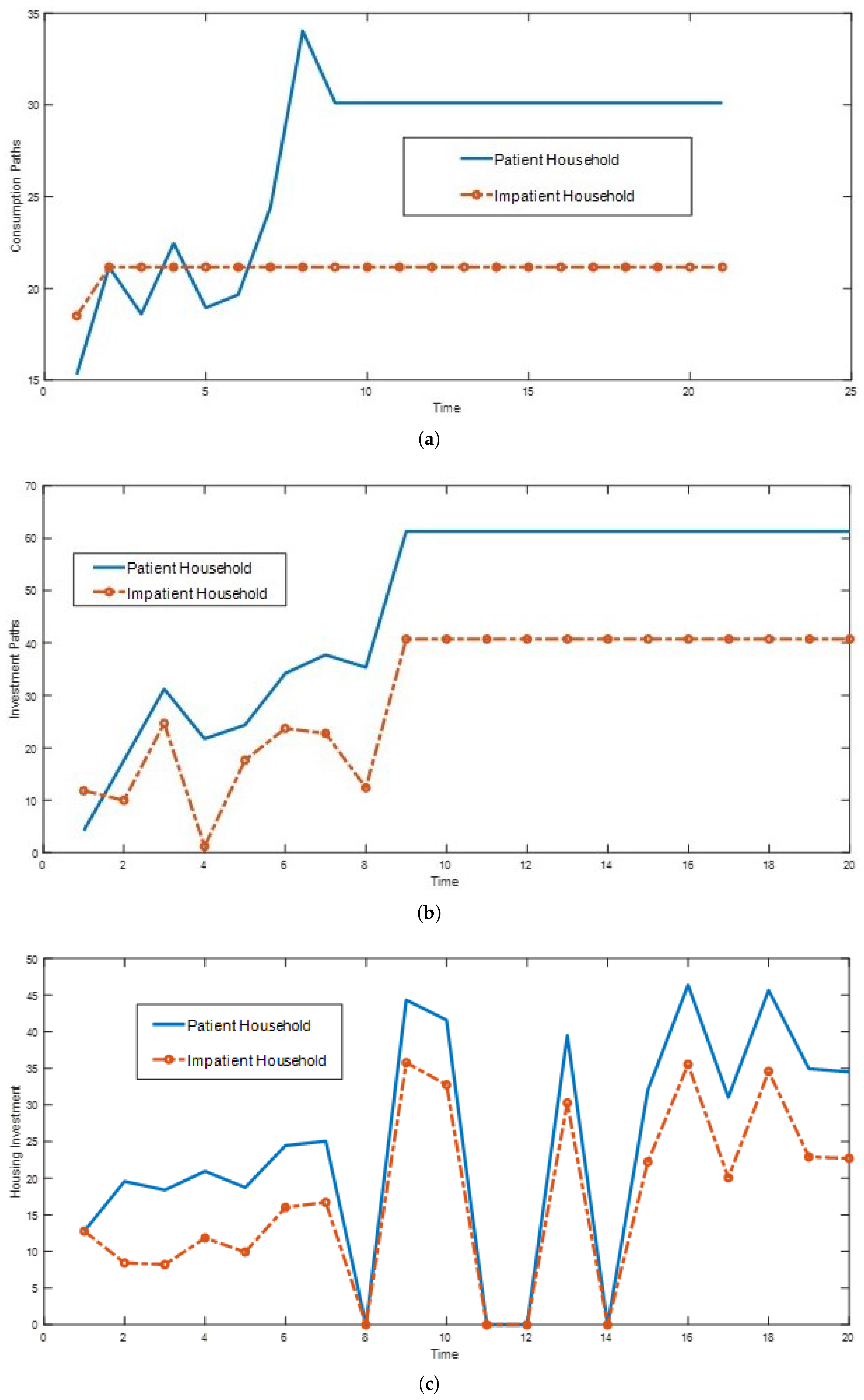
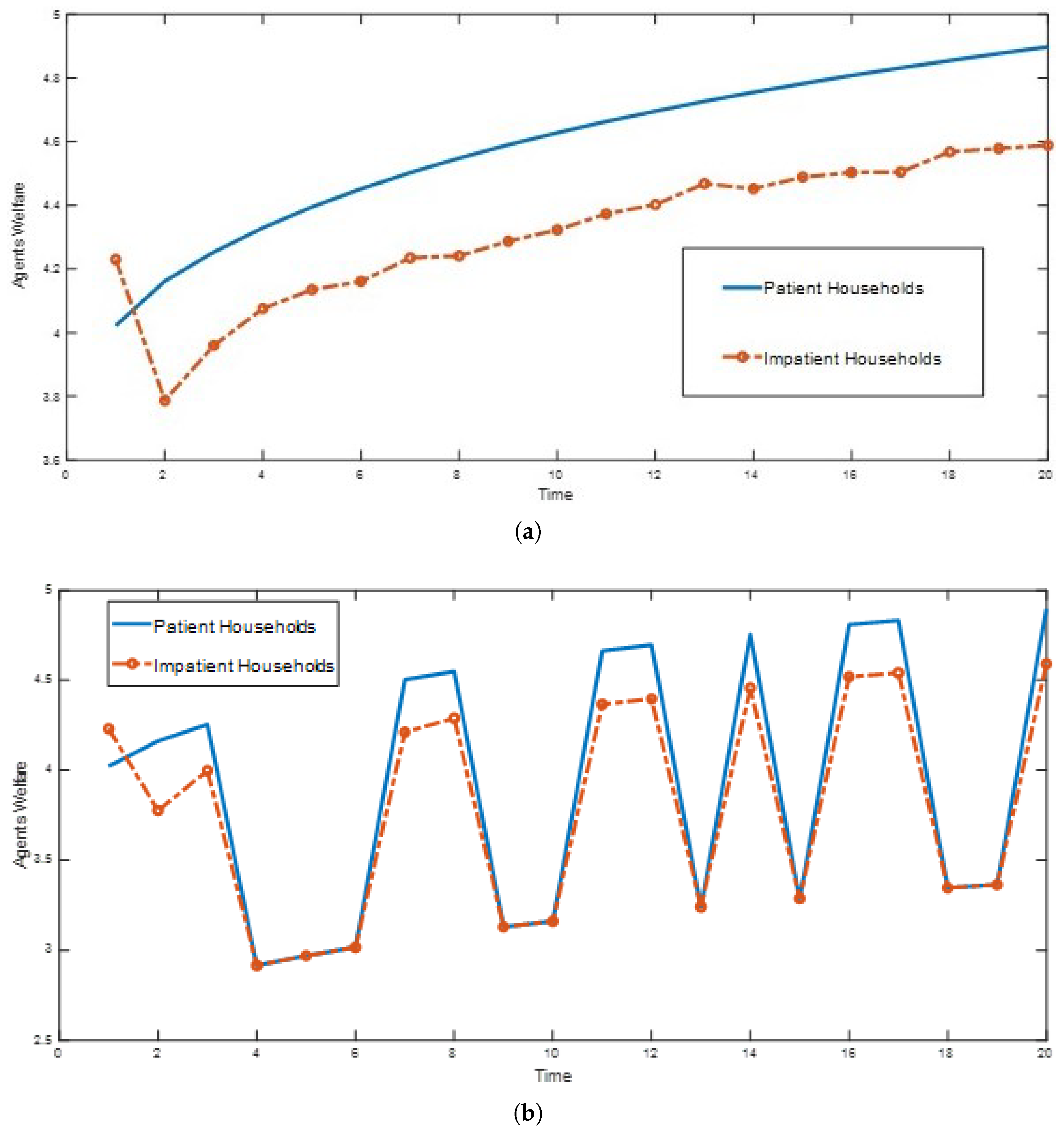
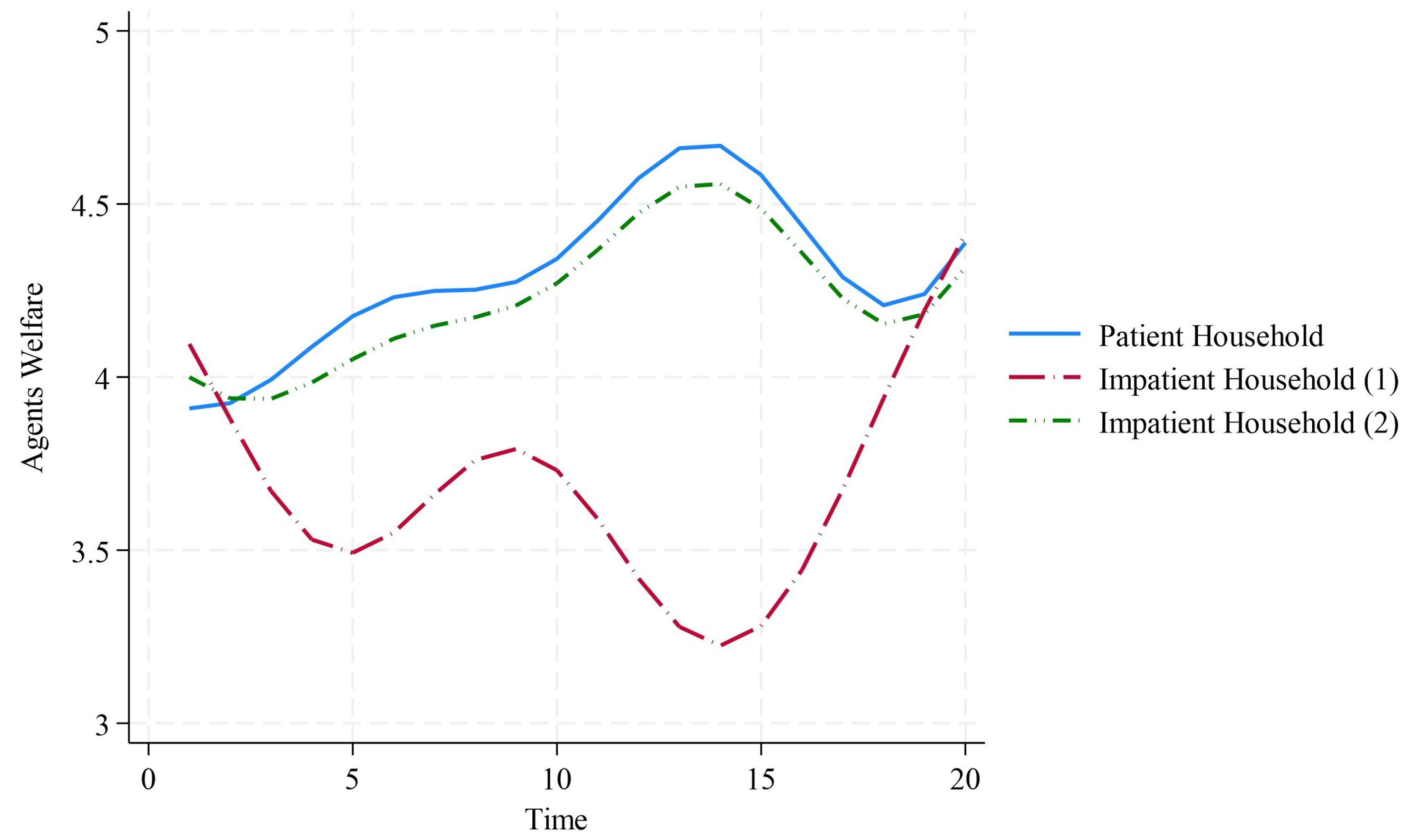
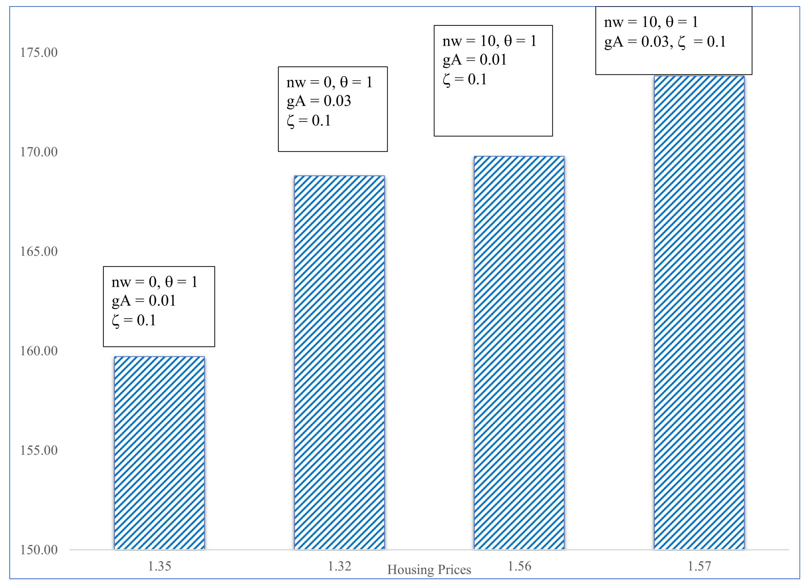
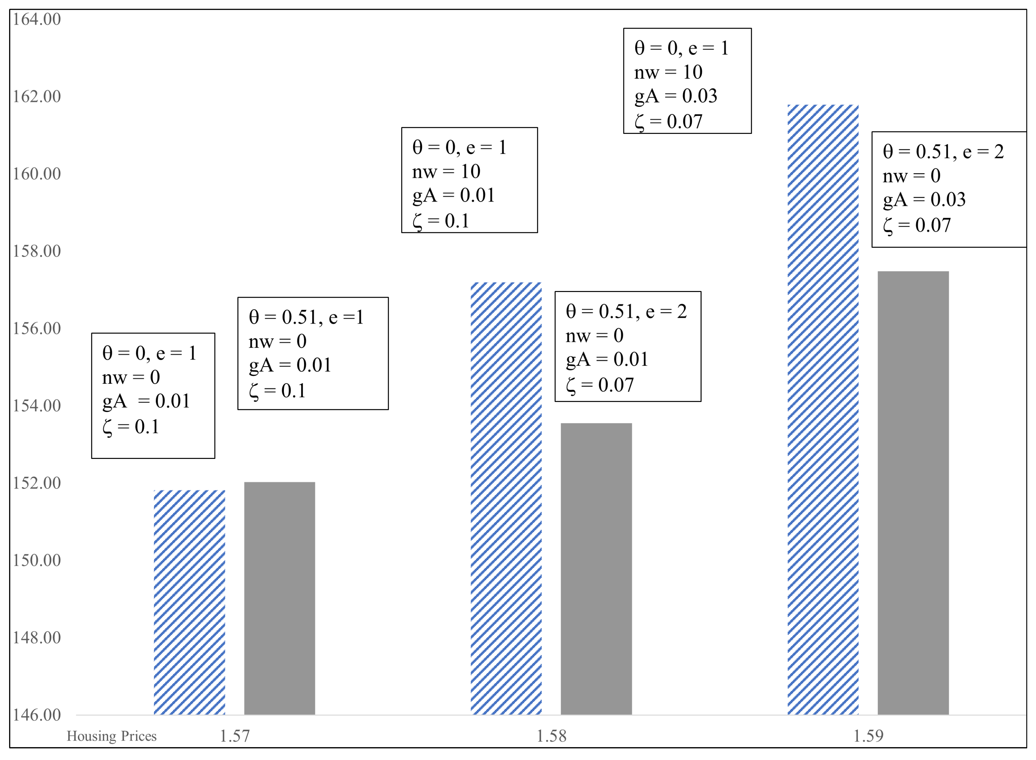
5. Numerical Analysis

To evaluate the primary analytical properties of the model, we utilized the tools of Christiano et al. (2014) and Bora and Zhong (2023). Specifically, we examined agents’ investment and consumption decisions in an economy exposed to domestic and external shocks (credit cycles). To calibrate the theoretical model, we adopted log-linear household preferences as in Iacoviello (2005). In addition, we considered two types of households, patient and impatient, represented by two agents. The patient (saver) agent can invest in bank deposits and housing shares, whereas the impatient (borrower) agent can only invest in housing shares. The patient agent uses their own funds to finance investments, while the impatient agent borrows from banks.

In any period, households received an idiosyncratic shock

ε

that represented the value of their housing shares. In addition, they were exposed to productivity shocks, intermediate production shocks (capital), and the foreign credit cycle. According to Bora and Zhong (2023), we assumed that this cycle entered the economy through a liquidity shock

θ

and the foreign interest rate

R^{*}

, which modified the domestic rate R27.

In terms of the credit cycle and its aggregate effects, we considered four scenarios: a closed economy (

θ = 0

) with low interest rates (Case 1); a partially open economy (

θ < 1

) with low interest rates (Case 2); an open economy (

θ = 1

) with high interest rates (Case 3); and a partially open economy, with high interest rates (Case 4). For comparison, we used a baseline basic case, which assumed no adjustment costs, an open economy, and low interest rates. Housing investment decisions depended on two types of shocks: (i) those affecting interest rates (originating from the rest of the world), and (ii) idiosyncratic shocks (

ε

) that determined the value and return of housing investments.

For each scenario, we examined three policy interventions: bank capitalization (

n w

), exchange rate devaluation (

Δ e > 0

), and changes in reserve ratios (

ζ

). Furthermore, we evaluated households’ welfare by implementing borrowing limits, a mechanism28 to smooth housing prices, and introducing alternative financial investments for impatient households (a risk-free bond). We used Matlab 2023(b), Stata 18, and R Studio 2024 for the computation and data analysis.

Table 1 presents the values of the main parameters derived from our calculations and the existing literature (Gete, 2020; Quadrini, 2020; Acoling et al., 2022). In the first case, a panel dataset of 45 developed and developing countries was used from 2001 to 2022. Table A2 summarizes the key statistics. We used this dataset’s mean values and standard deviations to generate interest rates, housing prices, and default rates. We performed a regression analysis to support the indicators discussed in the Introduction. As seen in Table A3, Table A4 and Table A5, the results were very robust, suggesting strong correlations between the main endogenous variables and the set of explanatory variables. For example, we obtained an error of −0.5 on average between the observed and predicted interest rate gaps for a selection of developing countries (see Table A6).

To evaluate changes in income distribution, we assumed that initially both agents received an equal proportion of income and held the same share of housing investments, thus

τ = 0.5

and

v_{s} = v_{b}

= 0.5

. For simplicity, the model was expressed in per capita terms and units of consumption goods. At the aggregate level, it behaved similarly to a real business cycle model but with two sectors of final production: consumption goods and housing. Agents’ welfare derived from consumption in both sectors.

Idiosyncratic shocks to housing and firms,

ε

and

ϰ

, were generated according to Bora and Zhong (2023), in which mean values and standard deviations coincided with the data (see Table A2).

In particular, the shock

ϰ

influenced the default rate of the rental firms, following a log-normal distribution (see Figure A1). The parameters

μ_{ϰ}

and

σ_{ϰ}

characterized that distribution. The initial domestic liquidity was established with

n w = 0

, and foreign credit was fixed at

b^{*} = 10

. Two productivity growth rates were considered: high (

g A = 0.03

) and low (

g A = 0.01

).

The results are summarized in Table 2, Table 3, Table 4, Table 5 and Table 6, and Figure 4, Figure 5, Figure 6, Figure 7, Figure 8, Figure 9, Figure 10, Figure 11, Figure 12, Figure 13 and Figure 14. For clarity, we summarized the results of the tables in Figure 15, Figure 16 and Figure 17. In Table 2 (basic case), we compare the agents’ allocations under adverse (

ε_{s}

< 1

) and favorable idiosyncratic shocks (

ε_{s}

> 1

), see panels A and B, respectively, where the data indicate that, although housing prices (S) tend to increase under low-interest-rate scenarios, adverse idiosyncratic shocks (

ε_{s} < 1

) cause the patient households to save more in bank deposits than in housing shares, thereby increasing domestic liquidity.

Higher domestic liquidity provides more resources to impatient agents for housing investments, resulting in higher income levels for these agents compared to patient households, especially when productivity growth is faster (panel A). In contrast, favorable shocks reduce domestic liquidity, constraining credit availability for impatient households and firms (panel B). This contraction redistributes wealth, increasing income for savers and decreasing it for borrowers.

Comparing panels A and B in Table 2, we observe that although aggregate wealth may be higher on average when

ε_{s}

> 1

, aggregate output tends to grow faster with increased domestic liquidity.

The results of the basic case suggest that idiosyncratic shocks and adjustment costs induce redistribution and aggregate effects, leading to inefficiencies caused by distress (see Figure 4). Although low-interest-rate scenarios do not guarantee faster growth, Figure 5a,b demonstrate that both efficiency and stability deteriorate as interest rates rise.

Next, we analyzed policy tools assuming favorable housing shocks (

ε_{s} > 1)

that promoted housing investment among patient households but decreased domestic liquidity (see Table 3, Table 4, Table 5 and Table 6).

In Case 1 (Table 3), we examined the impact of changes in bank capitalization (see Stein, 2021), from

n w = 0

(panel A) to

n w = 10

(panel B), reductions in reserve ratio

ζ

(from

0.1

to

0.07

, panels B and C). The results indicated that these measures did not fully compensate for the reduction in liquidity compared to the basic case (panels A and B). The key variable influencing the results appeared to be the shock value

ε

that drove the housing demand of the patient household, with a higher productivity growth yielding better results.

In Case 2 (Table 4), the effects of the exchange rate devaluation (from

e = 1

to

e = 2

) and adjustments to the reserve ratio were analyzed. The results showed that, although the improvements were modest, both the level and the growth rate of aggregate wealth increased, and the income inequality between households decreased. Higher productivity growth amplified these benefits.

Figure 6a,b compare agents’ welfare with full foreign liquidity, under low- and high-interest-rate scenarios. In addition, Figure 7a–c illustrate that optimal investment decisions for housing, savings, and consumption differ between agents. The impatient household tends to consume more in the short term, while the patient household achieves higher long-term consumption and investment paths. Housing shocks induce significant volatility in housing investment for both types of agents.

During adverse shocks to the foreign interest rate (

R^{*}

), Cases 3 and 4 (Table 5 and Table 6) show that domestic interest rates spiked, ranging between 1.23 and 1.33.29

Higher deposit and lending rates depress housing prices: for savers, investing in bank deposits becomes more attractive than housing; for borrowers, increased borrowing costs make housing investment less affordable. Although domestic credit remains abundant, high interest rates limit borrowing for the impatient household and firms, reducing housing investment, output, and aggregate wealth (see panels A in Table 5 and Table 6).

Macroprudential policies become more challenging under high interest rates, especially if rates are exogenous. Measures to increase domestic liquidity or limit foreign capital are less effective, and strategies aimed at reducing borrowing costs, such as those implemented during the COVID-19 pandemic (see Adrian et al., 2023), may be more appropriate when the central bank has limited autonomy or the economy is experiencing an inflationary phase.

Among the measures, we reduced the reserve ratio from 0.07 to 0.03 and implemented a more aggressive devaluation (from

e = 1

to

e = 3

), as shown in panels B of Table 5 and Table 6, respectively. As a result, we observed a reduction in lending rates by nearly 0.8 points compared to the results in panels A, along with increases in both the levels and growth rates of aggregate wealth. Similarly to previous cases, the policy intervention led to a more egalitarian income distribution, increasing the income of the impatient agent relative to the patient agent. Furthermore, higher productivity rates contributed to higher levels and growth rates of wealth (see panel C in Table 3, Table 4 and Table 5).

Comparing the four cases analyzed here, the results indicate that periods of high interest rates are more adverse for the economy than periods of low interest rates, especially when interest rates are exogenous and not aligned with macrofundamentals. Figure 6a,b demonstrate that low interest rates enable agents to achieve higher and more stable levels of welfare than high interest rates, particularly when there is full foreign liquidity.

Although housing prices tend to increase during periods of low interest rates—causing volatility—the scope for macroprudential policy is greater than under high-rate scenarios. For instance, measures such as banks’ capitalization and policies aimed at increasing domestic liquidity can be useful to offset credit constraints caused by adverse foreign shocks and the diversion of financial resources to the real estate sector. In contrast, during periods of high interest rates, policies focused on reducing debt costs become more critical.

Regarding volatility, Figure 7a–c illustrate short-term fluctuations in consumption and investment decisions at the household level, assuming full foreign liquidity (

θ = 1

). This volatility is exacerbated in housing investment, as shown in Figure 7c.

When foreign liquidity is restricted (

θ < 1

), not only does efficiency decrease due to shocks, but aggregate wealth also becomes more volatile as interest rates increase (see Figure 8 and Figure 9a,b.

Optimal decision-making by agents also changes in the presence of imperfect foreign liquidity, as examined in Table 3, Table 4 and Table 5. Figure 10a–c show that the impatient household tends to over-consume in the long term, whereas the patient household invests more in housing. Despite increased volatility at high interest rates, the patient household generally enjoys higher welfare than the impatient household (see Figure 11a,b).

In Figure 12, Figure 13 and Figure 14, we examined the welfare of the agents by applying different measures: a debt limit for the impatient household, a smoothing mechanism for housing prices, and a risk-free bond for the impatient household. We considered full foreign liquidity and high interest rates in the three cases. As illustrated in the figures, limiting borrowing improved welfare for the impatient household during downturns or adverse shocks; however, without intervention, agents were better off in all other periods (see Figure 12). A similar improvement was observed when housing prices were smoothed (see Figure 13). When the impatient agent could save on a risk-free asset as an alternative to housing, as shown in Figure 14, the welfare improved, and both agents, the patient and the impatient, benefited from this intervention. These results can reinforce those previously found. As Figure 15, Figure 16 and Figure 17 summarize, agents’ welfare increased with domestic liquidity in the three scenarios: basic case (Table 2), low interest rates (Table 3 and Table 4), and high interest rates (Table 5 and Table 6).

6. Conclusions

Departing from the existing business cycle literature on financial market frictions, we developed a general equilibrium model to analyze the dynamics of housing and the macroeconomy of an open economy exposed to the global credit cycle. Considering heterogeneous agents (patient and impatient) and two types of savings instruments, bank deposits, and real estate, this framework can be suitable for economies with different degrees of domestic financial development and a variety of integration status with international markets.

Among other contributions, this article developed a dynamic macroeconomic model incorporating an embedded housing production sector with imperfect competition in the banking sector. In the model, investment returns were uncertain, and demand was endogenously determined by households’ preferences, relative prices, interest rates, and income. This structure enabled the model to capture stylized housing and aggregate dynamics observed in advanced and emerging economies.

Second, the analysis identified the conditions under which domestic liquidity-enhancing policies—such as bank capitalization, reserve ratios, and currency devaluation—succeeded or failed in stabilizing investment and output. In particular, the effectiveness of these tools is critically dependent on the level of foreign interest rates and liquidity. In high-interest-rate scenarios, alternative measures, such as stabilizing the price of housing and risk-free bonds, are preferable.

Third, the results demonstrated robust findings across various model calibrations and highlighted the asymmetric effects of foreign liquidity shocks. Foreign liquidity can reinforce or override domestic policy instruments, depending on the level of financial development. These findings imply that capital control measures should be designed by considering the external interest rate environment and the depth of the domestic market, particularly those that target inflow restrictions. Combining micro- and macro-level interventions would be preferable, especially for developing countries with less developed financial markets.

Consequently, facing multiple challenges, these countries must attenuate external shocks and develop local financial markets. They must also control debt and guarantee access to market housing for middle- and low-income groups. Promoting domestic savings in other instruments than real estate would help households and entrepreneurs attenuate price fluctuations. For example, developing a market for bonds, such as green bonds, fintech, and microfinance, would complement other measures such as government subsidies.

Some of these measures were adopted during the COVID-19 pandemic, although significant levels of government and private debt accompanied them. Today, the challenge is to guarantee macroeconomic and financial stability with an affordable market.

These novel insights help explain the housing dynamics and poor growth performance observed in several developing countries during low foreign interest rates. This is particularly relevant in evolving policy shocks in major economies.

The policy design would be limited because we did not include a secondary financial market in our model, and other characteristics that affect the dissemination of shocks (for example, geographical aspects, climate change, and technological shocks). Future research should address these aspects and a wider variety of transmission mechanisms.

Author Contributions

Conceptualization, M.E.F.; Methodology, M.E.F.; Validation, D.R.G. and M.E.F.; Formal analysis, M.E.F.; Investigation, M.E.F. and D.R.G.; Writing—original draft preparation, M.E.F. and D.R.G.; Writing—review and editing, D.R.G. and M.E.F.; Supervision, M.E.F. All authors have read and agreed to the published version of the manuscript.

Funding

This research received no external funding.

Data Availability Statement

Data is contained within the article.

Acknowledgments

We appreciate the comments and suggestions of the conference participants at the World Finance Conference, Malta 2020, and the seminar participants at the Chilean Central Bank, the Universidad de Chile, and the Universidad Alberto Hurtado. The authors thank Eloy Alvarado for computational solutions and Alexis Alfaro for research assistance, Universidad Técnica Federico Santa María.

Conflicts of Interest

The authors declare no conflict of interest.

Appendix A. Proofs

Appendix A.1. The Phillips Curve

From Section 3.2.1, we have the problem:

max E_{0} {\sum_{t = 0}^{\infty} Λ_{i, 0, t} [(\frac{P_{j, t}}{P_{t}} - m c_{t}) y_{j, t} - \frac{λ}{2} {(\frac{P_{j, t}}{P_{j, t - 1}} - 1)}^{2} Y_{t}}

and the first-order conditions (FOCs),

π_{t} (1 + π_{t}) = \frac{1}{λ} (1 - v + v m c_{t}) + β E_{t} (1 + π_{t + 1}) π_{t + 1} Y_{t + 1} / Y_{t}

(A1)

where

\frac{P_{j, t}}{P_{t}} = π_{t}

and

λ

is the adjustment costs’ parameter. In the steady state, we have the following:

(1): $1 + π_{t} = 1$ , then $π_{t} = 0$ , which implies $P_{i t} = P_{t} = P_{s s}$ , for all t and i = 1...n. This implies that prices are constant in the steady state.
(2): With constant prices, we have the following:

π_{t} = π_{t + 1} = π_{s s} = 0

in the steady state, and from FOCs, the marginal cost of production follows

m c_{s s} = \frac{v - 1}{v}

(A2)

Performing

{\hat{m c}}_{t} = (m c_{t} - m c_{s s}) / m c_{s s}

and

ϰ = (v - 1) / λ

, with a little algebra, we obtain

ϰ \hat{m} c_{t} = (1 - v + v m c_{t}) / λ

Linearizing the FOCs around the steady state and doing a little algebra, the Phillips curve becomes (see Aoki et al., 2018)

{\hat{π}}_{t} = ϰ {\hat{m c}}_{t} + β E_{t} {\hat{π}}_{t + 1}

(A3)

Proof.

with

\hat{ϰ} = (x - x_{s s}) / x_{s s}

. □

Appendix A.2. Rental Capital

From Section 3.2.2, the problem of a rental capital firm j follows:

max_{{k_{t}^{f}, b_{t}^{f}, {\bar{ϰ}}_{j, t + 1}}} E_{t} Λ_{i, t, t + 1} {(1 - Γ ({\bar{ϰ}}_{j, t + 1})) R_{t + 1}^{k} q_{t} k_{j, t}}

subject to

q_{t} k_{j, t}^{f} = n_{j, t} + b_{j, t}^{k}

(A4)

and the lender’s participation constraint

E_{t} {G ({\bar{ϰ}}_{j, t + 1}) R_{t + 1}^{k} q_{t} k_{j, t}^{f}} \geq R_{t}^{l} b_{j, t}^{k}

(A5)

Using

G ({\bar{ϰ}}_{j, t + 1}) = Γ ({\bar{ϰ}}_{j, t + 1}) - μ Γ_{u} ({\bar{ϰ}}_{j, t + 1})

and solving through a Lagrangian function, we obtain

L = E_{t} Λ_{i, t, t + 1} {(1 - Γ ({\bar{ϰ}}_{j, t + 1})) R_{t + 1}^{k} q_{t} k_{j, t}} + λ_{1 t} [n_{j, t} + b_{j, t}^{k} - q_{t} k_{j, t}^{f}] - λ_{2 t} [R_{t}^{l} b_{j, t}^{k} - G ({\bar{ϰ}}_{j, t + 1}) R_{t + 1}^{k} q_{t} k_{j, t}^{f}]

Consider the following:

(i): $\partial L / \partial k_{j, t}^{f} = 0$ ;
(ii): $\partial L / \partial b_{j, t}^{k} = 0$ ;
(iii): $\partial L / \partial {\bar{ϰ}}_{j, t + 1} = 0$ .

Then, the FOCs become

R_{t + 1}^{k} = Θ ({\bar{ϰ}}_{j, t + 1}) R_{t}^{l}

(A6)

Proof.

with

Θ ({\bar{ϰ}}_{j, t + 1}) = \frac{Γ^{'} ({\bar{ϰ}}_{j, t + 1})}{[Γ^{'} ({\bar{ϰ}}_{j, t + 1}) G ({\bar{ϰ}}_{j, t + 1}) + G^{'} ({\bar{ϰ}}_{j, t + 1}) (1 - Γ ({\bar{ϰ}}_{j, t + 1}))]} > 0

, which represents the risk related to rental-capital investment. □

Appendix A.3. Interest Rates

From the definitions of Section 3.2 and Section 3.3, we see that the nominal lending interest rate follows

(1 + i_{t}^{l}) = R_{t + 1}^{l} π_{t + 1}

(A7)

with

{\hat{π}}_{t + 1} = ϰ {\hat{m c}}_{t + 1} + β E_{t} {\hat{π}}_{t + 2}

. Taking the logs of both sides of Equation (46), we obtain log

(1 + i_{t}^{l}) = log R_{t + 1}^{l} + log π_{t + 1}

.

Under perfect competition, we have

R_{t}^{l} = R_{t}^{l} / θ

; thus,

(1 + i_{t}^{l}) / π_{t + 1} = (1 / θ) (1 + i_{t}^{*}) / π_{t + 1}^{*}

, where

i_{t}^{*}

is the nominal foreign interest rate, and

π_{t + 1}^{*}

is foreign inflation. Taking the logs of both sides of this expression, we obtain the following:

{\tilde{i}}_{t} = {\tilde{i^{*}}}_{t} + {\tilde{γ}}_{E_{t + 1}} + Y_{t}

(A8)

where

{\tilde{i}}_{t} = log (1 + i_{t}^{l})

,

{\tilde{i^{*}}}_{t} = log (1 + i_{t}^{*})

, and

γ_{E_{t + 1}} = γ_{e_{t + 1}} + (π_{t + 1}^{*} - π_{t + 1})

, which denotes the expected devaluation at time

t + 1

, with

γ_{e_{t + 1}}

being the real devaluation at this time.

Y_{t}

= l o g (1 / θ_{t})

.

In the case of Cournot competition, when there is perfect foresight, local interest rates behave as

{\tilde{i}}_{t} = {\tilde{i^{*}}}_{t} + {\tilde{γ}}_{E_{t + 1}} + Y_{t} + \tilde{Ξ}

Proof.

where

\tilde{Ξ} = 1 / [1 - \frac{1}{N η_{l}^{D}}]

denotes the degree of market power in the banking sector. □

Table A1. Housing deficits in selected countries.

Developed Countries
	Deficit	Population	Financing
	(Millions)		(%)
Finland	0.6	5.6	70
Germany	0.7	83.3	90
Greece	0.2	10.4	70–75
Portugal	0.1	10.9	60–70
United Kingdom	4.3	68.4	80–95
Developing Countries
	Deficit	Population	Financing
	(Millions)		(%)
Argentina	4.0	46.2	50–70
Brazil	5.8	215.3	80
Chile	0.6	19.6	75
Colombia	5.2	51.9	70
Mexico	2.2	127.5	80–90
India	47.0	1417	85

Note: Housing deficit can include units in poor conditions or of poor quality. Source: Bank of Mexico (2024); Central Bank of Argentina (2024); Casen (2022); Central Bank of Brazil (2024); Central Bank of Chile (2024); Central Bank of Colombia (2024); DANE (2024); Instituto Brasileiro de Geografia e Estatistica (2024); Mordor Intelligence (2024); OECD (2023); World Bank (2021).

Table A2. Main basic statistics.

Variable	Observations	Mean	Std. Dev.	Min	Max
Central Bank Interest Rate	946	5.7	12.3	0.0	316.0
Credit to GDP (Percentage)	926	107.0	69.5	8.0	288.5
Current Account to GDP (Percentage)	985	−0.5	5.8	−30.9	28.0
Deposit Interest Rate (Percentage)	862	4.7	6.4	0.0	74.7
Devaluation Rate (Percentage)	944	1.3	15.0	−272.2	120.0
Fed Fund Interest Rate (Percentage)	990	1.4	1.5	0.1	5.0
Foreign Reserves (USD Millions)	986	108,160	392,610	195	3,900,000
Gap Between Interest Rates	946	4.3	12.3	−2.2	314.3
Household Debt to GDP (Percentage)	771	50.1	31.0	2.5	137.4
Index of Housing Cost (Base Year = 2015)	667	100.7	24.3	12.5	178.5
Inflation Rate (Percentage)	914	4.1	5.3	−3.4	93.6
Lending Interest Rate (Percentage)	830	8.9	10.5	0.0	118.4
Money Market Interest Rate (Percentage)	745	4.4	6.2	−0.6	86.1
Nominal Exchange Rate (Domestic Currency to USD)	989	536.2	1929.4	0.5	15,731
Nonperforming Loans (Percentage of Debt)	543	4.1	5.3	0.2	45.6
Openness Index 2001–2022	940	69.7	28.7	0.0	100.0
Developed Countries	396	87	10	29	100
Developing Countries	544	57	32	0	100
Per Capita GDP (Constant USD of 2015)	987	24,031	29,724	263	288,275
Private debt to GDP (Percentage)	771	80.0	40.4	12.5	185.3
Real GDP growth	989	2.8	3.6	−21.4	14.0
Total Factor Productivity (Rate of Growth)	665	1.0	0.1	0.8	1.2
Unemployment Rate	871	8.0	5.0	0.0	33.0
U.S. Central bank Rate	990	1.5	1.6	0.1	5.3
VIX	990	20.2	6.2	11.1	31.8
Year	990	2012	6	2001	2022

Note: Index of housing cost is an index number calculated by the OECD that measures the prices of residential properties over time. The gap between interest rates is obtained as the difference between each country’s central bank interest rate and the U.S. policy rate (Federal Fund Rates). Openness index (overall openness index) provides information on the state of openness of the capital account based on 12 types of asset categories, where one implies a fully liberalized economy, and zero implies a closed economy. Source of data: BIS (2023); IMF (2023); OECD (2023).

Table A3. Financial integration.

y_it = a_i + bX_it + v_it
(A): All Countries
	2001–2022		2001–2014		2015–2022
Dependent Variable: D log Credit/GDP_i
D log Credit/GDP_us	0.5196 ***	0.4549 ***	0.3810 **	0.3474 **	1.0388 ***	1.1067 ***
	(0.1066)	(0.0880)	(0.1427)	(0.1244)	(0.1394)	(0.0927)
D log GDPpc	−0.2445 ***	−0.2677 ***	−0.2963 ***	−0.3221 ***	−0.2145 ***	−0.2044 ***
	(0.0248)	(0.0257)	(0.0355)	(0.0367)	(0.0309)	(0.0356)
Adj R²	11%		11%		28%
Chi²		142		80		314
Observations	881	881	543	543	338	338
(B): Developed Countries
	2001–2022		2001–2014		2015–2022
Dependent Variable: D log Credit/GDP_i
D log Credit/GDP_us	0.7553 ***	0.6814 ***	0.5978 ***	0.5412 ***	1.2064 ***	1.1491 ***
	(0.0757)	(0.0577)	(0.0826)	(0.0679)	(0.1371)	(0.0909)
D log GDPpc	−0.0793 ***	−0.0732 **	−0.0922 ***	−0.0839 **	−0.1164 ***	−0.2652 ***
	(0.0223)	(0.0236)	(0.0274)	(0.0284)	(0.0344)	(0.0495)
Adj R²	21%		18%		39%
Chi²		141		64		260
Observations	377	377	233	233	144	144
(C): Developing Countries
	2001–2022		2001–2014		2015–2022
Dependent Variable: D log Credit/GDP_i
D log Credit/GDP_us	0.2298	0.1773	0.0573	0.0381	0.8373 ***	1.0595 ***
	(0.1745)	(0.1468)	(0.2351)	(0.2064)	(0.2214)	(0.1502)
D log GDPpc	−0.3202 ***	−0.3479 ***	−0.3757 ***	−0.4088 ***	−0.2798 ***	−0.1947 ***
	(0.0361)	(0.0372)	(0.0515)	(0.0533)	(0.0455)	(0.0491)
Adj R²	13%		14%		27%
Chi²		95		59		145
Observations	504	504	310	310	194	194

Note: Table A3 shows the correlation between variations in the ratio of credit to GDP for each country and corresponding changes in the U.S. ratio. We estimated the regression utilizing changes in per capita GDP as a control variable. In panel A, the table shows the correlations for the full sample of data, and panel B shows the correlations for the group of developing countries. The coefficients indicate the direction and the importance of the correlation. For example, 0.5196 in column 1 of panel A (2001–2022) indicates that each country’s credit-to-GDP ratio increases 0.52 percent (approximately) when the U.S. ratio increases 1 percent. In column 5, the country´s ratio on the right increases by 1.03 percent. In columns 2, 4, and 6, Chi2 is the value of the Wald test. **: significance at 5%; ***: significance at 1%.

Table A4. Household debt and housing prices.

y_it = a_i + bX_it + v_it
(A): All Countries
	2001–2022		2001–2014		2015–2022
Dependent Variable: Household Debt to GDP (log)
Housing Price (log)	0.6043 ***	0.6515 ***	0.6752 ***	0.6704 ***	0.0800	0.3458
	(0.0665)	(0.0724)	(0.0842)	(0.0757)	(0.2804)	(0.2606)
Exchange Rate (log)	−0.0658 ***	−0.0679 ***	−0.0567 ***	−0.0639 ***	−0.0780 ***	−0.0709 ***
	(0.0091)	(0.0093)	(0.0117)	(0.0119)	(0.0146)	(0.0149)
Openness	0.9040 ***	0.8631 ***	1.0008 ***	0.9319 ***	0.7714 ***	0.7813 ***
	(0.0849)	(0.0829)	(0.1109)	(0.1068)	(0.1343)	(0.1316)
Unemployment Rate	−0.0210 ***	−0.0070 *	−0.02497792 **	−0.0062	−0.0192 **	−0.0097 *
	(0.0044)	(0.0030)	(0.0059)	(0.0042)	(0.0071)	(0.0046)
Adj R²	38%		43%		28%
Chi²		468		352		103
Observations	612	612	387	387	225	225
(B): Developed Countries
	2001–2022		2001–2014		2015–2022
Dependent Variable: Household Debt to GDP (log)
Housing Price (log)	0.2565 **	0.2323 **	0.2453 *	0.1408	0.2867	0.3612
	(0.0880)	(0.0875)	(0.1096)	(0.1065)	(0.2647)	(0.2365)
Exchange Rate (log)	0.0217	0.0483 **	−0.0059	0.0478 **	0.0478 **	0.0666 ***
	(0.0117)	(0.0154)	(0.0176)	(0.0213)	(0.0174)	(0.0196)
Openness	−0.2246	−0.3175	−0.4175	−0.6568 **	0.1617	0.1474
	(0.1932)	(0.1840)	(0.2566)	(0.2349)	(0.3403)	(0.2704)
Unemployment Rate	−0.0146 **	−0.0201 ***	−0.0275 **	0.0028	−0.0153 *	−0.0088 **
	(0.0047)	(0.0032)	(0.0088)	(0.0044)	(0.0066)	(0.0044)
Adj R²	6%		6%		12%
Chi²		27		12		31
Observations	382	382	216	216	130	130
(C): Developing Countries
	2001–2022		2001–2014		2015–2022
Dependent Variable: Household Debt to GDP (log)
Housing Price (log)	0.6779 ***	0.7394 ***	0.6784 ***	0.7447 ***	1.1125 **	1.0107 **
	(0.0866)	(0.0726)	(0.1025)	(0.0855)	(0.3508)	(0.2902)
Exchange Rate (log)	−0.0458 ***	−0.0273 **	−0.0390 *	−0.0212	−0.04316 *	−0.0157
	(0.0117)	(0.0094)	(0.0152)	(0.0135)	(0.0178)	(0.0189)
Openness	0.1514	0.3334 ***	0.4515 **	0.5995 ***	−0.3936 *	−0.3095
	(0.1055)	(0.0972)	(0.1375)	(0.1209)	(0.1666)	(0.1734)
Unemployment Rate	0.0077	0.0132 **	0.0056	0.0185 **	0.0160	0.0152 **
	(0.0061)	(0.0043)	(0.0087)	(0.0065)	(0.0090)	(0.0058)
Adj R²	25%		30%		14%
Chi²		127		16		12
Observations	230	230	135	135	95	95

Note: Table A4 shows the correlation between household debt, housing prices (housing cost index), and exchange rates. We estimated the regression by OLS, utilizing openness and the unemployment rate as control variables. In panel A, the table shows the correlations for the full sample of data, panel B shows the correlations for the group of developed countries, and panel C the group of developing countries. The coefficients indicate the direction and the importance of the correlation. For example, 0.6043 in column 1 of panel A (2001–2022) indicates that household debt increases 0.6 percent (approximately) when the housing prices increase 1 percent. In panel C, debt increases by 0.68 percent. In columns 2, 4, and 6, Chi2 is the value of the Wald test. *: significance at 10%; **: significance at 5%; ***: significance at 1%.

Table A5. Gap between interest rates and macroeconomic variables.

y_it = a_i + bX_it + v_it
(A): All Countries
	2001–2022		2001–2014		2015–2022
Dependent Variable: Gap Between Interest Rates
$Δ$ log Ex Rate_t	3.1775 ***	2.1920 **	2.3839 *	1.9756 *	5.2248 *	1.1037
	(0.8954)	(0.6925)	(0.9691)	(0.8294)	(2.2642)	(1.8741)
$Δ$ log Ex Rate_t+1	1.5258	0.5224	1.6263	0.5991	−0.2961	−5.4699
	(0.8942)	(0.6976)	(0.9619)	(0.8416)	(2.2264)	(1.8079)
Inflation_t	0.7489 ***	0.7545 ***	0.7301 ***	0.7557 ***	0.7133 ***	0.6490 ***
	(0.0592)	(0.0584)	(0.0684)	(0.0720)	(0.1190)	(0.1044)
Inflation_t−1	0.4448 ***	0.3807 ***	0.3921 ***	0.3551 ***	0.6151 ***	0.7657 ***
	(0.0543)	(0.0520)	(0.0610)	(0.0631)	(0.1134)	(0.1119)
Dummy low growth	0.8024 **	0.5041	0.1834	0.7383 ***	1.7388 ***	0.9995 ***
	(0.3089)	(0.2775)	(0.3865)	(0.4267)	(0.5083)	(0.3339)
Adj R²	54%		52%		59%
Chi²		915		506		623
Observations	802	802	499	499	303	303
(B): Developed Countries
	2001–2022		2001–2014		2015–2022
Dependent Variable: Gap Between Interest Rates
$Δ$ log Ex Rate_t	0.1917	1.3289	−0.2366	0.7776	3.0196 **	2.9055 **
	(0.7861)	(0.8719)	(1.0027)	(1.1313)	(1.0756)	(1.0128)
$Δ$ log Ex Rate_t+1	2.5259 **	2.3153 **	2.2381 *	2.9505 **	3.6886 **	2.6114 *
	(0.8307)	(0.9142)	(1.0741)	(1.1300)	(1.2329)	(1.1552)
Inflation_t	0.2314 ***	0.2194 **	0.1890 *	0.1967	0.0508	0.1726 *
	(0.0653)	(0.0766)	(0.0917)	(0.1106)	(0.0893)	(0.0754)
Inflation_t−1	0.2373 ***	0.1947 **	0.1452	0.1278	−0.1007	−0.1854 **
	(0.0671)	(0.0736)	(0.0940)	(0.1015)	(0.0929)	(0.0790)
Dummy low growth	0.2088	0.0167	0.1013	0.2621	0.0748	0.0423
	(0.1593)	(0.1594)	(0.2068)	(0.2340)	(0.2115)	(0.1730)
Adj R²	12%		3%		9%
Chi²		34		13		26
Observations	342	342	216	216	126	126
(C): Developing Countries
	2001–2022		2001–2014		2015–2022
Dependent Variable: Gap Between Interest Rates
$Δ$ log Ex Rate_t	3.4332 **	2.2067 *	2.8720 *	2.2097 *	4.8284	6.7914 *
	(1.2127)	(0.8998)	(1.2986)	(1.0568)	(3.2854)	(2.7618)
$Δ$ log Ex Rate_t+1	0.8570	−0.0293	1.0811	1.0126	−1.2860	−4.5774
	(1.1942)	(0.9065)	(1.2766)	(1.0716)	(3.0984)	(3.1582)
Inflation_t	0.7250 ***	0.7269 ***	0.7092 ***	0.6904 ***	0.6772 ***	0.5884 ***
	(0.0785)	(0.0760)	(0.0914)	(0.0946)	(0.1588)	(0.1320)
Inflation_t−1	0.3588 ***	0.3265 ***	0.2912 ***	0.2987 ***	0.5662 ***	0.6210 ***
	(0.0714)	(0.0676)	(0.0804)	(0.0806)	(0.1526)	(0.1270)
Dummy low growth	2.3424 ***	1.3633 **	2.2400 **	3.4648 ***	2.3985 **	1.7599 *
	(0.5778)	(0.5122)	(0.8632)	(0.9899)	(0.8135)	(0.6484)
Adj R²	46%		43%		51%
Chi²		387		219		241
Observations	460	460	283	283	177	177

Note: Table A5 shows the correlation between the gap between interest rates (measured as the differences in central bank’s interest rates and the U.S. central bank rate), current exchange rate devaluations (

Δ

log Ex Rate_t), expected devaluation (

Δ

log Ex Rate_t+1), current inflation, and lagged inflation. We estimated the model by OLS, utilizing a dummy variable of low growth as a control variable. The table shows the correlations for the full sample of data in panel A, for the group of developed countries in panel B, and for the group of developing countries in panel C. The coefficients indicate the direction and the importance of the correlation. For example, 3.1775 in column 1 of panel A (2001–2022) indicates that the gap between interest rates increases 3.18 times when there is a currency devaluation. In panel C, this rise would be 3.43. In columns 2, 4, and 6, Chi2 is the value of the Wald test. *: significance at 10%; **: significance at 5%; ***: significance at 1%.

Table A6. Gaps between interest rates.

Selected Countries	Observed	Predicted	Difference
Bolivia	2.42	2.97	−0.55
Brazil	7.24	7.28	−0.04
Chile	2.48	4.10	−1.62
China	1.94	1.79	0.16
Colombia	3.91	4.88	−0.96
Costa Rica	2.13	1.59	0.54
Hungary	1.12	2.22	−1.09
India	4.88	5.05	−0.17
Average	3.27	3.73	−0.47

Note: Table A6 displays the observed and predicted annual gaps between interest rates for a selected group of countries, based on the results of Table A5.

Figure A1. Gamma distribution of non-performing loans (default rate).

Figure A2. Data-structure model diagram.

Notes

1	Measured through the Housing Price Index of the OECD.
2	See Table A1.
3	See for example, the emerging market crises during the 1990s, Mendoza (2002).
4	See Table A2.
5	Accordingly, housing wealth accounted for approximately 50 percent of Chinese households’ net worth between 2004 and 2019.
6	Leading to reversals of capital flows when lending conditions change (Mendoza, 2002; Calvo et al., 2006).
7	For example, the U.S. economy.
8	Directly or indirectly, independently of the exchange-rate regime.
9	Which includes expectations about the future, mortgage rates, house prices, and rental rates.
10	Provided by housing shares, m.
11	And the return.
12	Note that in the absence of the idiosyncratic shock $ε$ , housing would become a safer investment.
13	Including collateral for debt, and full or partial financing.
14	For example, in the case of China (Dong et al., 2021).
15	Coming from housing shares and bank deposits.
16	These shares are recurrent housing expenditures.
17	Given by external conditions, such as natural catastrophes, market conditions, etc., with $0 < ε < ε_{max} .$
18	See Appendix A online.
19	Accumulated assets.
20	We are assuming here that physical capital is homogeneous and is traded under perfect market competition.
21	Expressed by the demand elasticity and the banks’ shares in the market.
22	Which depends on the firms’ own capital n, among other aspects.
23	The degree of market competition would determine the magnitude of this effect.
24	Given the fixed amount of land.
25	Interbank real interest rate.
26	See Appendix A.3.
27	The idea is to represent extreme cases described in the literature, where the global cycle can lead to excessive credit growth in boom times and excessive contraction in bad times (Rey, 2018).
28	Based on taxation in good times and a subsidy in adverse times.
29	Note that the maximum rates reached during the Global Financial Crisis in developing countries were 1.17 and 1.36, respectively.

References

Acoling, A., Hoek-Smit, M., & Green, R. (2022). Measuring the housing sector’s contribution to GDP in emerging market countries. International Journal of Housing Markets and Analysis, 15(5), 977–994. [Google Scholar] [CrossRef]
Adrian, T., Natalucci, F., & Qureshi, M. (2023). Macro-financial stability in the COVID-2019 crisis: Some reflections. Annual Review of Financial Economics, 15, 29–54. [Google Scholar] [CrossRef]
Aoki, K., Benigno, G., & Kiyotaki, N. (2018). Monetary and financial policies in emerging markets. Working paper. Princeton University. [Google Scholar]
Bank for International Settlements (BIS). (2023). Statistics database. Bank for International Settlements. [Google Scholar]
Bank of Mexico. (2024). Economic information system. Bank of Mexico. [Google Scholar]
Baqaee, D., Farhi, E., & Sangani, K. (2024). The supply-side effects of monetary policy. Journal of Political Economy, 132(4), 1065–1112. [Google Scholar] [CrossRef]
Beraja, M., Fuster, A., Hurst, E., & Vavra, J. (2019). Regional heterogeneity and the refinancing channel of monetary policy. The Quarterly Journal of Economics, 134(1), 109–183. [Google Scholar] [CrossRef]
Bernanke, B., Gertler, M., & Gilchrist, S. (1999). The financial accelerator in a quantitative business cycle framework. In J. B. Taylor, & M. Woodford (Eds.), Handbook of macroeconomics (Vol. I). Elsevier. [Google Scholar] [CrossRef]
Bora, D., & Zhong, M. (2023). Understanding bank and nonbank credit cycles: A structural exploration. Journal of Money Credit and Banking, 55(1), 103–142. [Google Scholar] [CrossRef]
Bruno, V., & Shin, H. S. (2015). Capital flows and the risk-taking channel of monetary policy. Journal of Monetary Economics, 71, 119–132. [Google Scholar] [CrossRef]
Caballero, R., & Krishnamurthy, A. (2008). Collective risk management in a flight to quality episode. The Journal of Finance, 63(5), 2195–2230. [Google Scholar] [CrossRef]
Caballero, R., & Simsek, A. (2022). Monetary policy with opinionated markets. American Economic Review, 112(7), 2353–2392. [Google Scholar] [CrossRef]
Calvo, G. (1983). Staggered prices in a utility-maximizing framework. Journal of Monetary Economics, 12, 383–398. [Google Scholar] [CrossRef]
Calvo, G., Izquierdo, A., & Talvi, E. (2006). Sudden stops and phoenix miracles in emerging markets. American Economic Review, 96(2), 405–410. [Google Scholar] [CrossRef]
Carillo, J., Mendoza, E., Nugher, V., & Roldan Peña, J. (2021). Tight money-tight credit: Coordination failure in the conduct of monetary and financial policies. American Economic Journal: Macroeconomics, 13(3), 37–73. [Google Scholar] [CrossRef]
Casen. (2022). Encuesta caracterización socioeconómica nacional 2020. Ministerio de Desarrollo Social y Familia, Chile. [Google Scholar]
Central Bank of Argentina. (2024). Statistics database. Central Bank of Argentina. [Google Scholar]
Central Bank of Brazil. (2024). Statistics database. Central Bank of Brazil. [Google Scholar]
Central Bank of Chile. (2024). Statistics database. Central Bank of Chile. [Google Scholar]
Central Bank of Colombia. (2024). Statistics database. Central Bank of Colombia. [Google Scholar]
Christiano, L., Ilut, C. L., Motto, R., & Rostagno, M. (2010). Monetary policy and stock market booms. NBER Working Paper 16402. National Bureau of Economic Research. [Google Scholar]
Christiano, L., Motto, R., & Rostagno, M. (2014). Risk shocks. American Economic Review, 104(1), 27–65. [Google Scholar] [CrossRef]
Clarida, R. (2019). The global factor in neutral policy rates: Some implications for exchange rates, monetary policy, and policy coordination. International discussion papers 1244. Board of Governors of the Federal Reserve System. [Google Scholar] [CrossRef]
Cox, J., & Ludvigson, S. C. (2019). Drivers of the great housing boom-bust: Credit conditions, beliefs, or both? NBER working paper No. 25285. National Bureau of Economic Research. Available online: https://www.nber.org/papers/w25285 (accessed on 5 March 2022).
DANE. (2024). National administrative department of statistics, colombia. Housing deficits. DANE. [Google Scholar]
Dong, F., Liu, J., Xu, Z., & Zhao, B. (2021). Flight to housing in China. Journal of Economic Dynamic and Control, 130, 104189. [Google Scholar] [CrossRef]
Duca, J., Muellbauer, J., & Murphy, A. (2021). What drives house price cycles? International experience and policy issues. Journal of Economic Literature, 59(3), 773–864. [Google Scholar] [CrossRef]
Eichenbaum, M., Rebelo, S., & Wong, A. (2022). State-Dependent Effects of Monetary Policy: The Refinancing Channel. American Economic Review, 112(3), 721–61. [Google Scholar] [CrossRef]
Gali, J., & Monacelli, T. (2005). Monetary policy and exchange rate volatility in a small open economy. Review of Economic Studies, 72, 707–734. [Google Scholar] [CrossRef]
Geanakoplos, J. (2016). The credit surface and monetary policy. In Progress and confusion: The state of macroeconomic policy (pp. 143–153). International Monetary Fund and Massachusetts Institute of Technology. MIT Press. [Google Scholar] [CrossRef]
Geanakoplos, J., & Wang, H. (2020). Quantitative easing, collateral constraints, and financial spillovers. American Economics Journal: Macroeconomics, 12(4), 180–217. [Google Scholar] [CrossRef]
Gertler, M., Kiyotaki, N., & Pristino, A. (2016). Wholesale banking and bank runs in macroeconomic modelling of financial crises. In J. Taylor, & H. Uhlig (Eds.), Handbook of macroeconomics (1st ed., Vol. 2, pp. 1345–1425). Chapter 16. Elsevier. [Google Scholar]
Gertler, M., Kiyotaki, N., & Queralto, A. (2012). Financial crises, bank risk exposure and government financial policy. Journal of Monetary Economics, 59(Supplement), 517–534. [Google Scholar] [CrossRef]
Gete, P. (2020). Expectations and the housing boom and bust. An open economy view. Journal of Housing Economics, 49, 101690. [Google Scholar] [CrossRef]
Iacoviello, M. (2005). House prices, borrowing constraints, and monetary policy in the business cycle. American Economic Review, 95(3), 739–764. [Google Scholar] [CrossRef]
Iacoviello, M., & Neri, S. (2010). Housing market spillovers: Evidence from an estimated DSGE model. American Economic Journal: Macroeconomics, 2, 125–164. [Google Scholar] [CrossRef]
Ilzetzki, E., & Jin, K. (2021). The puzzling change in the international transmission of U.S. macroeconomic policy shocks. Journal on International Economics, 130(C), 103444. [Google Scholar] [CrossRef]
IMF. (2023). International monetary fund. international finance statistics. IMF. [Google Scholar]
Instituto Brasileiro de Geografia e Estatistica. (2024). Population and housing statistics. Instituto Brasileiro de Geografia e Estatistica. [Google Scholar]
Kamara, A., & Koirala, N. (2023). The Dynamic Impacts of Monetary Policy Uncertainty Shocks. Economies, 11(1), 17. [Google Scholar] [CrossRef]
Kiyotaki, N., & Moore, J. (1997). Credit cycles. Journal of Political Economy, 105(2), 211–248. [Google Scholar] [CrossRef]
Mendoza, E. (2002). Credit, Prices and Crashes: Business Cycles with a Sudden Stop. In S. Edwards, & J. Frankel (Eds.), Preventing currency crises in emerging markets. Chapter 7. University of Chicago Press. [Google Scholar]
Mian, A., Sufi, A., & Verner, E. (2017). Household Debt and Business Cycles Worldwide. Quarterly Journal of Economics, 132(4), 1755–1817. [Google Scholar] [CrossRef]
Minsky, H. (1986). Stabilizing an unstable economy. Yale University Press. [Google Scholar]
Mordor Intelligence. (2024). Real estate market in india size & share analysis–growth trends & forecasts (2024–2029). Available online: https://www.mordorintelligence.com/industry-reports/real-estate-industry-in-india (accessed on 12 May 2025).
Muellbauer, J. (2024). Housing and macroprudential policy. Economics Series Working Papers 1056. University of Oxford. [Google Scholar]
Ng, E. C. Y., & Feng, N. (2016). Housing market dynamics in a small open economy: Do external and new shocks matter? Journal of International Money and Finance, 63, 64–88. [Google Scholar] [CrossRef]
Obstfeld, M., & Rogoff, K. (1995). Exchange rate dynamics redux. Journal of Political Economy, 103(3), 624–660. [Google Scholar] [CrossRef]
OECD. (2023). Statistics dataset. OECD. [Google Scholar]
Pateiro-Rodriguez, C., Martín-Bermúdez, F., Barros-Campello, E., & Pateiro-Lopez, C. (2025). On the weak impact of base money on broad money in the context of unconventional monetary policy: Euro area 2008–2024. Economies, 13, 130. [Google Scholar] [CrossRef]
Piazzesi, M., & Schneider, M. (2016). Housing and Macroeconomics. In J. Taylor, & H. Uhlig (Eds.), Handbook of Macroeconomics (1st ed., Vol. 2, pp. 1547–1640). Chapter 19. Elsevier. [Google Scholar]
Quadrini, V. (2020). The impact of industrialized countries’ monetary policy on emerging economies. IMF Economic Review, 68, 550–583. [Google Scholar] [CrossRef]
Ramey, V. (2016). Macroeconomic Shocks and their Propagation. In J. Taylor, & H. Uhlig (Eds.), Handbook of Macroeconomics (1st ed., Vol. 2, pp. 71–162). Chapter 2. Elsevier. [Google Scholar]
Reinhart, C., Reinhart, V., & Tashiro, T. (2015). Does reserve accumulation crowd out investment? Journal of International Money and Finance, 63, 89–111. [Google Scholar] [CrossRef]
Rey, H. (2016). International channels of transmission of monetary policy and the Mundellian trilemma. IMF Economic Review, 64(1), 6–35. [Google Scholar] [CrossRef]
Rey, H. (2018). Dilemma not trilemma: The global financial cycle and monetary policy independency. NBER working paper 21162. National Bureau of Economic Research. [Google Scholar]
Rotemberg, J. (1982). Monopolistic price adjustment and aggregate output. The Review of Economic Studies, 49(4), 517–531. [Google Scholar] [CrossRef]
Stein, J. (2021). Can policy tame the credit cycle? IMF Economic Review, 69, 5–22. [Google Scholar] [CrossRef]
Tobin, J. (1980). Asset accumulation and economic activity: Reflections on contemporaneous macroeconomic theory. Basil Blackwell. [Google Scholar]
Walsh, C. (2010). Monetary theory and policy. The MIT Press. [Google Scholar]
Woodford, M. (2003). Interest rates & prices. Foundations of a theory of monetary policy. Princeton University Press. [Google Scholar]
World Bank. (2021). Introducing the adequate housing index (AHI). A new approach to estimate the adequate housing deficit within and across emerging economies. Policy Research Working Paper 9830. World Bank Group. [Google Scholar]

Figure 1. Housing costs and interest rates in developed countries.

Figure 2. Housing costs and interest rates in developing countries.

Figure 3. Inflation and housing prices: (a) all countries; (b) developed countries; (c) developing countries.

Figure 4. Aggregate output with full foreign liquidity and adjustment costs.

Figure 5. Aggregate output and wealth with full foreign liquidity: (a) low interest rates; (b) high interest rates.

Figure 6. Agents’ welfare with full foreign liquidity: (a) low interest rates; (b) high interest rates.

Figure 7. Optimal household decisions—full foreign liquidity: (a) consumption; (b) investment; (c) housing investment.

Figure 8. Households income under imperfect foreign liquidity.

Figure 9. Aggregate output and wealth with imperfect foreign liquidity: (a) low interest rates; (b) high interest rates.

Figure 10. Household decisions under imperfect liquidity: (a) consumption; (b) investment; (c) housing investment.

Figure 11. Agents’ welfare with imperfect foreign liquidity: (a) low interest rates; (b) high interest rates.

Figure 12. Agents’ welfare with high interest rates and policy.

Figure 13. Agents’ welfare with high interest rates and policy.

Figure 14. Agents’ welfare with high interest rates and policy.

Figure 15. Basic case—Table 2.

Figure 16. Cases 1 and 2, Table 3 and Table 4: low interest rates.

Figure 17. Cases 3 and 4, Table 5 and Table 6: high interest rates.

Table 1. Parameter values.

Parameter	Value	Source
Capital Share in Final Production	$α$	0.35	Quadrini (2020)
Capital Share in Housing Production	$γ$	0.40	Assumption
Constant Productivity in Final Production	A	10	Assumption
Constant Productivity in Housing Production	Z	10	Assumption
Patient Household Discount Factor	$β$ _s	0.97	Gete (2020)
Impatient Household Discount Factor	$β$ _b	0.85	Gete (2020)
Housing Preferences in Utility Function	$ψ$	0.15	Acoling et al. (2022)
Housing Shares	v_s	0.50	Assumption
Capital Utilization in Final Production	k_sh	0.70	Data
Bank Reserve Ratio	$ζ$	0.10	Data
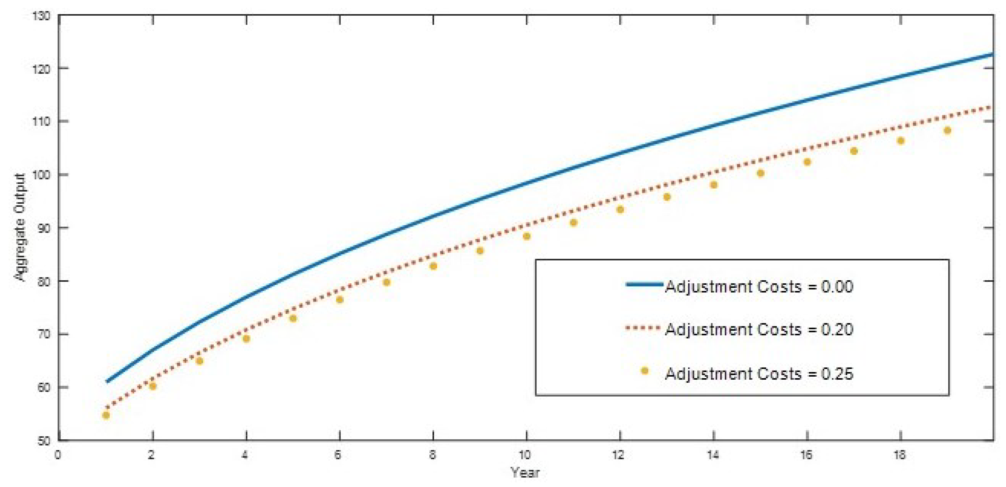
Adjustment Costs	$ϕ$	0.20	Data
Mean of Housing Shock (Impatient Agent)	$μ$ _b	0.55	Data
Standard Deviation Housing Shock (Impatient Agent)	$σ$ _b	0.05	Data
Mean of Default Shock	$μ$ _x	−0.10	Data
Standard Deviation of Default Shock	$σ$ _x	0.10	Data
Coefficient of Full Liquidity	$θ$	1.00	Assumption

Note: The main parameter values were obtained from 45 developed and developing countries between 2001 and 2022. Other parameters were obtained from Gete (2020), Quadrini (2020), and Acoling et al. (2022).

Table 2. Basic case (full liquidity).

		Interest Rates		Prices	Housing Shocks		Income		Investment		Liquidity
	Wealth	Deposits	Lending	Housing	Saver	Borrower	Saver	Borrower	Saver	Borrower	Deposits	Credits
Panel A
	W	Rd	Rl	S	e_s	e_b	Ws	Wb	m_s	m_b	d	b
$θ$ = 1; e = 1; nw = 0; gA = 0.01
Mean	159.71	1.02	1.13	1.35	0.88	1.23	66.63	53.63	2.95	31.30	38.10	45.29
Std Deviation	30.26	0.07	0.08	0.10	0.04	0.05	18.39	20.43	10.98	14.85	16.33	14.69
Rate of Growth	1.2%	0.4%	0.4%	0.6%
	W	Rd	Rl	S	e_s	e_b	Ws	Wb	m_s	m_b	d	b
$θ$ = 1; e = 1; nw = 0; gA = 0.03
Mean	168.81	1.04	1.16	1.32	0.88	1.23	53.07	62.59	0.83	31.10	20.67	29.60
Std Deviation	48.07	0.07	0.08	0.09	0.03	0.05	34.73	48.68	4.72	26.07	17.80	13.38
Rate of Growth	4.3%	0.4%	0.3%	0.7%
Panel B
	W	Rd	Rl	S	e_s	e_b	Ws	Wb	m_s	m_b	d	b
$θ$ = 1; e = 1; nw = 10; gA = 0.01
Mean	169.78	1.02	1.14	1.56	1.11	1.23	70.90	53.39	35.46	24.33	5.64	16.08
Std Deviation	32.05	0.07	0.07	0.11	0.05	0.05	18.14	16.63	17.40	10.96	15.09	13.58
Rate of Growth	1.2%	0.5%	0.5%	0.8%
	W	Rd	Rl	S	e_s	e_b	Ws	Wb	m_s	m_b	d	b
$θ$ = 1; e = 1; nw = 10; gA = 0.03
Mean	173.82	1.01	1.13	1.57	1.11	1.23	74.66	40.77	39.45	13.60	3.12	12.81
Std Deviation	36.78	0.06	0.07	0.10	0.04	0.05	30.39	23.22	19.73	9.19	11.77	10.59
Rate of Growth	2.9%	0.4%	0.4%	0.6%

Note: Table 2 shows the results we obtained by solving the model with discount factors 0.97 and 0.85, for the patient and the impatient households, respectively. In addition, agents differed in the values of the housing shocks. In panel A, we assumed zero banks’ capitalization (nw =

0

) and no intervention. In panel B, banks’ capitalization was larger than zero (nw =

10

). In both cases, we compared a productivity growth of 1% with 3%.

Table 3. Case 1 (closed economy).

		Interest Rates		Prices	Housing Shocks		Agents’ Income		Agents’ Investment		Liquidity
	Wealth	Deposits	Lending	Housing	Saver	Borrower	Saver	Borrower	Saver	Borrower	Deposits	Credits
Panel A
	W	Rd	Rl	S	e_s	e_b	Ws	Wb	m_s	m_b	d	b
$θ$ = 0.51; e = 1; nw = 0; gA = 0.01
Mean	152.02	1.02	1.13	1.56	1.11	1.23	60.04	47.64	29.03	20.88	4.63	9.82
Std Deviation	29.15	0.06	0.07	0.11	0.05	0.05	16.46	14.59	15.36	9.73	12.38	11.12
Rate of Growth	1.0%	0.3%	0.3%	0.7%
Panel B
	W	Rd	Rl	S	e_s	e_b	Ws	Wb	m_s	m_b	d	b
$θ$ = 0.51, e = 2; nw = 0; z = 0.07; gA = 0.01
Mean	153.55	1.03	1.11	1.58	1.14	1.23	58.47	50.56	28.97	24.03	2.08	13.03
Std Deviation	29.87	0.06	0.07	0.11	0.05	0.05	15.80	14.50	12.08	8.75	8.16	10.30
Rate of Growth	1.1%	0.4%	0.4%	0.5%
Panel C
	W	Rd	Rl	S	e_s	e_b	Ws	Wb	m_s	m_b	d	b
$θ$ = 0.51, e = 2; nw = 0; z = 0.07; gA = 0.03
Mean	157.48	1.02	1.09	1.60	1.14	1.23	62.90	54.46	32.43	26.20	1.14	12.06
Std Deviation	34.13	0.07	0.07	0.12	0.05	0.05	24.89	21.08	15.36	10.64	7.09	9.47
Rate of Growth	1.9%	0.5%	0.5%	0.5%

Note: Table 3 shows the results we obtained by solving the model with discount factors 0.97 and 0.85, for the patient and the impatient households, respectively. In addition, agents differed in the values of the housing shocks. In panel A, we assumed zero banks’ capitalization (nw = 0) and no intervention. In panel B, we assumed an exchange rate devaluation and a reserve ratio z = 0.07. Panel C differs from panel B by considering a rate of productivity growth of 0.03.

Table 4. Case 2 (shock on foreign liquidity).

		Interest Rates		Prices	Housing Shocks		Agents’ Income		Agents’ Investment		Liquidity
	Wealth	Deposits	Lending	Housing	Saver	Borrower	Saver	Borrower	Saver	Borrower	Deposits	Credits
Panel A
	W	Rd	Rl	S	e_s	e_b	Ws	Wb	m_s	m_b	d	b
q = 0.51; e = 1; nw = 0; gA = 0.01
Mean	152.02	1.02	1.13	1.56	1.11	1.23	60.04	47.64	29.03	20.88	4.63	9.82
Std Deviation	29.15	0.06	0.07	0.11	0.05	0.05	16.46	14.59	15.36	9.73	12.38	11.12
Rate of Growth	1.0%	0.3%	0.3%	0.7%
Panel B
	W	Rd	Rl	S	e_s	e_b	Ws	Wb	m_s	m_b	d	b
q = 0.51, e = 2; nw = 0; z = 0.07; gA = 0.01
Mean	153.55	1.03	1.11	1.58	1.14	1.23	58.47	50.56	28.97	24.03	2.08	13.03
Std Deviation	29.87	0.06	0.07	0.11	0.05	0.05	15.80	14.50	12.08	8.75	8.16	10.30
Rate of Growth	1.1%	0.4%	0.4%	0.5%
Panel C
	W	Rd	Rl	S	e_s	e_b	Ws	Wb	m_s	m_b	d	b
q = 0.51, e = 2; nw = 0; z = 0.07; gA = 0.03
Mean	157.48	1.02	1.09	1.60	1.14	1.23	62.90	54.46	32.43	26.20	1.14	12.06
Std Deviation	34.13	0.07	0.07	0.12	0.05	0.05	24.89	21.08	15.36	10.64	7.09	9.47
Rate of Growth	1.9%	0.5%	0.5%	0.5%

Note: Table 4 shows the results we obtained by solving the model with discount factors 0.97 and 0.85, for the patient and the impatient households, respectively. In addition, the economy faced a foreign liquidity shock and agents differed in the values of the housing shocks. In panel A, we assumed zero banks’ capitalization (nw = 0) and no intervention. In panel B, we assumed an exchange rate devaluation and a reserve ratio z = 0.07. Panel C differs from panel B by considering a rate of productivity growth of 0.03.

Table 5. Case 3 (perfect foreign liquidity).

		Interest Rates		Prices	Housing Shocks		Agents’ Income		Agents’ Investment		Liquidity
	Wealth	Deposits	Lending	Housing	Saver	Borrower	Saver	Borrower	Saver	Borrower	Deposits	Credits
Panel A
	W	Rd	Rl	S	e_s	e_b	Ws	Wb	m_s	m_b	d	b
$θ$ = 1; e = 1; gA = 0.01
Mean	142.12	1.20	1.33	1.33	1.11	1.23	50.26	25.70	4.64	2.55	18.08	27.27
Std Deviation	25.91	0.09	0.10	0.11	0.05	0.05	9.59	7.54	9.22	4.99	10.08	9.07
Rate of Growth	0.9%	0.8%	0.8%	0.5%
Panel B
	W	Rd	Rl	S	e_s	e_b	Ws	Wb	m_s	m_b	d	b
$θ$ = 1; e = 1; z = 0.03; gA = 0.01
Mean	144.65	1.21	1.25	1.39	1.19	1.23	50.92	28.22	9.76	5.16	12.97	23.58
Std Deviation	27.18	0.09	0.09	0.10	0.04	0.04	9.39	9.06	11.75	6.12	11.61	11.26
Rate of Growth	0.9%	0.7%	0.7%	0.4%
Panel C
	W	Rd	Rl	S	e_s	e_b	Ws	Wb	m_s	m_b	d	b
$θ$ = 1, e = 1; z = 0.03; gA = 0.03
Mean	145.72	1.19	1.23	1.41	1.19	1.23	50.71	29.31	11.53	6.18	11.21	21.87
Std Deviation	31.21	0.09	0.09	0.12	0.05	0.05	15.15	14.53	12.49	7.23	11.67	11.32
Rate of Growth	2.0%	0.7%	0.7%	0.7%

Note: Table 5 shows the results we obtained by solving the model with discount factors 0.97 and 0.85, for the patient and the impatient households, respectively. In addition, there was full foreign liquidity, and agents differed in the values of the housing shocks. In panel A, we assumed zero banks’ capitalization (nw = 0) and no intervention. In panel B, we assumed a reserve ratio z = 0.03. Panel C differs from panel B by considering a rate of productivity growth of 0.03.

Table 6. Case 4 (shock on foreign liquidity).

		Interest Rates		Prices	Housing Shocks		Agents’ Income		Agents’ Investment		Liquidity
	Wealth	Deposits	Lending	Housing	Saver	Borrower	Saver	Borrower	Saver	Borrower	Deposits	Credits
Panel A
	W	Rd	Rl	S	e_s	e_b	Ws	Wb	m_s	m_b	d	b
q = 0.5; e = 1; gA = 0.01
Mean	142.73	1.20	1.33	1.34	1.11	1.24	50.45	26.14	5.14	2.65	17.63	21.83
Std Deviation	26.43	0.09	0.10	0.11	0.05	0.05	10.16	7.83	9.57	4.89	10.47	9.72
Rate of Growth	0.9%	0.9%	0.9%	0.7%
Panel B
	W	Rd	Rl	S	e_s	e_b	Ws	Wb	m_s	m_b	d	b
q = 0.54; e = 3; z = 0.03; gA = 0.01
Mean	144.34	1.21	1.24	1.39	1.19	1.22	50.58	27.99	9.44	5.39	13.21	29.87
Std Deviation	27.62	0.08	0.08	0.10	0.05	0.05	10.48	10.32	11.66	6.79	11.64	15.09
Rate of Growth	1.0%	0.7%	0.6%	0.6%					j
Panel C
	W	Rd	Rl	S	e_s	e_b	Ws	Wb	ms	m_b	d1	b
q = 0.47, e = 3; z = 0.03; gA = 0.03
Mean	150.18	1.20	1.24	1.39	1.19	1.23	53.11	30.66	11.32	6.43	12.35	27.19
Std Deviation	32.92	0.08	0.08	0.10	0.05	0.05	15.12	16.13	12.89	8.16	12.28	15.71
Rate of Growth	1.6%	0.7%	0.7%	0.5%

Note: Table 6 shows the results we obtained by solving the model with discount factors 0.97 and 0.85, for the patient and the impatient households, respectively. In addition, there was a shock on foreign liquidity, and agents differed in the values of the housing shocks. In panel A, we assumed zero banks’ capitalization (nw = 0) and no intervention. In panel B, we assumed a currency devaluation and a reserve ratio z = 0.03. Panel C differs from panel B by considering a rate of productivity growth of 0.03.

Disclaimer/Publisher’s Note: The statements, opinions and data contained in all publications are solely those of the individual author(s) and contributor(s) and not of MDPI and/or the editor(s). MDPI and/or the editor(s) disclaim responsibility for any injury to people or property resulting from any ideas, methods, instructions or products referred to in the content.

© 2025 by the authors. Licensee MDPI, Basel, Switzerland. This article is an open access article distributed under the terms and conditions of the Creative Commons Attribution (CC BY) license (https://creativecommons.org/licenses/by/4.0/).

Share and Cite

MDPI and ACS Style

Farias, M.E.; Godoy, D.R. More or Less Openness? The Credit Cycle, Housing, and Policy. Economies 2025, 13, 207. https://doi.org/10.3390/economies13070207

AMA Style

Farias ME, Godoy DR. More or Less Openness? The Credit Cycle, Housing, and Policy. Economies. 2025; 13(7):207. https://doi.org/10.3390/economies13070207

Chicago/Turabian Style

Farias, Maria Elisa, and David R. Godoy. 2025. "More or Less Openness? The Credit Cycle, Housing, and Policy" Economies 13, no. 7: 207. https://doi.org/10.3390/economies13070207

APA Style

Farias, M. E., & Godoy, D. R. (2025). More or Less Openness? The Credit Cycle, Housing, and Policy. Economies, 13(7), 207. https://doi.org/10.3390/economies13070207

Note that from the first issue of 2016, this journal uses article numbers instead of page numbers. See further details here.

Article Menu

More or Less Openness? The Credit Cycle, Housing, and Policy

Abstract

1. Introduction

2. Related Literature

3. The Model

3.1. Households

3.2. Firms

3.2.1. The Production of Final Goods

The Demand of Consumption Goods

The Phillips Curve

3.2.2. Intermediate Production—Reproducible Capital

Rental Capital

Capital Production

3.2.3. Housing Production

3.3. Intermediaries (Banks)

3.4. Market-Clearing Conditions

3.4.1. Labor Market

3.4.2. Physical Capital Market

3.4.3. Housing Market

3.4.4. Lending

3.4.5. Final Output

3.5. The Credit Cycle

3.5.1. Credit Constraint

3.5.2. Credit Expansion

4. Monetary Policy and the Credit Cycle

4.1. Perfect Competition

4.1.1. Perfect Foresight

4.1.2. Imperfect Foresight

4.2. Cournot Competition

4.2.1. Perfect Foresight

4.2.2. Imperfect Foresight

4.3. Monetary Policy

5. Numerical Analysis

6. Conclusions

Author Contributions

Funding

Data Availability Statement

Acknowledgments

Conflicts of Interest

Appendix A. Proofs

Appendix A.1. The Phillips Curve

Appendix A.2. Rental Capital

Appendix A.3. Interest Rates

Notes

References

Share and Cite

Article Metrics

Article Access Statistics

Further Information

Guidelines

MDPI Initiatives

Follow MDPI