Abstract
We use house prices (HP) and house price indices (HPI) as a proxy to income distribution. Specifically, we analyze distribution of sale prices in the 1970–2010 window of over 116,000 single-family homes in Hamilton County, Ohio, including Cincinnati metro area of about 2.2 million people. We also analyze distributions of HPI, published by Federal Housing Finance Agency (FHFA), for nearly 18,000 US ZIP codes that cover a period of over 40 years starting in 1980’s. If HP can be viewed as a first derivative of income, HPI can be viewed as its second derivative. We use generalized beta (GB) family of functions to fit distributions of HP and HPI since GB naturally arises from the models of economic exchange described by stochastic differential equations. Our main finding is that HP and multi-year HPI exhibit a negative Dragon King (nDK) behavior, wherein power-law distribution tail gives way to an abrupt decay to a finite upper limit value, which is similar to our recent findings for realized volatility of S&P500 index in the US stock market. This type of tail behavior is best fitted by a modified GB (mGB) distribution. Tails of single-year HPI appear to show more consistency with power-law behavior, which is better described by a GB Prime (GB2) distribution. We supplement full distribution fits by mGB and GB2 with direct linear fits (LF) of the tails. Our numerical procedure relies on evaluation of confidence intervals (CI) of the fits, as well as of p-values that give the likelihood that data come from the fitted distributions.
1. Introduction
Income distributions have a long history of being modeled by the Generalized Beta (GB) family of distributions. A comprehensive summary can be found in Chotikapanich (2008), and specifically in McDonald (2008), while more recent works include Chotikapanich et al. (2018) and Dashti Moghaddam et al. (2020). The motivation for this study was to glean insight into whether income distributions exhibit power-law (“fat”) tails or display outliers such as Dragon Kings (DK) or negative Dragon Kings (nDK) Sornette and Ouillon (2012); Wheatley and Sornette (2015); Liu and Serota (2023a, 2023b). Given that identifying fat tails and outliers requires vary large datasets, available coarse-grained income data is not sufficient for this purpose. In this regard, house prices (HP) may serve as a proxy to—or “derivative” of—incomes.
Previously, we considered sale prices of houses in Hamilton County, Ohio from 1970 to 2010 in the context of analysis of inequality indices Dashti Moghaddam et al. (2020). Here we pare down that data to include only single-family homes, which better aligns to incomes, as well as to house price indices (HPI), which are also based on single-family HP and are constructed using repeat-sale methodology Bailey et al. (1963), Case and Shiller (1987, 1989), Calhoun (1996), Bogin et al. (2016). Specifically, we utilize FHFA HPI for nearly 18,000 US ZIP codes over a period of 40 years, starting in 1980’s Bogin et al. (2016). HPI can be viewed as a proxy to HP—or a “second derivative” of income distribution—in this case between different ZIP codes.
Our approach to analyzing HP and HPI distributions mirrors the approach we used for analysis of the distributions of historical realized volatility Liu and Serota (2023a). Namely, we fitted the entire distribution with modified Generalized Beta (mGB) and Generalized Beta Prime (GB2) distributions, as well as performed a linear fit (LF) of the tails. For each fit, we evaluated confidence interval (CI) as well as conducted a U-test Liu and Serota (2023a), Pisarenko and Sornette (2012), which yields p-values that indicate the likelihood of the data coming from the fitted distribution.
Since fat tails are scale free, they are naturally analyzed on a log-log scale, where complementary cumulative distribution function (CCDF) ought to be a straight line with negative slope. LF of CCDF, however, must be supplemented by a statistical test to determine the likelihood that the points in the tail conform to linearity or whether outliers may be present Wheatley and Sornette (2015). In this case we are concerned with possibility of observing DK, where the ends of the tails shoot upward from LF, or nDK, where tails’ ends shoot down.
Towards this end, we performed a U-test Pisarenko and Sornette (2012) but we did not limit it to LF alone. We also aimed at describing the entire distribution, not just tails, and thus performed a U-test on mGB and GB2, which we employed for this purpose. GB2 was used for fitting since it is the most flexible distribution with fat tails and mGB, while exhibiting similar tails over a wide range of variable, abruptly terminates at finite value, which seems appropriate to describe nDK behavior Liu and Serota (2023b). Of particular importance is the fact that both mGB and GB2 arise as steady-state (stationary) distributions of stochastic differential equations that mean to serve as models of economic exchange Bouchaud and Mézard (2000); Dashti Moghaddam et al. (2020); Ma et al. (2013).
This paper is organized as follows. In Section 2 we present the analytical form of mGB and GB2 distributions and discuss the limiting behaviors of both. In Section 3 we fit HP and HPI with mGB and GB 2, as well as the fit tails directly using LF. For each test we conduct a U-test, for which a null hypothesis is formulated, and plot p-values which reflect on the goodness of fit, as well as whether DK or nDK behavior may be present. We conclude in Section 4 with discussion of our results.
2. Generalized Beta Distribution Function
A detailed discussion of the Modified Generalized Beta (mGB) distribution function, used here to fit the distributions of HP and HPI, as well as of the Generalized Beta (GB) family of distributions in general, can be found in Liu and Serota (2023a, 2023b). A generalization of the traditional GB distribution McDonald and Xu (1996) can be written (in a slightly modified form relative to that of Liu and Serota (2023b)) as follows Liu and Serota (2023a):
where and are scale parameters and , p and q are shape parameters, all positive, is the beta function and . Although it has a concise and transparent form, it does not come out as a solution of a stochastic differential equation (SDE) Hertzler (2003), the latter being desirable for the purpose of modeling behavior of quantities, such as stochastic volatility, important for understanding of implied and realized volatility in equity markets Dashti Moghaddam and Serota (2021), and income distribution, resulting from economic exchange Bouchaud and Mézard (2000); Dashti Moghaddam et al. (2020); Ma et al. (2013).
The probability density function (PDF) of mGB, which comes out as a solution of an SDE (with minor caveats explained in Liu and Serota (2023b)) and which is used here to model HP and HPI distributions, can be written as
where and are scale parameters and , p and q are shape parameters, all positive, is the beta function and . The cumulative distribution function (CDF) and complementary CDF (CCDF) of mGB are given respectively by
and
where the first term in (3) and (4) represent, respectively, CDF and CCDF of GB (whose PDF is given by (1)), while and are, respectively, the regularized and incomplete beta functions NIST (2022).
In what follows, we will be specifically interested in the circumstance since for GB and mGB exhibit a power-law dependence,
In the limit of , mGB and GB become, respectively, mGB2 and GB2 (the latter also known as Generalized Beta Prime) and are given by Liu and Serota (2023b)
and
Unlike mGB and GB, for whom the power-law dependences in (5) eventually terminate at , mGB2 and GB2 will sustain these power-law dependences indefinitely.
Below, we will use (4) to fit CCDF of distributions of HP and HPI. As explained in Liu and Serota (2023b), mGB2 and GB2 are equivalent since q and p are independently defined at this level of GB family of distributions, and q can be shifted by unity in the definition of mGB2/GB2. Consequently, we choose a more familiar CCDF of GB2
to fit CCDF of the HP and HPI data. Insofar as the main difference between mGB and GB is concerned, it is their behavior near in the present context Liu and Serota (2023b). Namely,
and
that is drops off to zero ( saturates to unity) faster than due to the factor . This feature accounts for a better fit via mGB versus GB, which may be due to the fact that mGB emerges from a physically motivated stochastic model Liu and Serota (2023b).
3. Fitting Distribution of House Prices and House Price Indices
3.1. Methodology
Our analysis of HP and HPI distributions mirrors that of our analysis of distributions of realized volatility in Liu and Serota (2023a). Namely, we perform Bayesian fitting of the entire distributions of HP and HPI using mGB, as per (2)–(4), and GB2, as per (7) and (8). We also perform LF of the tails. Confidence intervals (CI) for the fits are evaluated via inversion of the binomial distribution Janczura and Weron (2012); p-values are evaluated in the framework of the U-test, which is based on order statistics Pisarenko and Sornette (2012), using the following formula:
where is the k’s member of numbers between 1 and m ordered by increasing magnitude (HP and HPI in this case), and is the assumed CDF (mGB, GB2 and LF here). p-values are evaluated in order to test the null hypothesis : all observations of the sample are generated by the same fitting distribution. The p-value (11) is defined as a probability of exceeding the observed value under the null hypothesis. If among the p-values there are some small values—≤0.05 here—then those observed values are identified as DK with probability . Conversely, large p-values—≥0.95 here—are identified as nDK with the probability p Pisarenko and Sornette (2012).
For each of the distributions we organize figures as follows:
- PDF of the distribution
- Full data CDF fit with mGB and GB2 and LF of the tails;
- Same as above but showing specifically the tail region;
- p-values of all three fits in the tail region, with indicating DK (up triangles) and nDK (down triangles);
- LF with its CI;
- GB2 fit with its CI;
- mGB fit with its CI.
3.2. Distribution of House Prices
In this section we fit the distribution of sale prices of single-family homes in Hamilton County, Ohio between 1970 and 2010. This dataset contains 116,207 entries and sale prices are converted to constant dollars to eliminate the effect of inflation. Table 1 gives all estimated parameters of mGB and GB2 distributions and slopes of two linear fits: LF-1 is performed by visually excluding possible outliers Pisarenko and Sornette (2012) and LF-2 by excluding HP whose sale price was above 90% of the top HP.

Table 1.
All estimated parameters of mGB and GB2 fits of HP distribution and slopes of GB2 and of LFs.
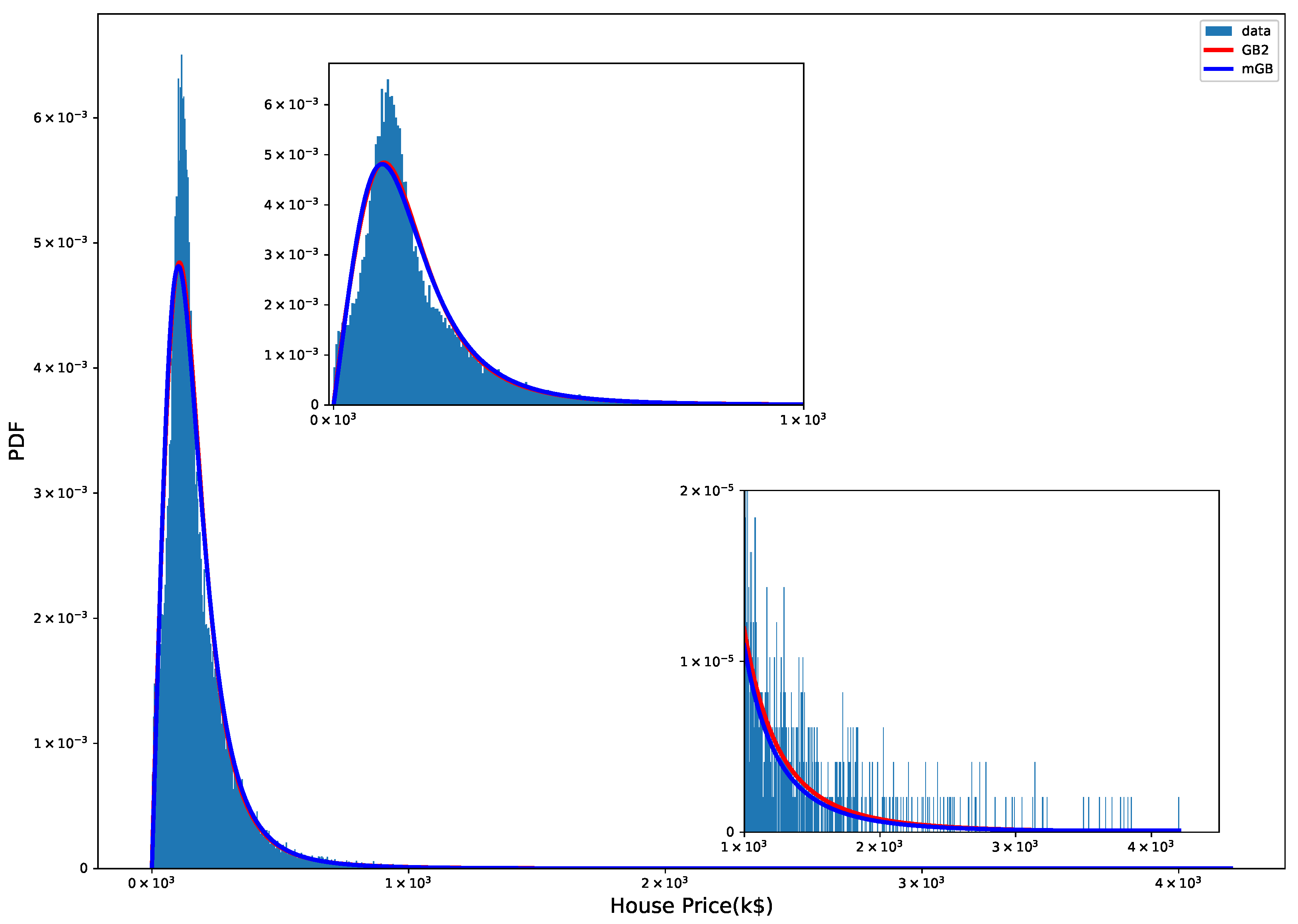
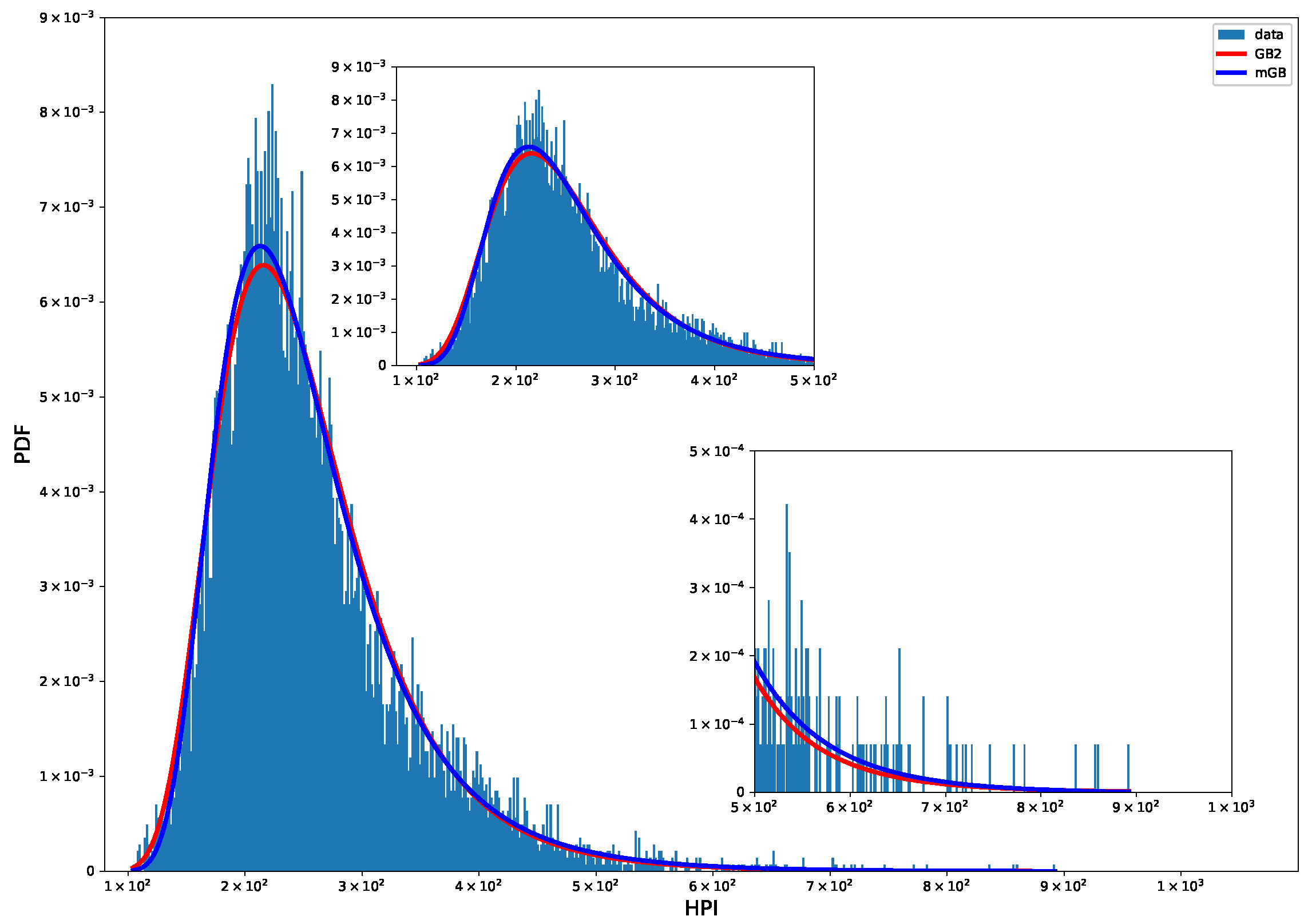
Figure 1 shows probability density function (PDF) of HP with mGB and GB2 fits. Clearly neither fit does a good job for typical values HP.
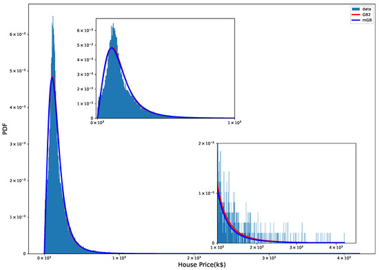
Figure 1.
HP PDF: mGB and GB2 fits.
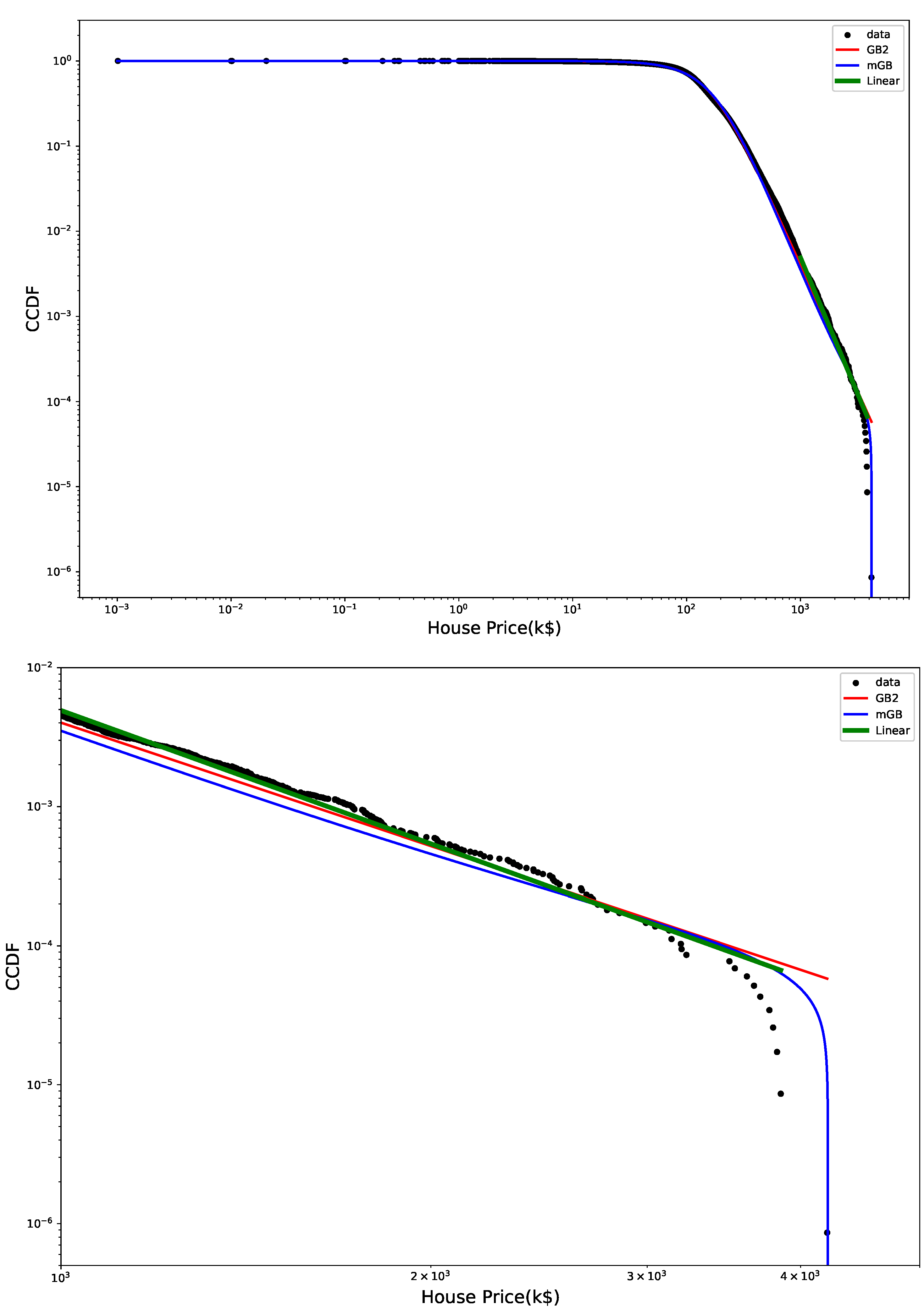
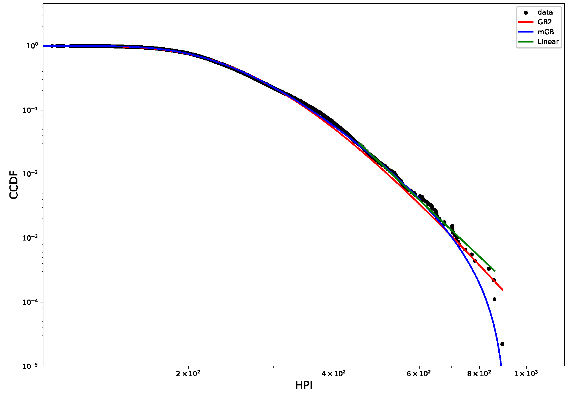
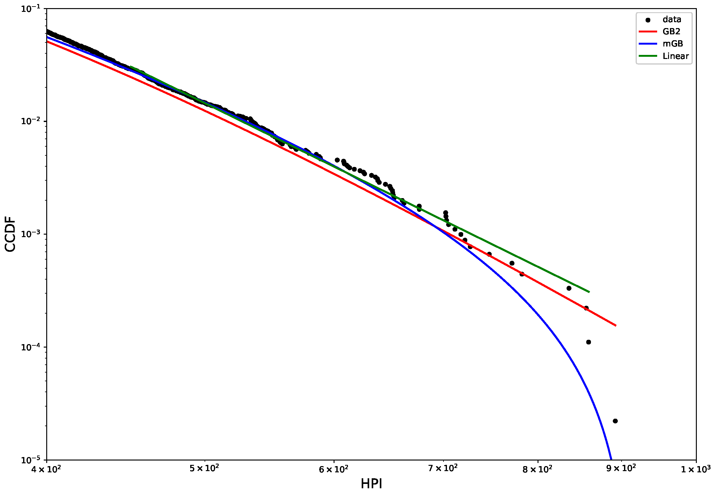
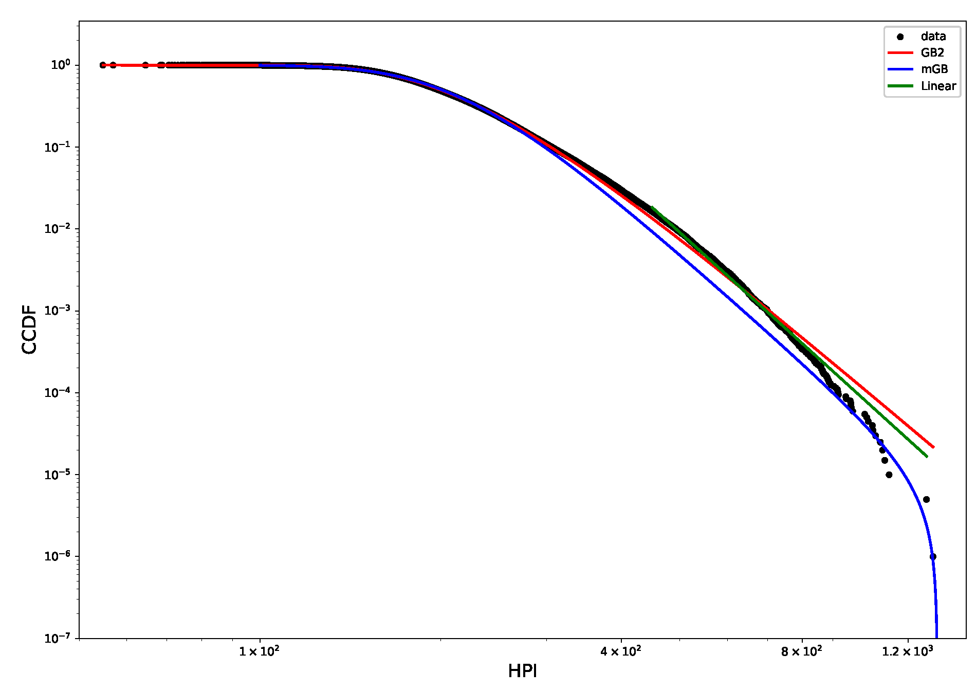
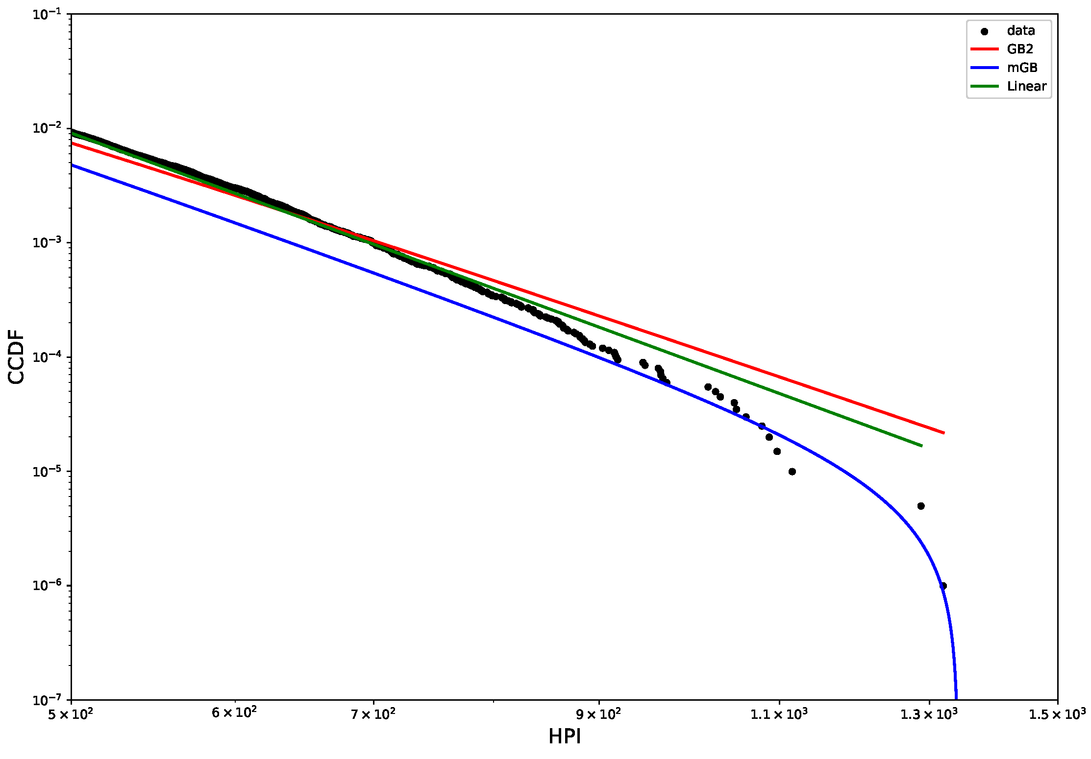
Figure 2 shows CCDF of the HP distribution on a log-log scale, with its mGB and GB2 fits and LF of the tail. The tail area is further expanded for a better view. Clearly the end points of the tail fall off abruptly from what looks like a rather well-defined power-law dependence, prompting a possibility that they may considered nDK.
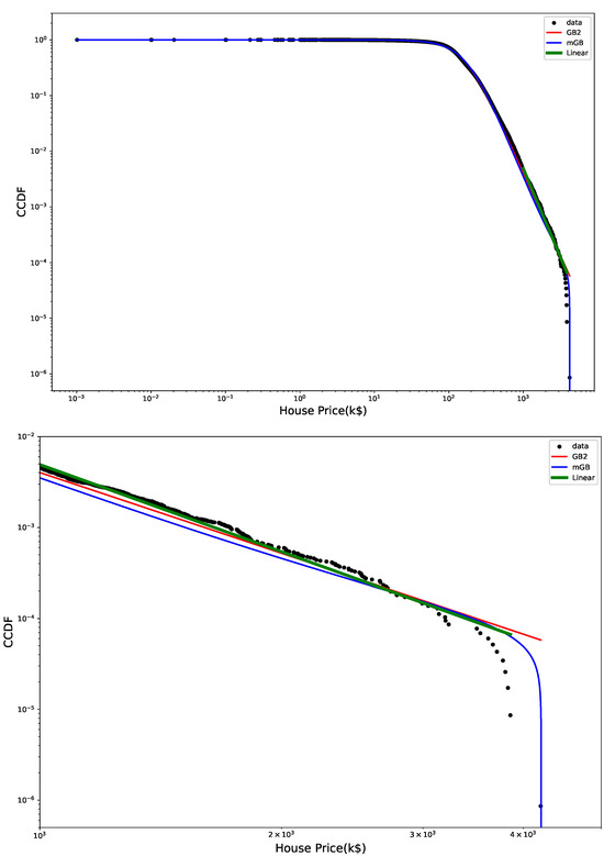
Figure 2.
HP CCDF: mGB, GB2 fits of the full distribution and LF of the tail (top); tail area (bottom).
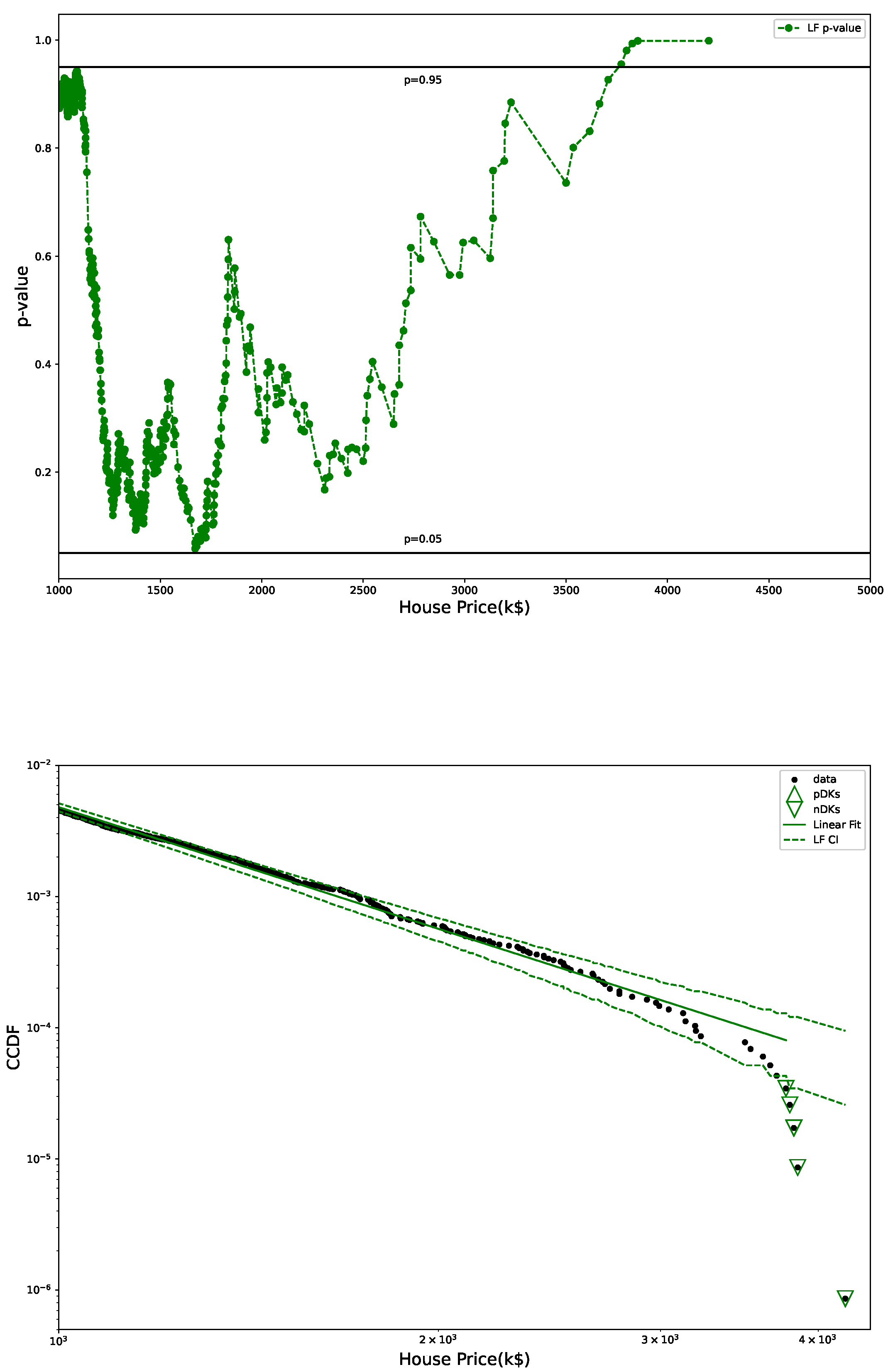
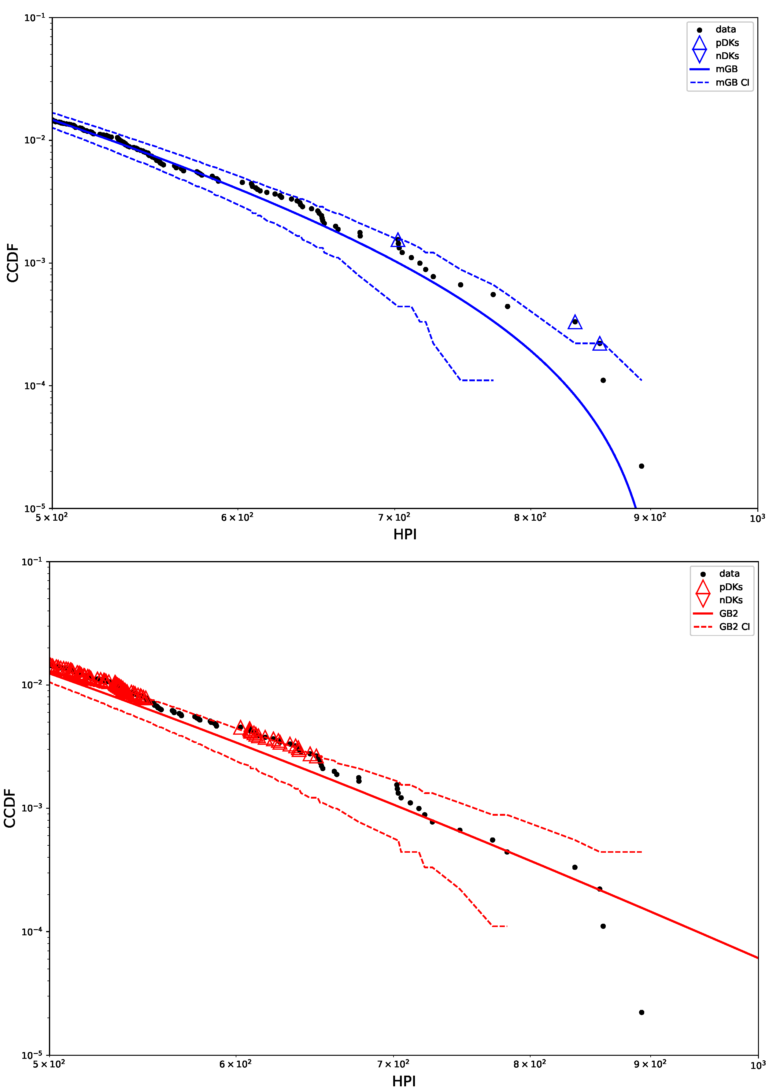
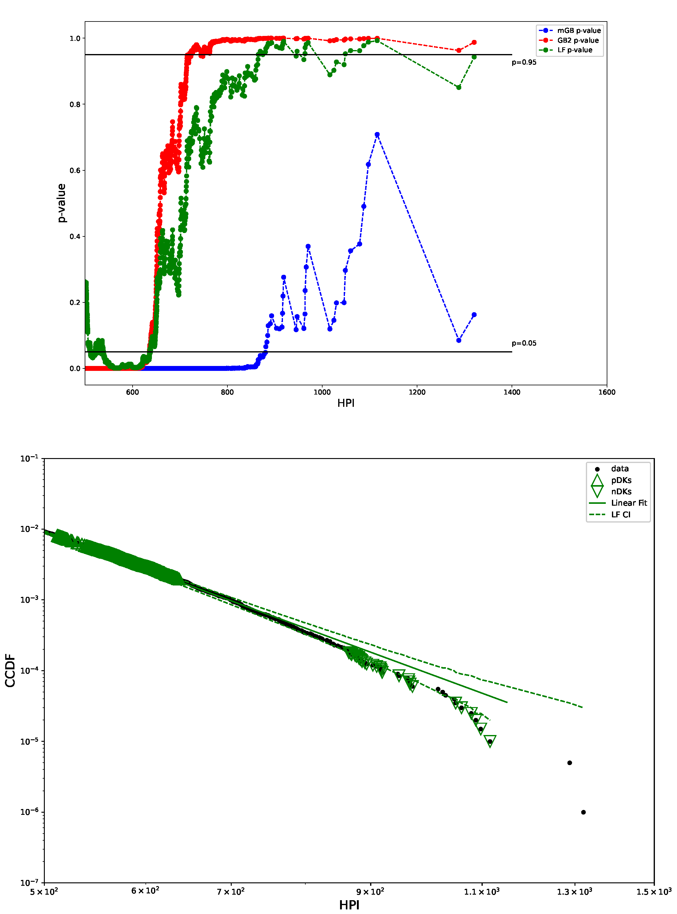
Figure 3 shows p-values obtained in U-test for all three fits (mGB, GB2 and LF), as well as the LF with its CI (dashed line). p-values such that , had they been at the tail ends, could be considered DK, however in the earlier parts of the tail they are merely an indication of a poor fit (as are values ). We dubbed them “potential DK” (pDK) and mark in the plot with up triangles. p-values at the tail ends may qualify as actual nDK.
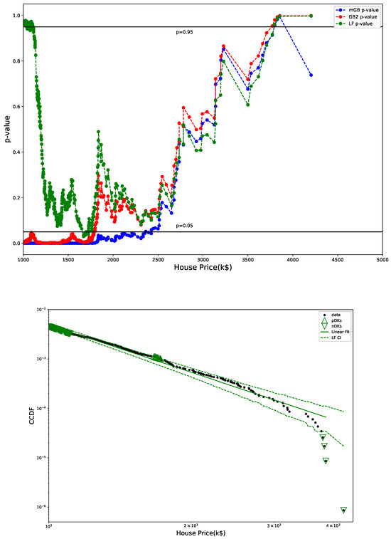
Figure 3.
p-values from U test (top) and LF with CI (bottom): CI marked by dashed lines, pDK by up triangles, nDK by down triangles; LF excludes points visually deemed as possible nDK.
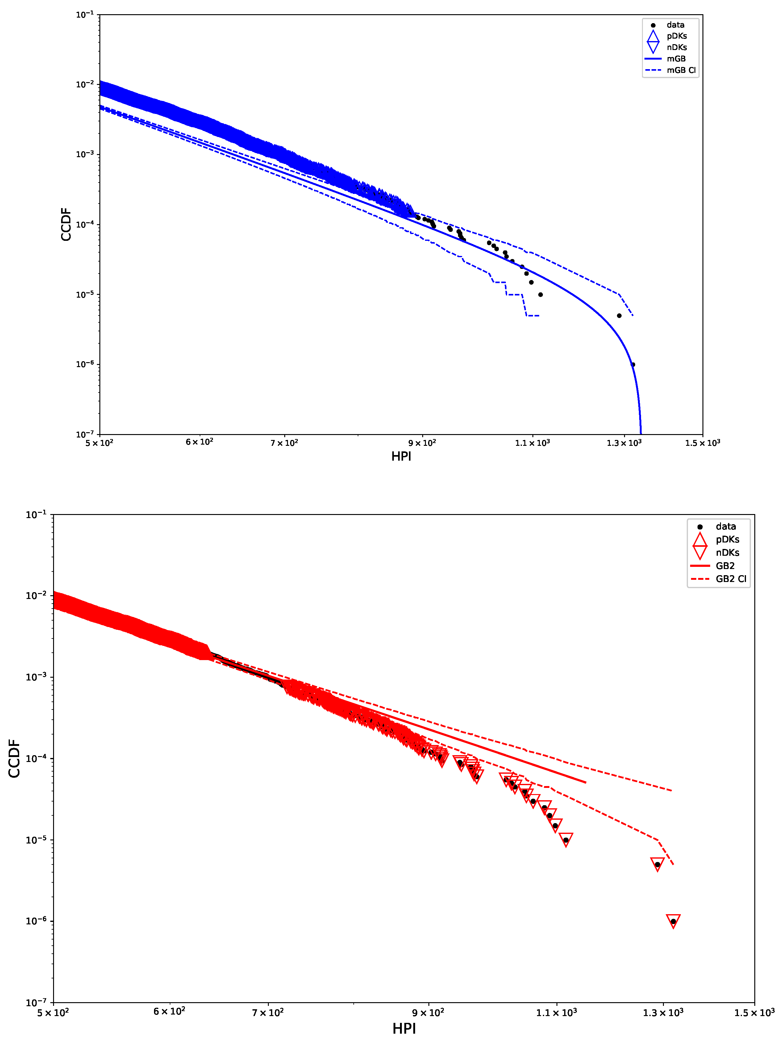
Figure 4 shows tail areas of mGB and GB2 fits, with their CI, pDK, and nDK. Clearly mGB makes a decent attempt at approximating nDK behavior. However, earlier part of the tail (as well as full PDF above) indicate a rather poor fit by either.
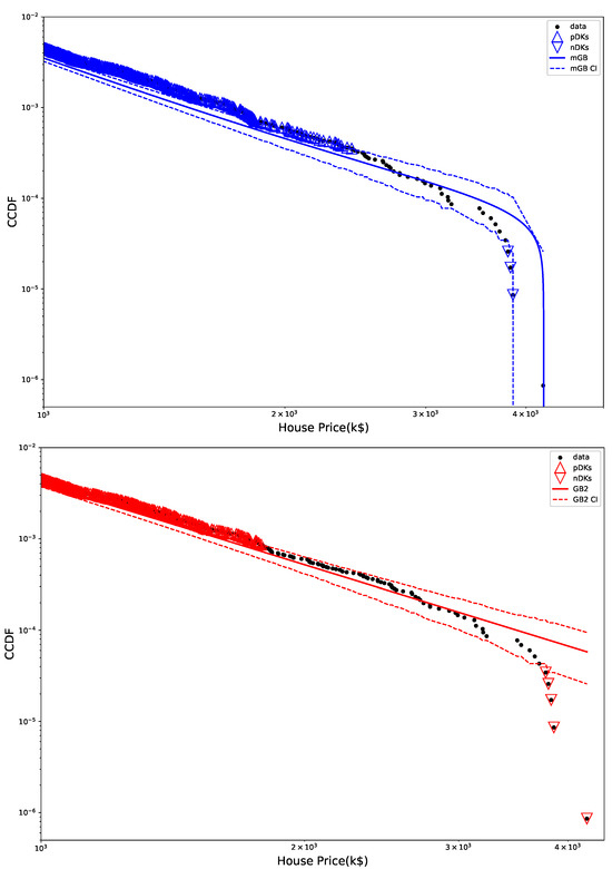
Figure 4.
mGB fit with CI (top) and GB2 fit with CI (bottom) shown for tail area: CI marked by dashed lines, pDK by up triangles, nDK by down triangles.
Figure 5 shows p-value plot and LF, whose main difference from Figure 3 is that LF is done by excluding the end points with HP greater than 90% of the top price, rather than excluding possible outliers (nDK here) visually. Clearly, there is essentially very little difference between the two. It is the case for HPI as well, so we do not present a corresponding plot for HPI below.
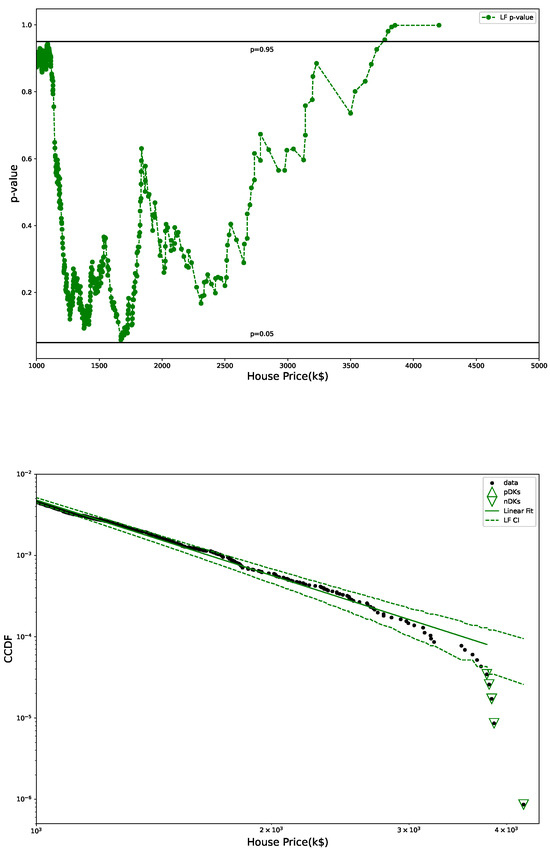
Figure 5.
p-values from U test (top) and LF with CI (bottom): CI marked by dashed lines, pDK by up triangles, nDK by down triangles; LF excludes points with HP above 90% of top HP.
3.3. Distribution of House Price Indicies
HPI are constructed using repeat-sale methodology Bailey et al. (1963), Case and Shiller (1987, 1989), Calhoun (1996), Bogin et al. (2016). Specifically, we utilize FHFA HPI for nearly 18,000 US ZIP codes over a period of 40 years, starting in 1980’s Bogin et al. (2016). HPI are updated annually on FHFA site FHFA (2024). HPI can be viewed as a proxy to HP, which in turn can be viewed as a proxy to income distribution—here between different ZIP codes. In what follows, we initially analyze single-year distributions of HPI, followed by the multi-year distribution, which can be considered as a sum of single-year distributions.
3.3.1. Single-Year Distribuions
We conducted fitting and analysis of a number of single-year HPI and found the results to be very similar, in particular over last two decades. Therefore here we present the results for only one year, 2019. The dataset contains HPI for 9033 zip codes. Table 2 contains all parameters of the fits, as well as slopes of GB2 and LF.
Table 2.
All estimated parameters of mGB and GB2 fits of 2019 HPI distribution and slopes of GB2 and of LF.
Figure 6 shows PDF of single-year HPI with mGB and GB2 fits. Visually these PDF fits are considerably better than those of HP.

Figure 6.
HPI 2019 PDF: mGB and GB2 fits.
Figure 7 shows CCDF of the HPI distribution on a log-log scale, with its mGB and GB2 fits and LF of the tail. The tail area is further expanded for a better view. Visually, the tail behavior is more consistent with power law than was the case of HP. This is further confirmed by p-values obtained in the U-test (see Figure 8 below).
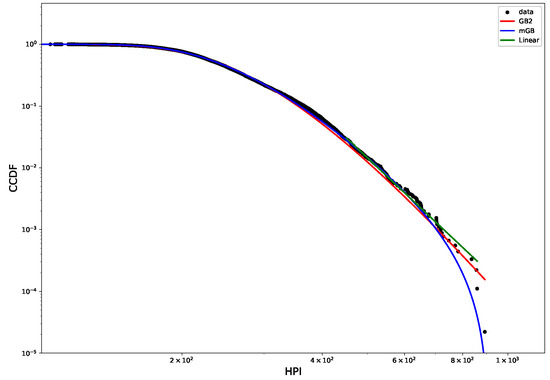
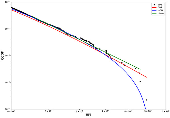
Figure 7.
HPI 2019 CCDF: mGB, GB2 fits of the full distribution and LF of the tail (top); tail area (bottom).
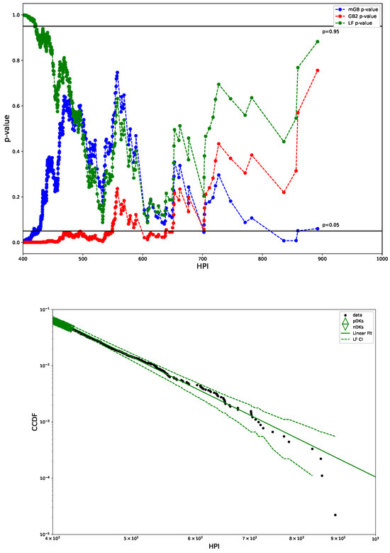
Figure 8.
p-values from U test (top) and LF with CI (bottom): CI marked by dashed lines, pDK by up triangles, nDK by down triangles; LF excludes points visually deemed as possible nDK.
Figure 8 shows p-values obtained in U-test for all three fits (mGB, GB2 and LF), as well as the LF with its CI (dashed line). We observe that GB2 and LF do not have p-values , which indicates less likelihood of outliers form the power-law behavior than was seen for HP, consistent with the previous visual observation in Figure 7.
Figure 9 shows tail areas of mGB and GB2 fits, with their CI, pDK, and nDK. Both distributions are relatively successful at approximating different parts of the tail.
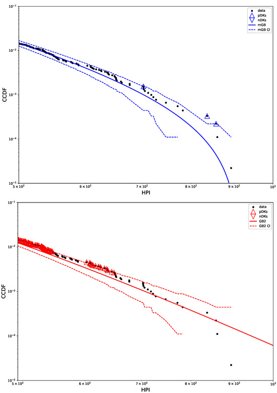
Figure 9.
mGB fit with CI (top) and GB2 fit with CI (bottom) shown for tail area: CI marked by dashed lines, pDK by up triangles, nDK by down triangles.
3.3.2. Muli-Year Distibuions
As was discussed in Section 3.3.1, tails of single-year HPI align better with power law than those of HP. However, there is also an obvious trend towards moving down from the straight line at tails ends. Since single-year HPI also have an oder of magnitude fewer points than HP, we wanted to ascertain whether this trend was significant.
Towards this end we studied a combined multi-year distribution of HPI for years 2000–2022, which contained 201,040 data points. The main result, as seen in Figures 11 and 12 below is that the tails of the combined HPI is more aligned with the finite upper limit of HPI and, accordingly, with mGB distribution. Of course, such upper limit of the variable does not have to be fixed—it may change as HPI is updated annually.
Table 3 contains all parameters of the fits of the multi-year distribution, as well as slopes of GB2 and LF.
Table 3.
All estimated parameters of mGB and GB2 fits of HPI distribution for years 2000-2022 and slopes of GB2 and of LF.
Figure 10 shows PDF of multi-year HPI with mGB and GB2 fits. Visually the fits are better than their single-year counterpart, most likely because of a much larger dataset.
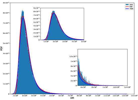
Figure 10.
HPI 2000-2022 PDF: mGB and GB2 fits.
Figure 11 shows CCDF of the multi-year HPI distribution on a log-log scale, with its mGB and GB2 fits and LF of the tail. The tail area is further expanded for a better view. Visually, the tail behavior is more consistent with finite upper limit and mGB distribution than that of a single-year HPI, and is similar to HP. This is further confirmed by p-values obtained in the U-test (see Figure 12 below).
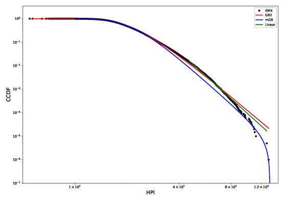
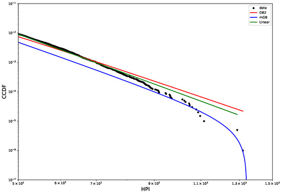
Figure 11.
HPI 2000–2022 CCDF: mGB, GB2 fits of the full distribution and LF of the tail (top); tail area (bottom).
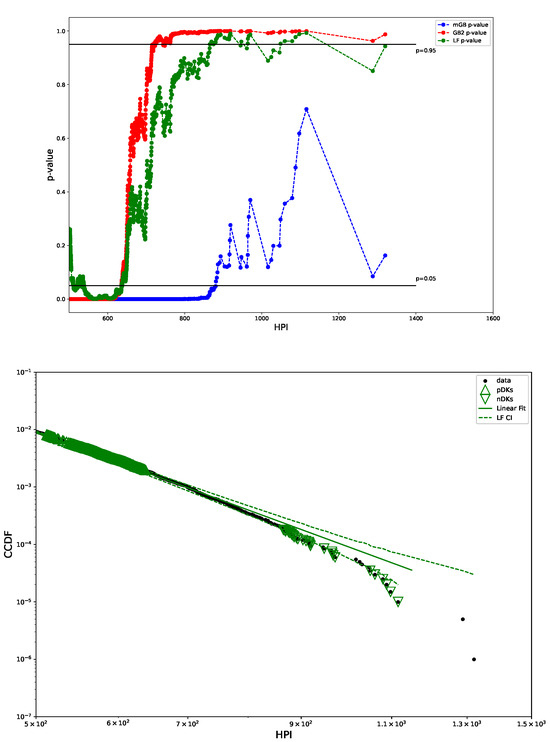
Figure 12.
p-values from U test (top) and LF with CI (bottom): CI marked by dashed lines, pDK by up triangles, nDK by down triangles; LF excludes points visually deemed as possible nDK.
Figure 12 shows p-values obtained in U-test for all three fits (mGB, GB2 and LF), as well as the LF with its CI (dashed line). We observe that, unlike GB2 and LF, mGB does not have p-values at tail ends, consistent with the previous visual observation in Figure 7. Conversely, for GB2 and for mGB indicate poor fits at the onset of the tails.
Figure 13 shows tail areas of mGB and GB2 fits, with their CI, pDK, and nDK. Clearly mGB approximates rather well nDK behavior at the tail ends, which indicates a finite upper limit. However, as indicated above, the earlier part of the tail indicate a rather poor fit by either.

Figure 13.
mGB fit with CI (top) and GB2 fit with CI (bottom) shown for tail area: CI marked by dashed lines, pDK by up triangles, nDK by down triangles.
4. Discussion
We studied distributions of house prices and house price indices. The key question we attempted to answer is whether those distributions have power-law (fat) tails or they are characterized by outliers at the tails ends, such as Dragon Kings and negative Dragon Kings, which is not unlike the search for outliers and deviations from power-law scaling in financial markets Filimonov and Sornette (2015); Johansen and Sornette (2001); Liu and Serota (2023a); Watorek et al. (2021). Towards this end, we conducted a linear fit of the tails of the complementary cumulative distribution functions on the log-log scale. In doing so, we excluded potential outliers - negative Dragon Kings here - and evaluated fits’ confidence intervals, as well as conducted a U-test for the potential outliers which provides us with p-values that indicate whether they belong to the linear fit.
Except for single-year house price indices, the distributions are characterized by a sharp drop-off from the from the log-log straight CCDF line—the latter indicating a power-law dependence—at the tail ends. From a more precise analysis based on the linear fit, confidence intervals, and p-values we can conclude that house price distributions and combined multi-year house price indices exhibit negative Dragon King behavior at the tail ends. Single-year house price indices, on the other hand, are not inconsistent with linear dependence, that is with power-law tails.
Our interest to house prices and house price indices was motivated by their being proxies to income distributions. Income distributions may be possible to describe by models of economic exchange, some of which can be reduced to stochastic differential equations with well-defined steady-state distributions. One class of such models results in steady-state distributions that belong to the Generalized Beta family of distributions. Therefore we also attempted to fit the entire empirical distributions with Generalized Beta Prime and modified Generalized Beta distributions: for a particular relationship between scale parameters the former is characterized by a power-law tail, while the latter follows the same power-law dependence, which is subsequently terminated at the finite value of the variable.
We find that modified Generalized Beta has some success in describing tail ends, however it is difficult to fully access overall goodness of fit. In particular we find that using Kolmogorov-Smirnov statistic for comparing goodness of fit between GB2 and mGB is rather inconclusive. Among idiosyncrasies are the following: despite an extra scale parameter, modified Generalized Beta may have large statistic than Generalized Beta Prime; for two close values of statistic the higher one may yield a better fit of the tail1; the largest values of statistic may occur prior to the onset of the tails. While there exist Monte-Carlo techniques aimed at estimating goodness of fit, we believe that they need further development, especially for distributions with power-law tails. We hope to address these issues in a future publication. Additionally, in terms of future research, it would be interesting to extend our study to other geographical locations and to investigate correlation between actual income and wealth and the house prices and house price indices.
Author Contributions
J.L. and H.F. performed all numerical calculations, R.A.S. was a lead on analytical part and on problem statement. All authors have read and agreed to the published version of the manuscript.
Funding
This research received no external funding.
Informed Consent Statement
Not applicable.
Data Availability Statement
Our dataset of Hamilton County, Ohio house prices is available upon request. Datasets of house price indices can be found at https://www.fhfa.gov/DataTools/Downloads/Pages/House-Price-Index.aspx (accessed on 8 February 2024).
Acknowledgments
We used Wolfram Mathematica (https://www.wolfram.com/mathematica/ accessed on 12 February 2023) in a subset of analytical calculations and MathWorks Matlab (https://www.mathworks.com/?s_tid=gn_logo accessed on 12 February 2023) for much of the numerical work.
Conflicts of Interest
The authors have no conflicts of interest to declare.
Note
| 1 | In this regard, for HPI we presented mGB and GB2 with slightly higher Kolmogorov-Statistic but with better tail fits. |
References
- Bailey, Martin J., Richard F. Muth, and Hugh O. Nourse. 1963. A regression method for real estate price index construction. Journal of American Statistical Association 58: 933–42. [Google Scholar] [CrossRef]
- Bogin, Alexander N., William M. Doerne, and William D. Larson. 2016. Local House Price Dynamics: New Indices and Stylized Facts. Working Paper 16-01, Federal Housing Finance Agency. Available online: https://www.fhfa.gov/PolicyProgramsResearch/Research/Pages/wp1601.aspx (accessed on 8 February 2024).
- Bouchaud, Jean-Philippe, and Marc Mézard. 2000. Wealth condensation in a simple model of economy. Physica A: Statistical Mechanics and its Applications 282: 536–45. [Google Scholar] [CrossRef]
- Calhoun, Charles A. 1996. Ofheo House Price Indexes: Hpi Technical Description; Working Paper N508; Washington, DC: Office of Federal Housing Enterprise Oversight.
- Case, Karl E., and Robert J. Shiller. 1987. Prices of single-family homes since 1970: New indexes for four cities. New England Economic Review, 45–56. [Google Scholar]
- Case, Karl E., and Robert J. Shiller. 1989. The efficiency of the market for single-family homes. The American Economic Review 79: 125–37. [Google Scholar]
- Chotikapanich, Duangkamon, ed. 2008. Modeling Income Distributions and Lorenz Curves. Berlin/Heidelberg: Springer. [Google Scholar]
- Chotikapanich, Duangkamon, William E. Griffiths, Gholamreza Hajargasht, Wasana Karunarathne, and Prasada D. S. Rao. 2018. Using the gb2 income distribution. Econometrics 6: 21. [Google Scholar] [CrossRef]
- Dashti Moghaddam, M., Jeffrey Mills, and R. A. Serota. 2020. From a stochastic model of economic exchange to measures of inequality. Physica A 559: 125047. [Google Scholar] [CrossRef]
- Dashti Moghaddam, M., and R. A. Serota. 2021. Combined mutiplicative-heston model for stochastic volatility. Physica A: Statistical Mechanics and Its Applications 561: 125263. [Google Scholar] [CrossRef]
- FHFA. 2024. House Price Index; Washington, DC: FHFA.
- Filimonov, Vladimir, and Didier Sornette. 2015. Power law scaling and “dragon-kings” in distributions of intraday financial drawdowns. Chaos, Solitons Fractals 74: 27–45. [Google Scholar] [CrossRef]
- Hertzler, Greg. 2003. “Classical” probability distributions for stochastic dynamic models. Paper presented at 47th Annual Conference of the Australian Agricultural and Resource Economics Society, Fremantle, Australia, February 12–14. [Google Scholar]
- Janczura, J., and R. Weron. 2012. Black swans or dragon-kings? a simple test for deviations from the power law. European Physical Journal Special Topics 205: 79–93. [Google Scholar] [CrossRef]
- Johansen, Anders, and Didier Sornette. 2001. Large stock market price drawdowns are outliers. Journal of Risk 4: 69–110. [Google Scholar] [CrossRef]
- Liu, Jiong, and R. A. Serota. 2023a. Are there dragon kings in the stock market? arXiv arXiv:2307.03693. [Google Scholar]
- Liu, Jiong, and R. A. Serota. 2023b. Rethinking generalized beta family of distributions. The European Physical Journal B 96: 24. [Google Scholar] [CrossRef]
- Ma, Tao, John G. Holden, and R. A. Serota. 2013. Distribution of wealth in a network model of the economy. Physica A: Statistical Mechanics and Its Applications 392: 2434–41. [Google Scholar] [CrossRef]
- McDonald, James B. 2008. Modeling Income Distributions and Lorenz Curves. Edited by Duangkamon Chotikapanich. Berlin/Heidelberg: Springer, Chapters 3, 8. [Google Scholar]
- McDonald, James B., and Yexiao J. Xu. 1996. A generlazition of the beta distribution with applications. Journal of Econometrics 66: 133–52. [Google Scholar] [CrossRef]
- NIST Digital Library of Mathematical Functions. 2022. Available online: https://dlmf.nist.gov (accessed on 8 February 2024).
- Pisarenko, Vladilen F., and Didier Sornette. 2012. Robust statistical tests of dragon-kings beyond power law distribution. The European Physical Journal Special Topics 205: 95–115. [Google Scholar] [CrossRef]
- Sornette, Didier, and Guy Ouillon. 2012. Dragon-kings: Mechanisms, statistical methods and empirical evidence. The European Physical Journal Special Topics 205: 1–26. [Google Scholar] [CrossRef]
- Watorek, Marcin, Jaroslaw Kwapien, and Stanislaw Drozdz. 2021. Financial return distributions: Past, present, and covid-19. Entropy 23: 884. [Google Scholar] [CrossRef] [PubMed]
- Wheatley, Spencer, and Didier Sornette. 2015. Multiple Outlier Detection in Samples with Exponential & Pareto Tails: Redeeming the Inward Approach & Detecting Dragon Kings. arXiv arXiv:1507.08689. [Google Scholar]


Disclaimer/Publisher’s Note: The statements, opinions and data contained in all publications are solely those of the individual author(s) and contributor(s) and not of MDPI and/or the editor(s). MDPI and/or the editor(s) disclaim responsibility for any injury to people or property resulting from any ideas, methods, instructions or products referred to in the content. |
© 2024 by the authors. Licensee MDPI, Basel, Switzerland. This article is an open access article distributed under the terms and conditions of the Creative Commons Attribution (CC BY) license (https://creativecommons.org/licenses/by/4.0/).