The Effects of Oil Price Volatility on South African Stock Market Returns

Abstract

The aim of this study is to assess the response of the South African stock market returns to oil price volatility, based on the daily South African stock market index, using the GARCH-Copula modelling technique. The results of the analysis show evidence of an asymmetric impact of fluctuations in oil prices on South African stock market returns, using a copula model specification, particularly the bivariate symmetrized Joe-Clayton (SJC) copula. The results also revealed that the EGARCH process is the best univariate model to capture oil price volatility. Interestingly, this study also revealed that the tourism industry is most dependent on oil price fluctuations, due to its heavy reliance on transportation costs. The economic implications of this study also suggest that sectors affected by oil price fluctuations need specific long-term and short-term monetary policy strategies. It is recommended that in the short term, expansionary monetary policy could assist in mitigating the impact of higher oil prices, while in the long-term, policies aimed at reducing the volatility in oil prices would be of great help in alleviating its harmful effect on stock market returns.

1. Introduction

Energy, as one of the greatest resources of countries throughout history, has become a major topic of concern as its usage has grown in the industrial sector and contributes to economic growth. Accordingly, economic growth is closely tied to efficient policies of the supply and demand of energy. Research has shown that the consumption of energy is highly associated with economic growth (Pirlogea and Cicea 2012). All sectors of life hinge on energy; hence, the world must increase energy supply at a rate that is affordable, safe, secure, and environmentally responsible in the coming decade. The challenges are enormous and require the setting of integrated solutions. Effective long-term planning and a thorough infrastructure, coupled with years of significant investment, are essential for a successful supply and demand strategy. Oil is one of the most efficient forms of energy, and research on its price inconsistency has progressed since the oil price shocks of the 1970s. In a cause-and-effect relationship, oil price volatility and inflation levels are usually assumed to be linked. Inflation, which is a measurement of the economy’s general price trends, rises in lockstep with oil prices. As stated by OPEC (2020), as the price of oil falls, inflationary pressures would equally begin to ease. Ferdi and Yildirim (2014) also noted that because of limited supply policies, net oil-importing countries are susceptible to oil price fluctuations. This negatively impacts the economic progress of those countries and predominantly developing countries. South Africa has the largest stock market on the African continent. It is also one of the oldest in Africa. It is regarded as the gateway for investment in the rest of the African continent. The activities on the stock market in South Africa have a potential to impact the investment in the rest of the African continent.

The link between oil price shocks and stock market volatility has gotten a lot of attention, with the majority of the literature focusing on industrialized countries, notably the study by Arouri and Nguyen (2010) who investigated oil and stock market volatility spillovers, using European data. Their analysis discovered a lot of proof of volatility spillovers, with the biggest ones transferring from oil to stock markets. Surprisingly, their investigation revealed that volatility spillovers between two marketplaces are unimportant. Similarly, Choi and Hammoudeh (2010) used the VAR, Granger causality, impulse responses, and a logistic transition model to study the influence of oil price volatility in the US, UK, and India on emerging stock markets. The findings demonstrated a non-linear link between oil prices’ fluctuation and the stock market index in emerging economies.

Studies by Bouri (2015) and Silvapulle et al. (2017) established that oil-importing countries are negatively affected by oil price changes. Accordingly, studies related to oil price volatility are crucial for developing policy strategy in South Africa. The report of the South African Department of Energy disclosed that, in 2016, the country imported almost 100% of its crude supply (SA. Department of Energy 2019). Hence, this report shows the extensive dependence of South Africa on the import of its crude oil requirements, thus making the country vulnerable to changes in international oil prices. While this study recognizes the increasing number of studies that examine the effects of oil price volatility eon global stock market returns, the literature however depicts that very little effort has been put into investigating the relationship between oil price volatility and stock market returns in the context of South Africa. More interestingly, sophisticated modelling techniques like the copula methodology have not often been used by researchers. The copula approach has been found to be helpful in examining the dynamic dependency among different time series (Yuan et al. 2020). However, most of the studies (Alzyoud et al. 2018; Dutta et al. 2017; Joo and Park 2021) that analyzed the oil price volatility–stock markets nexus mostly used modelling techniques such as VAR, VEC, ganger causality, DCC, and GARCHs model; neglecting the application of the copula–GARCH approach.

This study employs the copula–GARCH approach to investigate the dynamic conditional dependency structure between oil price volatility and stock market returns. The copula method includes a time-varying component in the dependency structure in addition to the constant dependency. Unlike previous studies (Gupta and Modise 2013; Swanepoel 2006) in South Africa that looked at the relationship between oil and stock returns at the oil price level, the current study will look at the volatility of oil prices within the same framework.

The rest of this study is organized as follows: Section 2 is a literature review, Section 3 explains the methodology used in the study, Section 4 includes data analysis, estimation, and discussion of the empirical results, and Section 5 is the study’s conclusion, which highlights and summarizes the study’s main findings.

2. Literature Review

World energy prices have been extremely volatile in recent years. According to Baskaya et al. (2013), there have been periods when oil price volatility has increased. As a result, oil prices fluctuations may have a substantial influence on both the global and local economy. For instance, a rise in oil prices will have a detrimental impact on the economies of oil-importing countries since greater production costs will occur, as oil is one of the most significant variables in production (Filis et al. 2011; Arouri and Nguyen 2010). As a result, researchers have shown a greater interest in identifying the nature of the oil price fluctuation–macroeconomic variables interaction, and the global financial crisis has sparked renewed interest in the stock market.

Theoretically, it is possible that oil prices and stock returns have a positive or negative correlation (Jones and Kaul 1996). Oil prices should affect stock returns differently when it comes to countries which are net oil exporters against those that are net oil importers. Increases in oil prices are expected to boost stock returns in oil-exporting countries, as higher oil prices enhance the country’s revenue. Meanwhile, a hike in oil prices is likely to have a negative impact on stock returns in countries that import oil. Because of this, one of the most essential components of production is oil. Thus, oil price fluctuation has sparked attention (Filis et al. 2011; Wang et al. 2013).

There is currently no agreement on the impact of oil price volatility, particularly at the tail of the distribution. As a result, several studies have tried to determine how market volatility prompts the oil price to influence stock returns. Alzyoud et al. (2018) examined how the price of crude oil (COP) on Canadian exchange rates and stock market returns affects the economy. According to their findings, there was no evidence of cointegration between the COP on Canadian exchange rates, currency rates, and the stock market, but the exchange rates have a favorable and substantial effect on the returns on the Canadian stock market. Elyasiani et al. (2013) used the FIGARCH, GARCH, IGARCH, and Fama-French specifications to investigate the link amongst the stock returns distribution of 10 major US sectors and oil volatility within a double threshold. The analysis indicates that oil variability is a major factor of every sector’s returns, and the impacts of oil volatility are asymmetric for oil returns above and below the threshold, with the asymmetry being higher when oil uncertainty is greater. The ability of the oil price volatility risk to forecast stock market volatility was explored by Feng et al. (2017). Using the oil volatility risk premium as a predictor, researchers discovered that oil has a statistically and economically substantial value in-sample and out-of-sample forecasting power for G7 countries. They also discovered that the advantage of the forecasting facts is significant during relatively high and low stock market levels and is significantly higher for recessions compared to expansions. Joo and Park (2021) evaluated the effects of oil price volatility on the stock markets of ten major oil-importing economies using quantile regression models. According to the findings, oil price unpredictability has an asymmetrical influence on stock returns that varies depending on the severity of stock returns and oil market conditions. When both oil price volatility and stock returns are low, they found that increasing the price of oil has a detrimental impact on stock returns. In another study, Phan et al. (2015) investigated whether oil prices have an impact on stock market volatility. The findings demonstrated that oil prices have a wide range of effects on stock return volatility, implying that such statistical findings have economic advantages for investor trading behaviour. Research on the impact of oil price volatility on stock returns across a broad number of emerging markets is scattered in the literature with no conclusive results (Cai et al. 2020; Hamma et al. 2014; Valdés et al. 2016).

This study notes more studies conducted in developed markets who used similar methodologies like ours such as Naeem et al. (2020) whose paper aims to investigate the relationship between energy and commodity ETFs and crude oil prices using various copula models using monthly data from January 2007 to February 2018. Utilizing both static and time-varying copulas, the findings of the study suggest that energy and commodity ETFs have a strong positive correlation with crude oil prices, making them suitable for managing oil price risk. Additionally, the results from the analysis provided valuable insights into the average and extreme dependence, helping to determine the hedge and safe-haven properties of ETFs. Still using a dynamic copula approach, Beckmann et al. (2016) analyzed the correlation between the nominal oil price and dollar exchange rates for 12 countries using two distinct time frames from 2003 to 2013. The findings have indicated that the overall relationship between these variables has grown stronger over time, even after the peak of the crisis. Additionally, the findings showed an increase in tail dependency, suggesting a higher probability of simultaneous extreme events occurring in both the oil price and dollar exchange rate. The study by Zhang and Zhao (2021) used a similar methodology by employing a time-varying geometric copula approach to investigate the dynamic relationship between crude oil and natural gas return rates. Specifically, the study examines the daily prices of West Texas Intermediate (WTI) crude oil and New York Harbor (NYH) natural gas from 3 January 2006 to 30 December 2016 and found that the macroeconomic variables under investigation are strongly correlated. Li and Li (2021) also used the the dynamic copula approach to explore the dependence structure between WTI oil and the Chinese energy stock index. The empirical results showed that different economic state pairs of WTI crude oil market and Chinese energy stock market exhibit different concordance and different types of tail dependence, all dependent on the best-fitting copula applied. He et al. (2020) similarly used the vine copula approach to examine the role of BRICS’s currencies in the energy market using data from 24 August 2010 to 29 November 2019. The results from the analysis indicate that there is a predominant negative correlation between crude oil and exchange rates, whereas the relationship is opposite for natural gas and exchange rates.

At the other end of the spectrum, Dai and Zhu (2022) used a distinct methodology to examine the impact of the Belt and Road initiative on the interdependence and volatility spillover effects between WTI crude oil futures, natural gas futures, and Chinese stock markets. By using the TVP-VAR model and generalized forecast error variance decomposition methodology developed by Diebold and Yilmaz (2012, 2014), the study analyzed the dynamic relationships among these assets, with the findings revealing the existence of a significant interdependence among all analyzed assets, with a notable increase in total volatility spillover during major crisis events.

The scrutiny of the literature showed that despite the interest gained in this topic in recent years, less attention has been paid to understanding the dynamics between oil price volatility and stock market returns. There is therefore an imperative need for research in developing nations, where stock markets are still in their infancy. Most studies dealing with oil price volatility for the South African stock market have looked at it from a macroeconomic point of view, yet did not consider the configuration of oil price volatility and stock market returns (Eyden et al. 2019; Tiwari et al. 2022). Unlike previous studies, this study brings novelty by focusing on the evidence of the dynamic dependence on the tails between oil price volatility and the stock market returns. The analysis of this relationship specifically directed to the context of the South African economy is relevant. A deeper understanding of this co-movement may benefit investors who are linked to the oil industry and wish to diversify their capital.

3. Methodology

The model to be estimated to access the impact of fluctuations of oil prices on South African stock market returns is the bivariate symmetrized Joe-Clayton copula equation.

3.1. Basic Concept of Copulas GARCH Approach

In accordance with the literature, a copula function is one of the statistical tools that facilitates a malleable dependency structure between two (or more) random variables. The copula theory dates back to Sklar (1959), who explained that a joint distribution can be taken into account in marginal distributions and a dependency function called the copula whose marginal distributions are uniform in the interval [0, 1]. Each marginal distribution is provided by the copula function from the joint distribution of the corresponding function: this is called a two- dimensional copula function denoted as C (u; v).

From its basic concepts, a copula function, noted C, is derived from the n-dimensional distribution, and it is limited in the interval ${[0,1]}^n$ with margins $C_j$, with $\mathrm{j}=1,2,\dots ,\mathrm{n}$, ${\mathrm{C}}_{\mathrm{j}}\left(\mathrm{t}\right)=\mathrm{t}$ for each $t$ in [0, 1]. Two categories of copulas exist: the elliptical and the Archimedean copulas. For this study, we focus on an Archimedean copula, specifically the symmetrized Joe-Clayton (SJC) time-varying conditional copula framework, to determine the time-varying dependency structures on the lower and the upper tails. In the assessment of copula parameters, we consider a two-venture model methodology compared to Patton (2006), who initiated two steps; the first step will be to capture volatility, from univariate GJR-GARCH (m, n) or E-GARCH (m, n) models, and the second will focus on the bivariate model, the SJC, based on the outcomes of the first step.

3.2. Volatility Models

Before performing any volatility approach, data transformation from prices indices to returns is set as follows:

$$R_t=\log \frac{V_t}{V_{t-1}}\times 100$$

(1)

where $R_t$ is the current returns’ value of the variable V; $V_t$ is the value of variable V at time t “current period”; and $V_{t-1}$ is the value of variable V at time t − 1 “previous period”; where $t=2,3,\dots ,n$.

Glosten, Jagannathan, and Runkle-Generalized Autoregressive Conditional Heteroscedastic (GJR-GARCH Model)

Engle (1982), Bollerslev (1986), and Taylor (1986) conducted influential studies that led to the proposal of various alternative specifications for GARCH processes. Examples of widely recognized asymmetric GARCH models are Nelson’s (1991) EGARCH model, Engle’s (1990) AGARCH model and Engle and Ng (1993), the NGARCH model also introduced by Engle and Ng (1993), and the GJR model by Glosten et al. (1993).

Let the stock market and oil returns be modelled by the autoregressive moving-average model (ARMA (1, 0))-GJR-GARCH (1, 1). The model is expressed as follows:

$${\mathrm{R}}_{\mathrm{t}}={\mathrm{m}}_{\mathrm{t}}+{\mathsf{\beta }}_1{\mathrm{e}}_{\mathrm{t}}$$

(2)

where $R_t$ is the return series,

$${\mathrm{m}}_{\mathrm{t}}={\mathsf{\alpha }}_0+{\mathsf{\alpha }}_1{\mathrm{R}}_{\mathrm{t}-1}$$

(3)

stands for the conditional mean, which may contain an autoregressive term, and $e_t$ $\backsim N({\mu }_t,{\sigma }_t^2)$ is the standardized random variable.

The variance in modelling GJR-GARCH is set as follows:

$${\sigma }_t^2=\omega +{\alpha }_1{e}_{t-1}^2+{\beta }_1{\sigma }_{t-1}^2+\gamma e_{t-1}^2{I}_{t-1}$$

(4)

where $\omega$,${\alpha }_0$,${\alpha }_1,$ and ${\beta }_1$ are the coefficients of the regressive model, $R_{t-1}$ is the first lag of $R_t$. To ensure that ${\sigma }_t^2$ is greater than zero, we assume these restrictions: $\omega >0$, ${\alpha }_1\ge 0$, ${\beta }_1\ge 0$ and $I_{t-1}=\left\{\begin{array}{c}1 if e_{t-1}\\ 0 if otherwise\end{array}\right.$, for the leverage effect $\gamma >0$ and for the non-negativity variance ${\alpha }_1+\gamma >0$.

• E-GARCH Model

Let the stock market and oil returns be modelled by the ARMA (1, 0)-E-GARCH (1, 1). The model is expressed as follows: The conditional mean is still the same as the one set for the GJR-GARCH. The variance equation of the E-GARCH is established as follows:

$${\log (\sigma }_t^2)=\omega +\beta {\log (\sigma }_t^2)+\gamma \frac{e_t}{\sqrt{{\sigma }_{t-1}^2}}+\alpha \left[\frac{e_t}{\sqrt{{\sigma }_{t-1}^2}}-\sqrt{\frac{2}{\pi }}\right]$$

(5)

Equation (5) posits that if the volatility and return relationship is negative, consequently $\gamma$ will be negative. Because we model the ${\log (\sigma }_t^2)$, no matter the sign of $\gamma$, ${\sigma }_t^2$ will be positive.

3.3. Multivariate Model

3.3.1. Sklar’s Theorem

In 2006, Sklar’s Nelson sets a theorem as follows: considering two continuous random variables, X and Y; let $F\left(X,Y\right)$ be a joint bivariate distribution function; the function copula will be given by marginal distributions of F(X) and F(Y). Then, there exists a bivariate copula $c:{\left[0,1\right]}^2\to \left[0,1\right]$ such that for all (X, Y);

$$\mathrm{F}\left(\mathrm{X},\mathrm{Y}\right)=\mathrm{c}(\mathrm{F}\left(\mathrm{X}\right),\mathrm{F}\left(\mathrm{Y}\right))$$

(6)

Moreover, for all $(X,Y)\in \left[-\infty ,\infty \right]$, if F(X) and F(Y) are both continuous, then the copula $c$ is unique; conversely, if c is a copula, and F(X) is a univariate conditional distribution, as is F(Y), then F(X,Y) becomes by itself a bivariate joint distribution function.

Suppose that $U~unif\left(0,1\right) \mathrm{a}\mathrm{n}\mathrm{d} Y~unif(0,1)$, naturally any bivariate copula will be interpreted as some bivariate joint distribution with a uniform marginal:

$\mathrm{Pr}\left(U\le u\right)=F_U\left(u\right)=u,u\in \left[0,1\right]$, and $\mathrm{Pr}\left(V\le v\right)=F_V\left(v\right)=v,v\in \left[0,1\right]$. Therefore, $\mathrm{Pr}\left(U\le u\cap V\le v\right)\to c\left(F_U\left(u\right),F_V\left(v\right)\right)=c\left(u,v\right)$, with $(u,v)\in \left[0,1\right]x\left[0,1\right]$

Hence, the copula function will be

$$c\left(u,v\right)=\frac{{\partial }^{2}c(u,v)}{\partial u\partial v}=\left(F_X\left(X\right),F_Y\left(Y\right)\right)$$

(7)

Given that $x=F_X^{-1}(U)$ and $y=F_Y^{-1}(V)$ are continuous random variables, the transformation $x\to u=F_X\left(X\right) \mathrm{a}\mathrm{n}\mathrm{d} y\to v=F_Y\left(Y\right)$ are therefore continuously differentiable.

$$\mathrm{c}\left(\mathrm{u},\mathrm{v}\right)=\left({\mathrm{F}}_{\mathrm{X}}\left(\mathrm{X}\right),{\mathrm{F}}_{\mathrm{Y}}\left(\mathrm{Y}\right)\right)=\frac{\mathrm{f}(\mathrm{x},\mathrm{y})}{{\mathrm{f}}_{\mathrm{X}}(\mathrm{x}){\mathrm{f}}_{\mathrm{Y}}(\mathrm{y})}$$

(8)

3.3.2. Estimating Function

The semi-parametric is the preferable standard estimation process that will be utilized in this study. As understood, the copula is a derivative of a known parameter depicted as:

$\phi ={\phi }_i, with i=1,\dots ,p \mathrm{a}\mathrm{n}\mathrm{d} \tau$. The copula’s density is denoted by C with the arguments expressed as $t_1,\dots ,t_p$ with the derivative expressed using:

$$c_{\phi }\left(t_1,\dots ,t_p\right)=\frac{\partial P}{\partial u_1\dots \partial u_p}c(t_1,\dots ,t_p)$$

(9)

To estimate copula values and marginal distributions, the optimization of the log likelihood function will be applied.

3.3.3. Maximum Likelihood Estimation

In this step of the estimation procedure, the joint log-likelihood function, $\mathcal{l}\left(\zeta ,y\right)$, can be reduced to the copula log-likelihood, $M\mathcal{l}\left(\delta ;y\right)$, since the log-likelihood related to marginal distributions,$F_1\left(y_1\right),\dots ,F_n(y_n)$ is fixed. The densities of the conforming copula are explicitly described as:

$$\mathcal{l}\left(\zeta ,y\right)={\sum }_{i=1}^T({\sum }_{j=1}^n\ln \left(f_j\left(y_{j,t};{\delta }_j\right)\right)+\ln (C\left(F_1\left(y_{1,t}\right),\dots ,F_n\left(y_{n,t}\right);\phi \right))),$$

(10)

where $\zeta =(\delta ,\phi )$ represents the vector containing the marginal parameters $\delta =({\delta }_1,\dots ,{\delta }_n)$ and $\gamma$, the copula parameters, with

$$y_{1,t}=X=F_X^{-1}\left(U\right),y_{2,t}=Y=F_Y^{-1}\left(V\right)\dots$$

(11)

We determine two equations that are the marginal log-likelihood and the copula log-likelihood, respectively, as follows:

$$M\mathcal{l}\left(\delta ;y\right)={\sum }_{j=1}^n{\sum }_{i=1}^T\ln (f_j\left(y_{j,t};{\delta }_j\right))$$

(12)

And

$$C\mathcal{l}\left(\psi ;\mathrm{u},\delta \right)=\ln (C\left(F_1\left(y_{1,t}\right),\dots ,F_n\left(y_{n,t}\right);\phi \right)$$

(13)

With

$$\mathrm{u}=F_1\left(y_1\right),\dots ,F_n(y_n)$$

(14)

3.3.4. Symmetrized Joe-Clayton Copula (SJC)

The Laplace transformation found within the Joe-Clayton copula is where the SJC copula is derived from and is presented as:

$$C_{JC}\left(X,Y/{{\tau }^L,\tau }^U \right)=1-{\left[{\left|1-{\left(1-X\right)}^K\right|}^{-\gamma }+(1-{\left|{\left(1-Y\right)}^K-1\right|}^{-\frac{1}{\gamma }})\right]}^{\frac{1}{k}}$$

(15)

where X the oil volatility variable and Y any other stock returns variable;

$$k=\frac{1}{{log}_2^{(2-{\tau }^{U)}}}$$

(16)

$$\gamma =-\frac{1}{{log}_2^{{(\tau }^{L)}}}$$

(17)

And ${\tau }^U$, ${\tau }^L\mathrm{є}(0,1)$;

The upper (${\tau }^U)$ and lower (${\tau }^L)$ tail dependence are unique features captured by the Joe-Clayton copula, with the dependence of the upper tail showcased as:

$$\begin{array}{cc}\hfill {\tau }^U& =\underset{\epsilon \to 1}{\lim }\mathrm{Pr}\left[X>\epsilon /Y>\epsilon \right]\hfill \\ & =\underset{\epsilon \to 1}{\lim }\mathrm{Pr}\left[Y>\epsilon /X>\epsilon \right]=\underset{\epsilon \to 1}{\lim }\frac{1-2\epsilon +c\left(\epsilon ,\epsilon \right)}{1-\epsilon }\hfill \end{array}$$

(18)

With the prevalence of the above expressed limits, the dependence of the upper tail of the copula if ${\tau }^Uє(0,1)$ and consequentially no upper tail if ${\tau }^U=0$. Correspondingly, the lower tail dependence is exhibited as:

$${\tau }^L=\underset{\epsilon \to 0}{\lim }\mathrm{Pr}\left[X\le \epsilon /Y\le \epsilon \right]=\underset{\epsilon \to 0}{\lim }\mathrm{Pr}\left[Y\le X\le \epsilon \right]=\underset{\epsilon \to 0}{\lim }\frac{c\left(\epsilon ,\epsilon \right)}{\epsilon }$$

(19)

If the above limit exists, the copula shows a lower tail dependence if ${\tau }^L є(0,1)$ and lower tail if ${\tau }^L=0$. While the dependence in both the upper and lower tails are captured by the Joe-Clayton copula, a degree of asymmetry is imposed to its function form when the dependence of the two tales are similar. In lieu of this, Patton (2006) put forward a “symmetrized” Joe-Clayton, which would make determining the presence or absence of asymmetry measurable by the tail dependence. The SJC is depicted as such:

$$C_{SJC}(X,Y/{{\tau }^L,\tau }^U )=0.5\left[C_{JC}\left(X,Y/{{\tau }^L,\tau }^U \right)\right]+C_{JC}\left(1-X,1-Y/{{\tau }^L,\tau }^U \right)+X+Y-1$$

(20)

The configuration of the parameters does not influence symmetric dependence on the variables. The upper and lower tails for the time evolution dependence parameters, as Patton (2006) defined, are formulated as such:

$${\tau }_t^U=\mathsf{\Lambda }\left({\omega }^U+{\beta }^U{\tau }_{t-1}^U+{\alpha }^U\ast \frac{1}{10}{\sum }_{j=1}^{10}\left|X_{t-1}-Y_{t-1}\right|\right)$$

(21)

and

$${\tau }_t^L=\mathsf{\Lambda }\left({\omega }^L+{\beta }^L{\tau }_{t-1}^L+{\alpha }^L\ast \frac{1}{10}{\sum }_{j=1}^{10}\left|X_{t-1}-Y_{t-1}\right|\right)$$

(22)

where for any given variable t,

$$\mathsf{\Lambda }\left(\mathrm{t}\right)=\frac{1}{\left(1+e^{-t}\right)}$$

(23)

is the logistic transformation that allows for forcing the variable,

$$\left|X_{t-1}-Y_{t-1}\right|,$$

(24)

The bivariate application is used by Patton (2006) to restrict the dynamic process. This absolute difference is close to zero when there is a faultlessly positive dependence and the α_U or α_L parameter is negative. The dependence parameters (τ^L, τ^U) for the constant component and $({\omega }^U,{\omega }^L)$ for the ever-changing component determine the most essential parameters of the time-SJC copula, and these parameters describe the scale of dependence between the fluctuation of oil prices and several variables. The adjustment in the dependence, expressed by $\left({\alpha }^U,{\alpha }^L\right),$ describes the level of reliance between the fluctuation of oil prices and other stock returns, and these parameters capture the modification of the dependence measure. Furthermore, the parameters $({\beta }^U,{\beta }^L)$ can be used to represent the degree of tenacity of the dependency.

The use of copulas to analyze the dependency of oil price volatility and stock market returns has several advantages. First, copulas enable us to model the marginal behavior of oil prices and the structure of reliance separately so that we can model and estimate marginal space more flexibly than we would for multi-various distribution. Secondly, both the grade and structure of dependence are provided with information by the copula function.

4. Model Estimations and Empirical Results

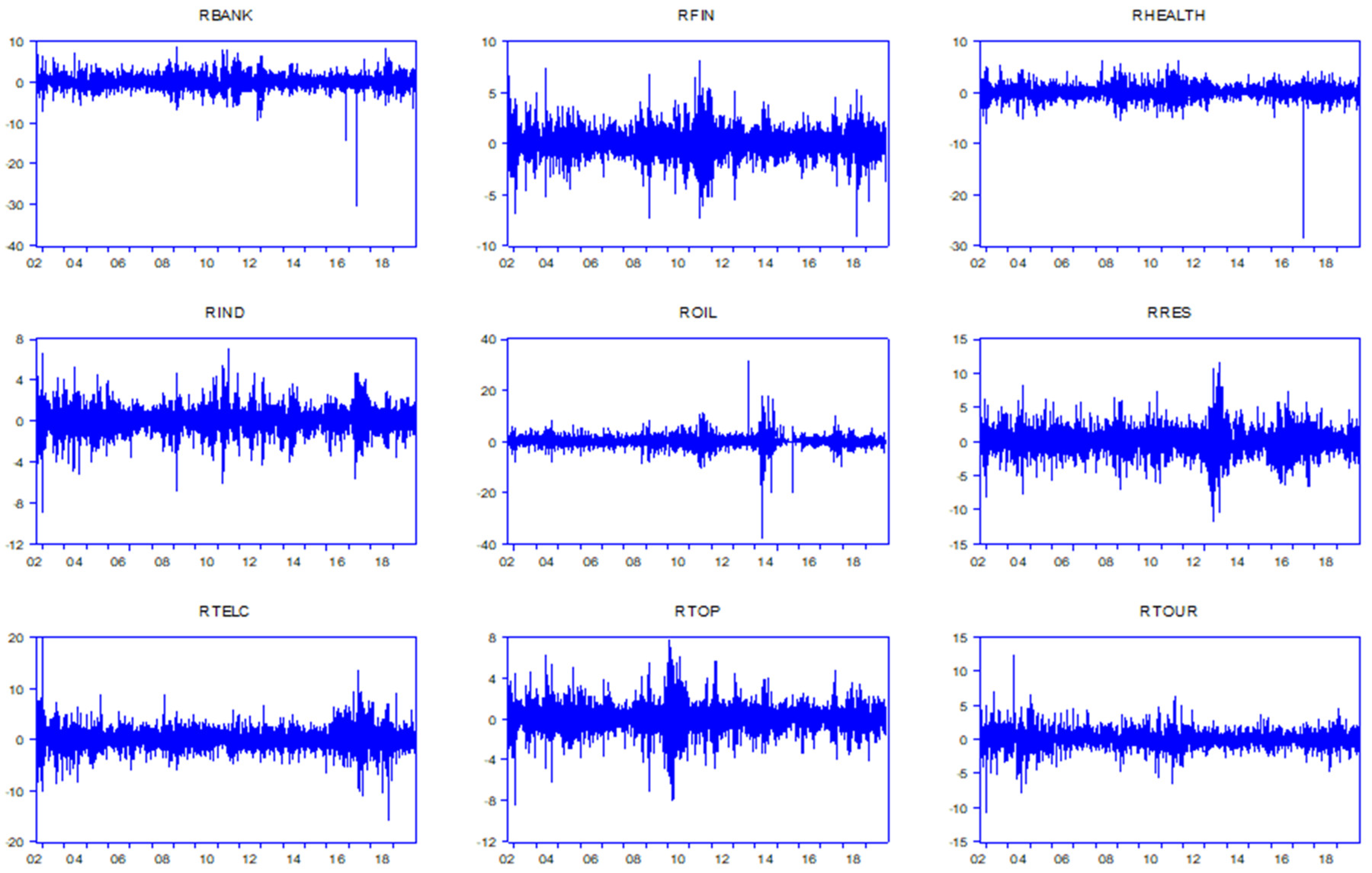
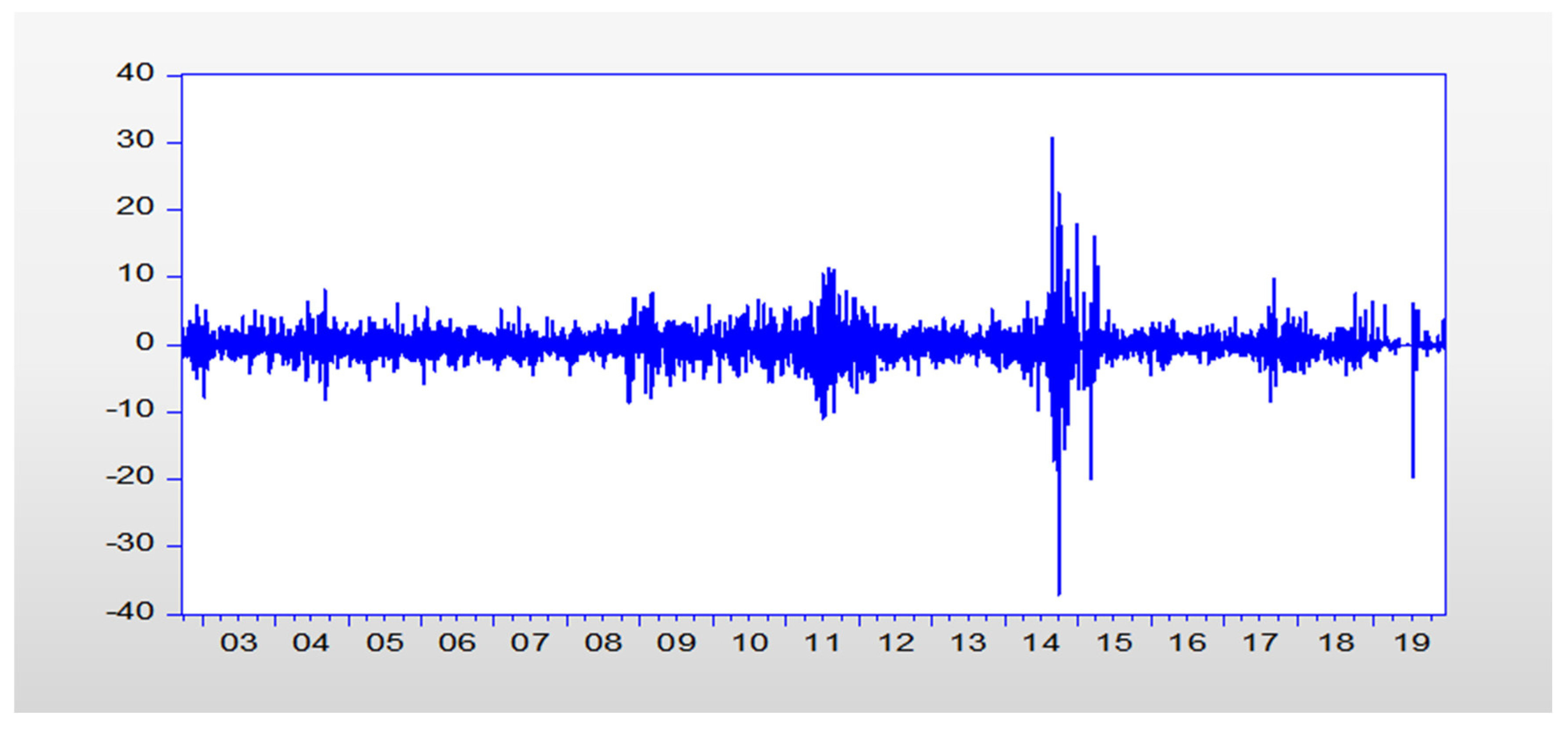
4.1. Data Description

This study uses 39,033 observations for the period 23 September 2002, to 20 December 2019. These are daily observations of the South African index compiled by the daily closing values of the Financial Time Stock Exchange/Johannesburg Stock Exchanges (FTSE/JSE) of bank index; financial index; healthcare index; industrial index; oil index; resources index; telecommunications index; top 40 index; and tourism index. The prices of all commodities are in US dollars. The dataset was gathered from Inet BFA, and the data availability defined the investigation timeframe.

The returns are calculated using Equation (1). Consequently, all indexes were transformed accordingly. Therefore, Rbank, Rfin, Rhealth, Rind, Rres, Rtel, Rtop, and Rtour stand, respectively, for bank returns, financial returns, healthcare returns, industrial returns, resources returns, telecommunications returns, top 40 returns, and tourism returns. A preliminary statistical analysis is performed, prior the estimation of suitable models. The software programs used are: Eviews 11, R 4.0.5; and MATLAB 9.1.

4.2. Descriptive Statistics and Preliminary Analysis

Table 1. Descriptive statistics of South African stock market log-returns.

	Rbank 1	Rfin 2	Rhealth 3	Rind 4	Roil 5	Rres 6	Rtelc 7	Rtop 8	Rtour 9
Mean	0.034	0.031	0.054	0.050	0.056	0.025	0.04	0.042	0.041
Std. Dev	1.731	1.356	1.328	1.207	2.342	1.861	2.051	1.331	1.206
Kurtosis	27.156	6.309	53.051	6.096	33.303	6.282	8.358	6.34	10.09
Skewness	−1.239	−0.054	−2.303	−0.182	−0.144	−0.007	0.121	−0.125	−0.029
Minimum	−30.214	−9.112	−28.459	−8.96	−37.586	−11.815	−15.915	−8.393	−10.674
Maximum	9.181	8.098	6.281	7.173	31.078	11.45	19.65	7.707	12.291
Jarque-Bera	9556.512	1980.179	456,527	1755.73	79,355.46	1946.217	5199.083	2098.731	9086.147
Size	4337	4337	4337	4337	4337	4337	4337	4337	4337

Source: Author’s calculation, E-views software was used to obtain the results, Std. Dev corresponds to standard deviation. 1 Rbank stands for bank returns; ² Rfin stands for financial returns; ³ Rhealth stands for healthcare returns; ⁴ Rind stands for industrial returns; ⁵ Roil stands for oil returns; ⁶ Rres stands for resource returns; ⁷ Rtelc stands for telecommunication returns; ⁸ Rtop stands for Top40 returns; ⁹ Rtour stands for tourism returns.

contains a few descriptive statistics about the returns. Oil returns have the highest standard deviation of all variables (2.342), implying that they are more volatile than other returns, followed by healthcare returns (2.051) and bank returns (1.731), while tourism returns have the lowest standard deviation (1.206), implying that they are less volatile. Healthcare returns have the highest kurtosis (53.051), followed by oil returns (33.303) and bank returns (27.156), indicating that all variables are leptokurtic. Most variables are found to have a negative skewness, except for the telecommunication returns (0.121), indicating that most series returns are spread on the left, indicating negative asymmetry and implying that the left tail of the dispersion is heavier. The Jarque–Bera test confirms that none of the variables are regularly distributed. As a result, the returns series exhibits a nonlinear phenomenon. All of these statistics are consistent with what has been reported in the financial literature.

Looking at the correlation coefficients in

Table 2. Linear correlation among all South African stock log-returns.

	Rbank	Rfin	Rhealth	Rind	Roil	Rres	Rtelc	Rtop	Rtour
Rbank	1
Rfin	0.806	1
Rhealth	0.385	0.527	1
Rind	0.435	0.552	0.442	1
Roil	0.179	0.295	0.227	0.249	1
Rres	0.190	0.274	0.230	0.319	0.350	1
Rtelc	0.316	0.355	0.234	0.402	0.102	0.148	1
Rtop	0.414	0.549	0.410	0.565	0.312	0.433	0.328	1
Rtour	0.243	0.336	0.256	0.231	0.140	0.126	0.145	0.207	1

Source: Author’s calculation, E-views software was used to obtain the results.

, the strongest positive linear relationship appears between financial and banking returns (0.806). The linear coefficient values for oil rates of return and other stock market returns range from 0.102 to 0.350, indicating a positive low linear correlation with other stock market returns. Because it presupposes that the pairings of data have linear qualities, assessing linear correlation might produce deceptive findings. As a result, the best evaluative tool should not be linear.

Figure 1 depicts time plots of South African sectoral stock market returns. All time plots depict the stylized phenomenon of volatility clustering, in which large (small) returns are followed by large (small) returns. The same plots show the impact of the financial crisis, which is described by large deviations in the return series. For example, oil returns decreased significantly between late 2014 and early 2016, owing to a drop in oil prices caused by a growing supply glut caused by leading oil producers such as Saudi Arabia’s refusal to cut output. As formerly specified, these issues will be addressed by a dynamic time-varying copula based on asymmetric GARCH models. In the end, the benefits of significantly lower oil prices were masked by the sluggish response of major oil-importing developing economies to economic activity (Stocker et al. 2018). The banking sector reveals a decrease from 2012 to 2013, as well as a poor performance in the second half of 2016 and the lowest point in 2017. This situation may be related to the political scandal engulfing the US-based management McKinsey and Company.

4.3. Empirical Results

It is essential to establish a fitting marginal distribution to the residuals, which is used to establish the multivariate model. Thus, the flow starts from oil volatility to the bivariate model.

4.3.1. Volatility Models (Marginal Distributions)

The coefficients ${\alpha }_1$ and ${\beta }_1$ from

Table 3. Oil volatility: AR (1) – GJR-GARCH (1, 1) estimated results.

	“Student Distribution”	“Skewed Student Distribution”
Mean Equation
$b_0$	0.0375 * (0.019)	0.0422 (0.018)
$b_1$	−0.0273 * (0.230)	−0.2751 * (0.228)
Variance Equation
w	0.0615 ** (−0.125)	0.0617 (0.153)
${\alpha }_1$	0.115 * (0.008)	0.115 * (0.0031)
${\beta }_1$	0.851 * (0.043)	0.8504 * (−0.534)
$\gamma$	0.0667 * (0.0119)	0.0657 * (0.001)
Shape	5.0036 * (0.273)	5.0046 * (0.237)
Skew		1.0114 * (0.020)
Log-likelihood	−8598.439	−8598.275
AIC	3.9692	3.9688
BIC	3.9825	3.9806

Notes: The language for statistical computing R was used to obtain the log-likelihood statistics, AIC, and BIC. With standard errors in parenthesis. *, ** represents significance at 1%, and 5%, respectively. Source: Author’s calculation.

are significant, confirming that the series has volatility segmentation effects. The GJR-GARCH approach does not violate the non-negativity constraints, as for each structure, ${\alpha }_1+\gamma =0.1816 and 0.1811, all\ge 0$. The model further considers the leverage effect, with all $\gamma =0.0667 and 0.0657, all\ge 0$. The AIC and BIC criteria imply that the model with the lowest value is the best model to fit the dataset for further enactments. Following Wang and Liu (2006), this study used AIC and BIC for comparing non-nested models. Given that the lowest AIC “3.9688” and BIC “3.9806” criterion values are attributed to the skewed student, therefore the skewed student models will fit oil price volatility more effectively than the student distribution if the GJR-GARCH structure is chosen.

Table 4. Oil volatility: AR (1)-E-GARCH (1, 1) estimated results.

	“Student Distribution”	“Skewed Student Distribution”
Mean Equation
$b_0$	0.0096 ** (0.004)	0.0097 * (0.004)
$b_1$	0.0270 * (0.012)	0.0272 * (0.012)
Variance Equation
w	0.0057 * (0.002)	0.0058 * (0.002)
${\alpha }_1$	0.0176 * (0.007)	0.0175 * (0.008)
${\beta }_1$	0.9930 * (0.000)	0.9930 * (0.000)
$\gamma$	−0..2327 * (0.012)	−0.2326 * (0.010)
Shape	4.4058 * (0.261)	4.4096 * (0.278)
Skew		1.0024 * (0.019)
Log-likelihood	−8540.415	−8540.423
AIC	3.9507	3.9512
BIC	3.9610	3.9630

Notes: R was used to obtain the log-likelihood statistics, AIC, and BIC. With standard errors in parenthesis. *, ** represents significance at 1%, and 5%, respectively. Source: Author’s calculation.

shows the results of the AR (1)-E-GARCH (1, 1) model. Because the conditional variance dynamic ${\mathrm{l}\mathrm{o}\mathrm{g}(\sigma }_t^2)$ is positive at any given period, the non-negativity constraint is respected; for all log-returns, the asymmetric terms “$\gamma =-0.2327 \mathrm{a}\mathrm{n}\mathrm{d}-0.2326$“ are negative; these results refer to a negative relationship between volatility and return for oil variable; and thus the EGARCH model accounts for the leverage effect. This means that a negative shock affects oil volatility more than a positive shock of comparable magnitude. Given that the coefficients ${\alpha }_1$ and ${\beta }_1$ are significant, the series exhibits volatility clustering effects. Negative shock persistence, also known as volatility asymmetry, suggests that investors are more susceptible to bad news than positive news. In other words, the volatility spillover mechanism is asymmetric, and the student distribution is the most suitable structure, rather than the skewed student distribution, based on the lowest values of the AIC “3.9510” and BIC “3.9610” criterion.

Figure 2 shows that oil volatility increased in 2008, between 2011 and 2012, and primarily in 2014 and 2015, implying the effect of the financial crisis, to end with volatility patterns, with high volatility tailed by high volatility and low volatility tailed by lower volatility.

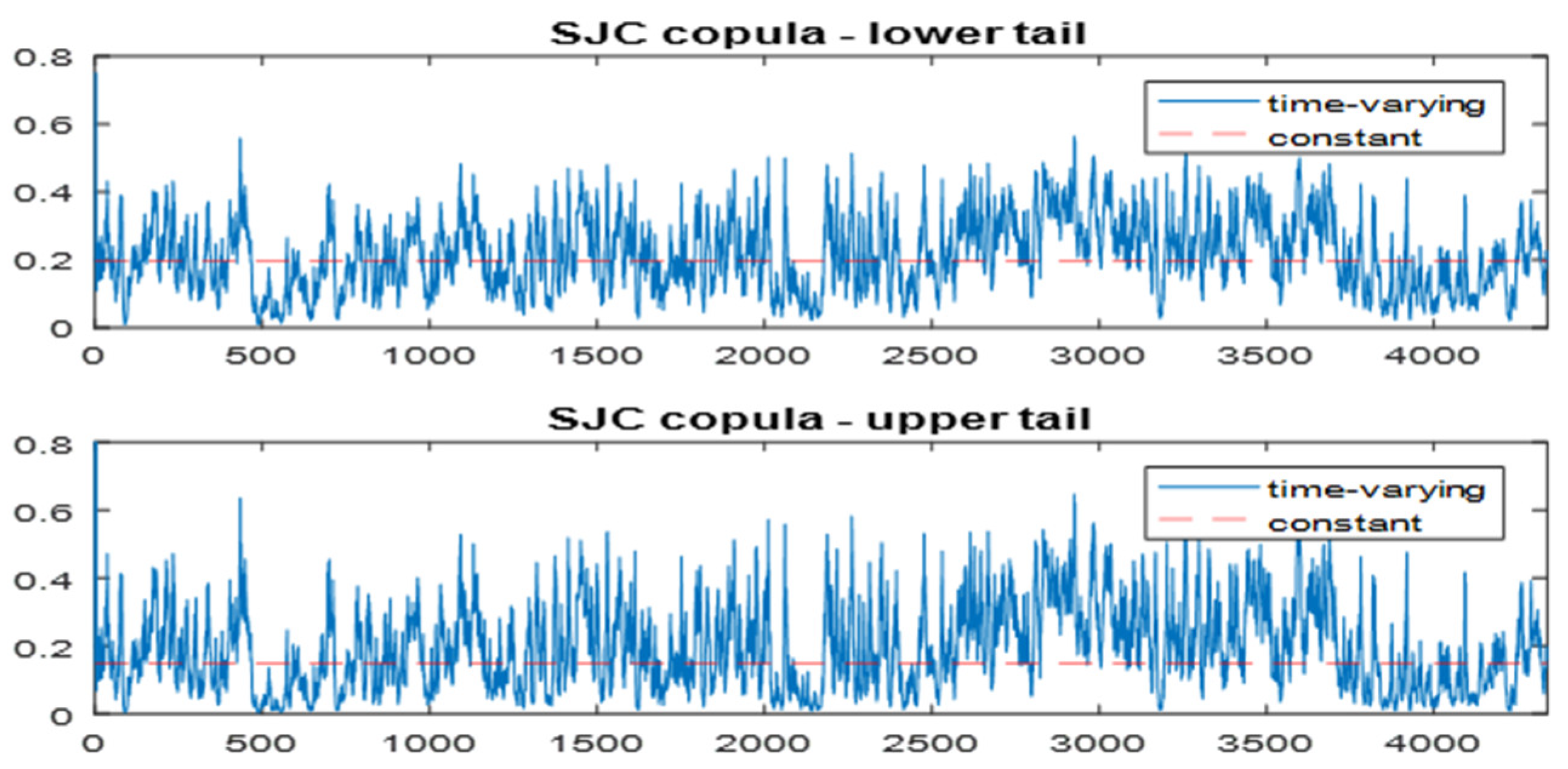
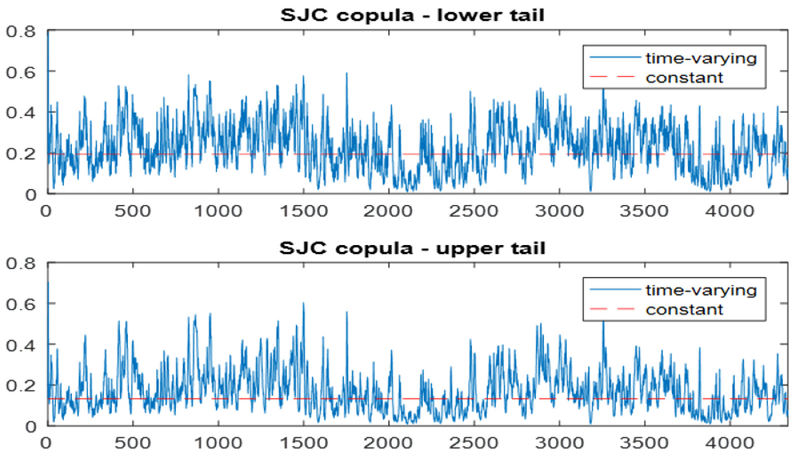
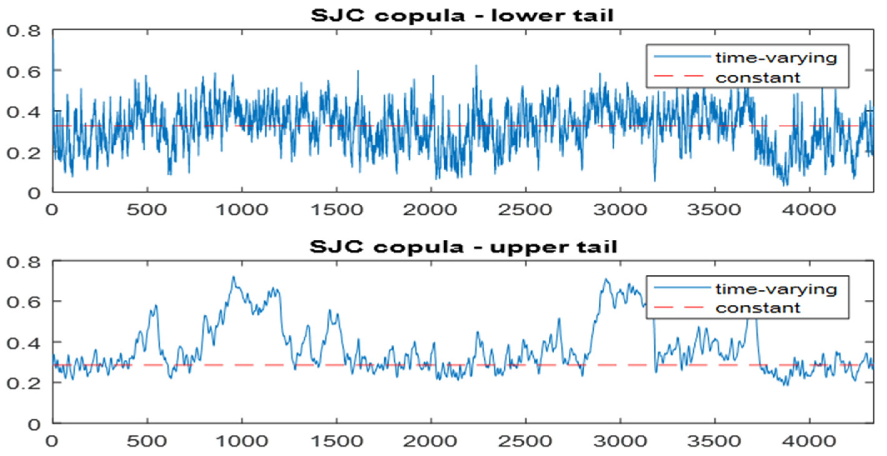
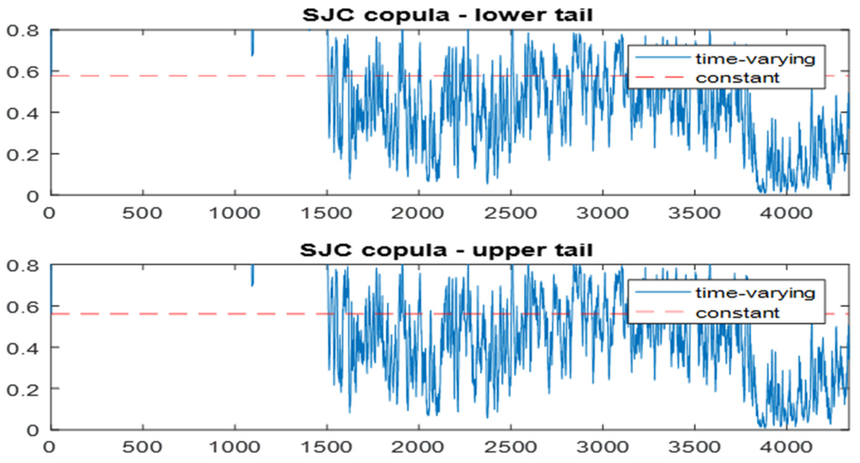
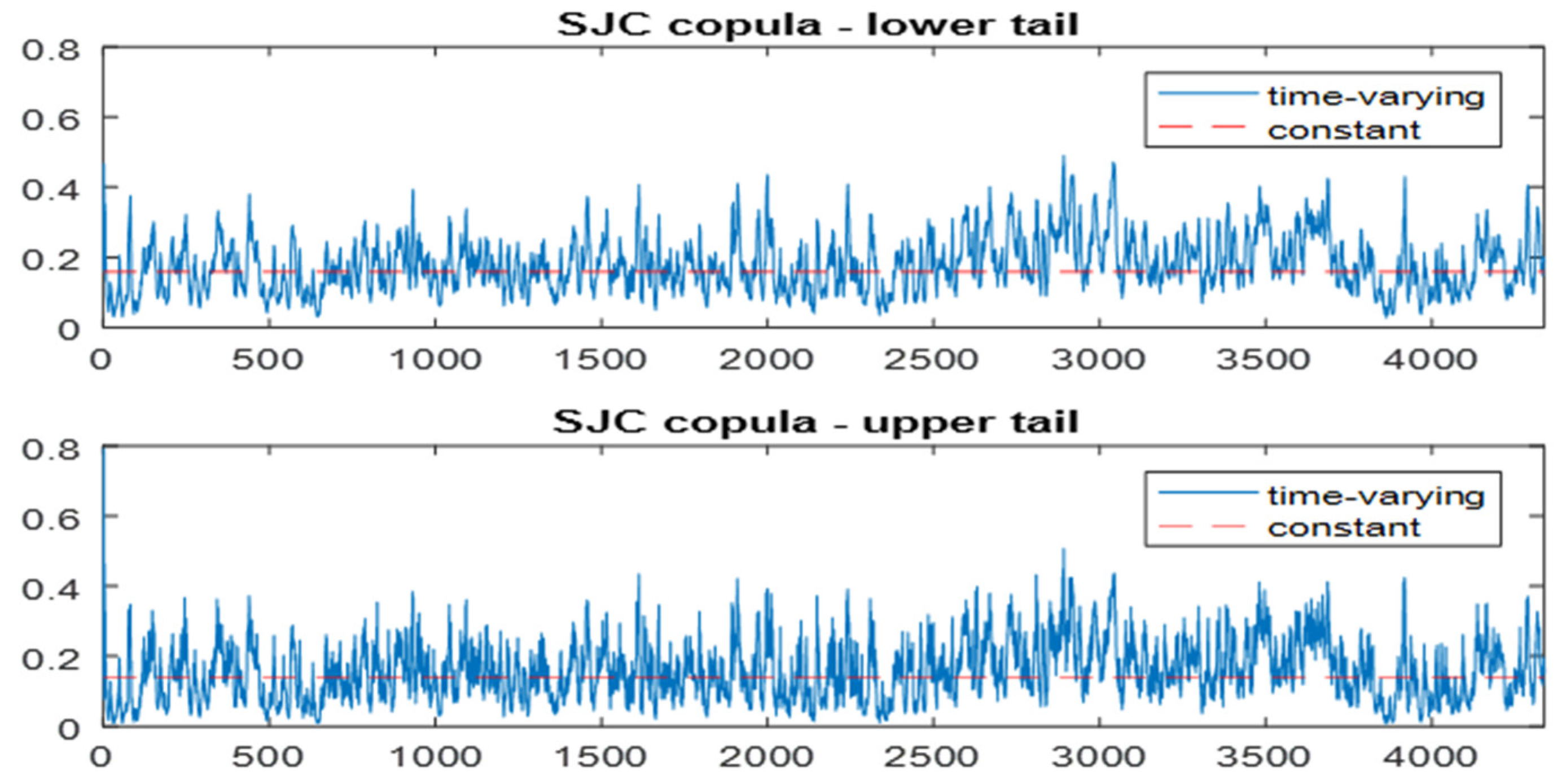
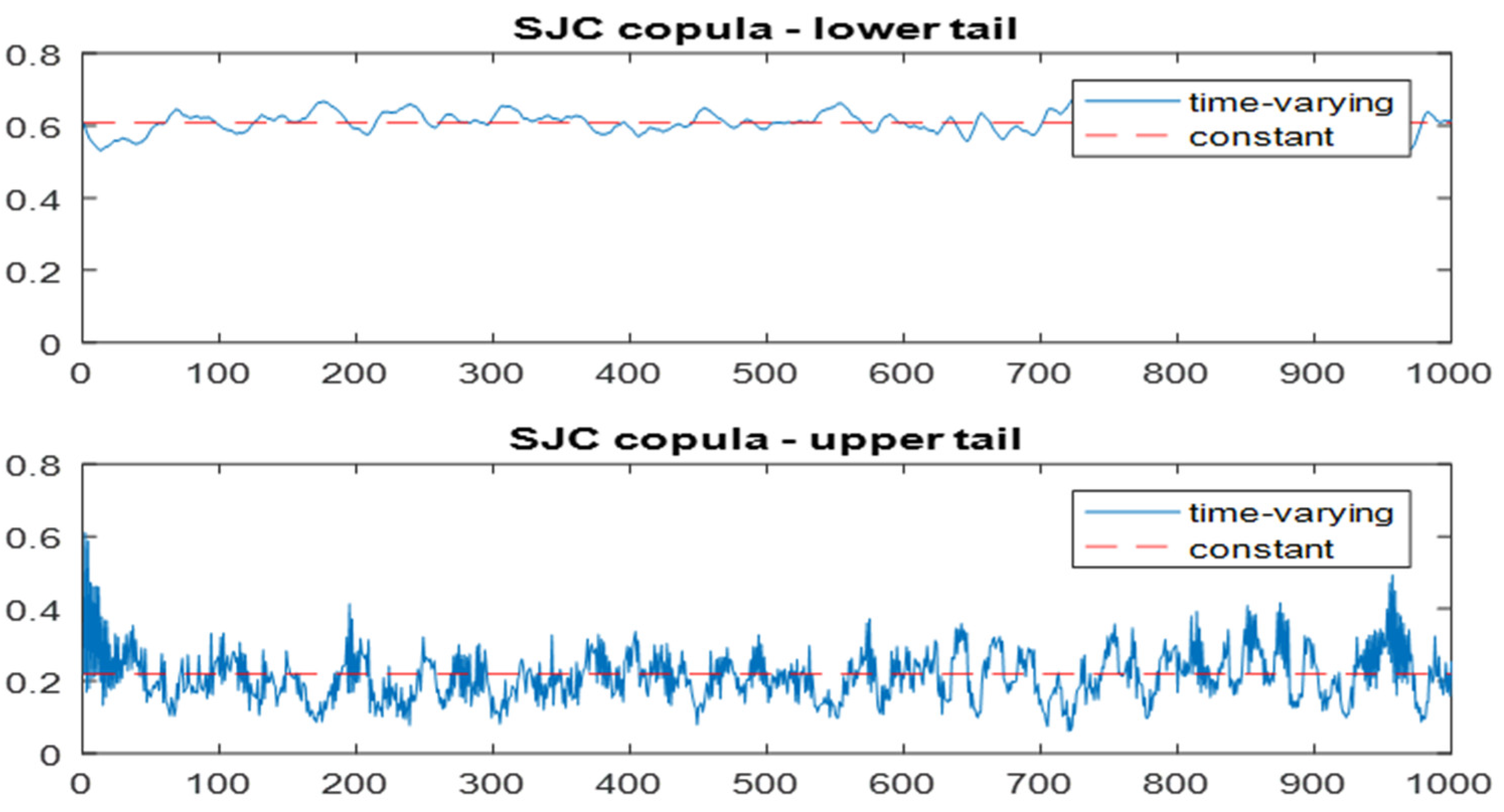
4.3.2. Bivariate Symmetrized Joe-Clayton (SJC) Copula

The SJC copulas can capture different types of interdependence, such as constant and time-varying relationships. Regarding tail disparity and dependence, for the upper and lower tails of each pair, the SJC copula is used to describe the occurrence of the dependent structure. Therefore, Equations (20)–(22) are used to evaluate the two-variable symmetric Joe-Clayton copula (SJC). Table 4 shows the constant and time-varying components of the SJC copula. In addition, it presents the returns of each South African stock market and the fluctuating oil prices, as well as the copula log-likelihood, AIC, BIC criterion, and standard errors for the SJC time-varying copula models (Patton 2012).

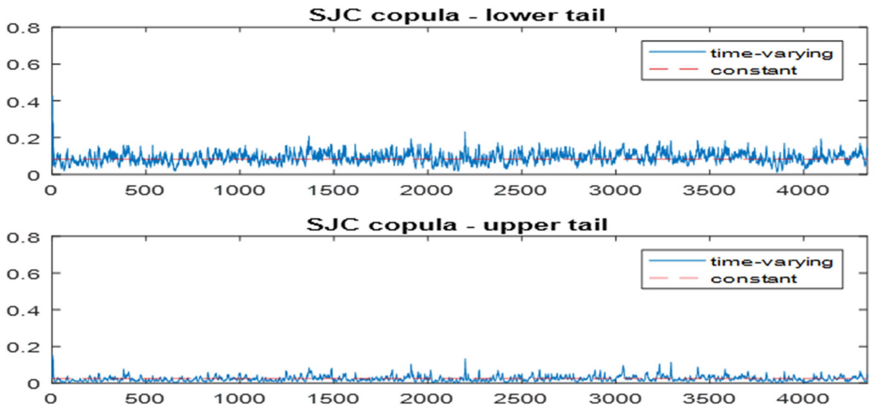
4.3.3. Symmetrized Joe-Clayton (SJC) Copula

Based on the results of

Table 5. Estimated SJC of oil price volatility and stock market returns.

	Oil-Banks	Oil-Financials	Oil-Healthcare	Oil-Industrials	Oil-Resources	Oil-Telecom	Oil-Top40	Oil-Tourism
Constant symmetrized Joe Clayton (SJC)
${\tau }^U$	0.157 * (0.022)	0.223 * (0.023)	0.132 * (0.023)	0.327 * (0.020)	0.575 * (0.018)	0.159 * (0.022)	0.234 * (0.017)	0.023 (0.014)
${\tau }^L$	0.195 * (0.021)	0.270 * (0.021)	0.192 * (0.021)	0.376 * (0.022)	0.561 * (0.019)	0.195 * (0.021)	0.612 * (0.017)	0.080 * (0.018)
AIC	−590.43	−919.55	−548.15	−1259.54	−3409.90	−495.12	−3000.43	−182.79
BIC	−577.68	−906.80	−535.41	−1246.79	−3397.15	−482.38	−2987.68	−170.04
Likelihood	297.26	461.77	276.14	631.77	1706.96	249.56	1502.21	93.39
Time-varying symmetrized Joe Clayton (SJC)
${\omega }^U$	0.156 (0.075) *	0.159 (0.054) *	0.114 (0.028) *	0.238 (0.046) *	0.171 (0.014) *	0.127 (0.041) *	0.174 (0.034) *	1.521 (0.508) *
${\alpha }^U$	−1.120 (0.227) *	−0.678 (0.226) *	−0.794 (0.286) *	−0.474 (0.228) *	−0.678 (0.321)	−0.813 (0.168) *	−0.476 (0.090) *	−1.864 (0.803) *
${\beta }^U$	0.963 (0.008) *	0.971 (0.240) *	0.965 (0.015) *	0.976 (0.011) *	0.980 (0.019) *	0.969 (0.010) *	0.975 (0.003) *	0.876 (0.064) *
${\omega }^L$	0.149 (0.049) *	0.954 (0.487)	0.105 (0.063)	1.362 (0.401) *	0.723 (0.475)	0.095 (0.017) *	0.140 (0.027) *	1.527 (0.963)
${\alpha }^L$	−9.964 (1.675) *	−0.823 (0.443)	−9.258 (3.135) *	−0.604 (0.299)	−0.848 (0.561) *	−6.958 (2.949)	−0.748 (0.363) *	−8.960 (3.522) *
${\beta }^L$	0.042 (0.016) *	0.938 (0.211) *	0.177 (0.259)	0.970 (0.024) *	0.975 (0.019) *	0.172 (0.305)	0.986 (0.016) *	0.732 (0.246) *
AIC	−806.30	−1179.38	−686.56	−1512.42	−5316.18	−574.85	−4024.60	−191.30
BIC	−768.05	−1141.13	−648.33	−1474.17	−5277.93	−536.61	−3983.35	−153.04
Likelihood	409.15	461.69	349.28	762.21	2664.09	293.42	2016.80	101.65

Notes: MATLAB was used to attain the parameters (Dynamic Toolbox), “*”significant level = 0.05. With standard errors in parenthesis. Sources: Author’s calculations.

, the constant measures of dependency (τ^L, τ^U) present a reasonable estimate of the correlation for the complete lower and upper tail dependency, given statistically significant parameters for most pairs. Nonetheless, the constant component of SJC appears unsuitable for unfolding the dependence behavior relating to stock market returns and oil price fluctuations, as its AIC and BIC criteria have higher values than the time-varying component. As a result, the time-varying method will be prioritized. As shown in Table 5, for the dynamic dependency of all pairs, all upper parameters ${\omega }^U$ are statistically significant, as are the majority of the lower ${\omega }^L$ except for the pairs oil–healthcare and oil–resources.

First, the upper dependence (${\omega }^U$) can be sorted in descending order r such that: oil–tourism > oil–industrials > oil–top 40 > oil–resources > oil–financials > oil–banks > oil–telecommunication > oil–healthcare. Second, the lower tail dependence (${\omega }^L$) between oil price volatility and other stock market returns is ranked in descending order as follows: oil–tourism > oil–industrials > oil–financials > oil–banks > oil–top 40 > oil–telecommunication.

As established, a heavy tail distribution equates to the parameter of dependence with the highest absolute value. As a result of the ranking, the dynamic fluctuations between oil price volatility and tourism returns over time have the strongest overall dependency, followed by the relationship between oil price volatility and industrial returns, oil price volatility and top 40, oil price volatility and resources, oil price volatility and financials, and oil price volatility and banks. Oil and healthcare returns in the upper tail have the weakest overall dependency, while oil price volatility and telecommunication returns in the lower tail have the weakest overall dependency. These findings are in line with the outcomes of Hamdi et al. (2019); they established that oil price volatility has no effect on telecommunication.

Thus, among several other stock market returns, oil price volatility has the greatest impact on tourism returns in losses (lower tail) or in high risk-taking decisions, assuming high returns (upper tail). The results likewise illustrate that most of the persistent coefficients $({\beta }^U,{\beta }^L)$ for all pairs are greater than the variation “adjustment” coefficient $({\alpha }^U,{\alpha }^L)$. These findings provide some insight in the evolution of interdependent structures for higher and lower extremities over time. In terms of persistence, as indicated by the parameter $\beta ({\beta }^U,{\beta }^L)$, more pairs are tenacious in the upper than in the lower tails, except for the pair oil–top 40, which is persistent in the lower tail (${\beta }^L=0.986>{\beta }^U=0.975)$. In fact, the most persistent dependencies are oil–resources (${\beta }^U=0.980)$, oil–healthcare (${\beta }^U=0.976)$, and oil–financials (${\beta }^U=0.971)$, whereas the pair oil–tourism (${\beta }^U=0.876)$ is the least persistent. For all pairs, the lower tail adjusts faster than the upper tail, because the absolute values of the lower tail are greater than the absolute values of the upper tail $(=\left|{\alpha }^L\right|>\left|{\alpha }^U\right|)$. The pair oil–banks ($\left|{\alpha }^L\right|=9.964$, followed by oil–industrials $\left|{\alpha }^L\right|=9.258$, and oil–tourism $\left|{\alpha }^L\right|=8.960$ are the quickest to correct, while the pair oil–healthcare ($\left|{\alpha }^L\right|=0.604)$ is the lowest.

To investigate the dynamic symbiotic relationship structure between fluctuating oil prices and stock returns further, based on the SJC time-varying model, we display the timelines for all lower, and upper extremity interconnections in Figure 3, Figure 4, Figure 5, Figure 6, Figure 7, Figure 8, Figure 9 and Figure 10 below. The results demonstrate that the measurement grounded on the constant component is insufficient to label the dependencies between the variables. Nonetheless, the constant indicator of reliance provided a reasonable estimate of the means of the plots’ fluctuations for overall dependency. The view of different figures provides different perspectives on the fluctuations of the upper and lower extremities dependency structures over time. We can obtain a sense of the time-varying tail reliance from these figures.

In Figure 3, the dependency patterns between oil volatility and bank returns are similar in the upper and lower tails, but the upper tail is more dependent than the lower tail; ${\omega }^U=0.156>{\omega }^L=0.149$, implying that, in the above, an increase in bank yields can be related either to an increase or decrease in oil prices.

Given that banks are risk-averse, the rational way to ensure increased bank returns must be linked to a reduction in oil prices’ fluctuation. Along the way, the co-movement adjusts faster in the upper tail, ${\alpha }^L=\left|-9.964\right|>{\alpha }^U=\left|-1.120\right|$. The higher extremity dynamic dependency is tougher compared to the lower extremity, ${\beta }^U=0.963>{\beta }^L=0.042$. Figure 4 depicts the SJC’s constant component’s failure to capture the dynamic dependency. The time-varying dependency curve evolved on either side of constant dependence. The results show that the parameters ${\omega }^L \mathrm{a}\mathrm{n}\mathrm{d} {\alpha }^L$ are not statistically significant; thus, only the co-movement in the upper tail is considered. Because of the strong dependence in the upper tail, a decrease in financial sectoral returns is expected if oil price volatility rises. From Figure 5, the path of time-varying dependency is higher than the path of constant dependency. The persistence parameter ${\beta }^L$ is not statistically significant, but the variation parameters show a quick adjustment of the lower tail compared to the upper tail, ${\alpha }^L=\left|-9.258\right|>{\alpha }^U=\left|-0.794\right|$, and the lesser tail dependency is effective compared to the higher tail dependency, ${\omega }^L=1.527>{\omega }^U=0.159$. This implies that a hike in oil price volatility may end in a loss in sectoral healthcare returns. In Figure 6, the shapes of dependency of oil volatility–industrial returns exhibit a higher volatility for the lesser extremity than for the higher extremity; additionally, the time-varying path in the higher extremity moves above the constant dependence, whereas for the lower tail, the curve of the time-varying dependency evolves on either side of the constant dependency. Because the parameters ${\omega }^L$ and ${\alpha }^L$ are statistically insignificant, the emphasis is on the upper tail dependency. The dependency paths in Figure 7 exhibit a much higher volatility in the lower and upper tails. The dynamic dependency correlation is more reliable in the higher extremity as opposed to the lesser extremity,${\beta }^U=0.980>{\beta }^L=0.975$; simultaneously, the lower tail dependency regulates faster than the upper tail, ${\alpha }^L=\left|-0.848\right|>{\alpha }^U=\left|-0.678\right|$, and the dependency is stronger in the higher extremity than in the lesser extremity, ${\omega }^U=0.171>{\omega }^L=0.140$. Oil price volatility is likely to cause an increase in sectoral resource returns.

The dependence of oil volatility and telecommunications returns follows a similar pattern in the upper and lower tails, as shown on Figure 8. Because the lower tail dependency parameter ${\omega }^L$ is statistically insignificant, the upper tail dependency adequately explains the connection between fluctuating oil prices and telecommunication returns. However, as explained above, the impact of oil prices on telecommunication returns is slender even in the upper tail dependency. Considering Figure 9, the dependency is rather stable in the lower extremity and moderately volatile in the upper extremity. There is more dynamic dependency persistence in the lesser extremity as opposed to the higher tail,${\beta }^L=0.986>{\beta }^U=0.975$, and the adjustment process is faster in the lower tail than in the upper tail, ${\alpha }^L=\left|-0.748\right|>{\alpha }^U=\left|-0.476\right|$, and the dependency in the higher extremity is stronger than the reliance in the lesser extremity, ${\omega }^U=0.156>{\omega }^L=0.095$. Lessening oil price volatility will result in a surge for the top 40 returns. Based on Figure 10, the dependency in the upper tail is more consistent and stronger than in the lesser tail as opposed to in the higher tail, ${\omega }^L=1.527>{\omega }^U=1.521$, suggesting that any oil prices’ fluctuation hike is likely to negatively affect the tourism returns. The co-movement corrects faster in the lesser extremity as opposed to the higher extremity, ${\alpha }^L=\left|-8.960\right|>{\alpha }^U=\left|-1.864\right|$. Losses in tourism returns appear to be a result of increased oil price volatility. The dynamic dependency is more stable in the higher extremity dependency than in the lesser extremity dependency,${\beta }^U=0.876>{\beta }^L=0.732$. Given that tourism is more reliant on transportation, the outcomes of the study contrast with the findings of Hamdi et al. (2019), that show a surprising independence of transport returns to oil prices’ volatility.

5. Conclusions

This study looked at the moving in tandem of oil price fluctuations and South African stock market returns. The study used 39,033 observations of the South African index compiled by daily closing values of the Financial Time Stock Exchange/Johannesburg Stock Exchanges (FTSE/JSE) of the bank index; financials index; healthcare index; industrials index; oil index; resources index; telecommunications index; top 40 index; and tourism index, for the period 23 September 2002 to 20 December 2019. The results of the bivariate SJC copula’s dependence structure, based on the E-GARCH oil volatility model, indicate an asymmetric impact of oil price fluctuations on stock market returns, via time-varying dependence parameters in extreme situations, which imply the existence of co-movement between oil price volatility and South African stock returns. The existence of left/right tail reliance indicates a substantially higher risk of going down/up in returns when fluctuating oil prices are present. The findings reveal that the tourism industry is the most vulnerable to fluctuations in oil prices. Other sectors that are dependent on oil price volatility include industrials, the top 40, telecommunications, healthcare, and resource returns. As such, oil price volatility may be the cause of lower output. These findings differ significantly from previous findings in the literature. Previous research has discovered that oil volatility and the industrial sector index have a negative association, and it has been demonstrated that oil price shocks have a negative impact on transportation, financial services, and manufacturing (Arouri 2011; Phan et al. 2015).

On the policy font, the study suggests that policymakers must place a high priority on areas that are susceptible to change in oil prices. In the short run, an expansionary monetary policy can be used to soften the impact of increasing oil prices; as inflation rate hikes due to increased money in circulation are controlled. In the meantime, because of economic growth activities that lead to the increase in stock market returns, the impact of oil prices increase can be tempered by the outcomes of the improved stock market returns. However, in the long term, the government can develop a policy framework to prevent this effect. The study’s main policy implication is that reducing oil volatility (by lowering oil prices) will help to reduce the negative effect that oil volatility has on stock returns. The major challenge is that, while price stability is important for overall macroeconomic management, oil prices are determined by demand, supply, and speculative factors all over the world. Lower prices lower production costs, which benefit customers by assuring reasonable product prices and, as a result, greater demand and expenditure. Rising shares and gains, which are the primary stock markets drivers, benefit producers as well. The asymmetric effect in the findings, on the other hand, suggests that lower costs may not always translate into higher output. Overall, actions that limit price fluctuations will enhance the South African stock market. This is because such policies will benefit South African economic growth via the exchange rate channel, by lowering import bills and increasing exports. As a result, the importance of maintaining stable oil prices cannot be overstated.

On the other hand, it is worth noting that the South African energy market exhibits notable market failures, notably negative externalities, which in turn hampers the optimization of economic efficiency and welfare. The externalities associated within the South African oil market include inter-alia climate change, environmental damage emanating from oil extraction and refining, and air and water pollution. The study therefore recommends that policymakers seek to make the market more efficient by removing barriers in both forward and future oil markets. This could possibly happen if policy makers implement regulations, including strict environmental standards, emission controls, and externality pricing. Analyzing the results derived from this study reveals that exploring VaR (value at risk) and ES (expected shortfall) is a crucial avenue to consider for future research (See He and Hamori 2019).

References

1. Alzyoud, H., E. Z. Wang, and M. G. Basso. 2018. Dynamics of Canadian oil price and its impact on exchange rate and stock market. International Journal of Energy Economics and Policy 8: 107–14. [Google Scholar]
2. Arouri, E. M., and K. D. Nguyen. 2010. Oil prices, stock markets and portfolio investment:Evidence from sector analysis in Europe over the last decade. Energy Policy 38: 4528–39. [Google Scholar] [CrossRef]
3. Arouri, M. E. H. 2011. Does crude oil move stock markets in Europe? A sector investigation. Economic Modelling 28: 1716–25. [Google Scholar] [CrossRef]
4. Başkaya, Y. S., T. Hülagü, and H. Küçük. 2013. Oil price uncertainty in a small open economy. IMF Economic Review 61: 168–98. [Google Scholar] [CrossRef]
5. Beckmann, J., T. Berger, and R. Czudaj. 2016. Oil price and FX-rates dependency. Quantitative Finance 16: 477–88. [Google Scholar] [CrossRef]
6. Bollerslev, T. 1986. Generalized autoregressive conditional heteroskedasticity. Journal of Econometrics 31: 307–27. [Google Scholar] [CrossRef]
7. Bouri, E. 2015. Oil volatility shocks and the stock markets of oil-importing MENA economies: A tale from the financial crisis. Energy Economics 51: 590–98. [Google Scholar] [CrossRef]
8. Cai, X., S. Hamori, L. Yang, and S. Tian. 2020. Multi-Horizon Dependence between Crude Oil and East Asian Stock Markets and Implications in Risk Managementk. Energies 13: 294. [Google Scholar] [CrossRef]
9. Choi, K., and S. Hammoudeh. 2010. Volatility behavior of oil, industrial commodity and stock markets in a regime-switching environment. Energy Policy 38: 4388–99. [Google Scholar] [CrossRef]
10. Dai, Z., and H. Zhu. 2022. Time-varying spillover effects and investment strategies between WTI crude oil, natural gas and Chinese stock markets related to belt and road initiative. Energy Economics 108: 105883. [Google Scholar] [CrossRef]
11. Diebold, F. X., and K. Yilmaz. 2012. Better to give than to receive: Predictive directional measurement of volatility spillovers. International Journal of forecasting 28: 57–66. [Google Scholar] [CrossRef]
12. Diebold, F. X., and K. Yılmaz. 2014. On the network topology of variance decompositions: Measuring the connectedness of financial firms. Journal of Econometrics 182: 119–34. [Google Scholar] [CrossRef]
13. Dutta, A., J. Nikkinen, and T. Rothovius. 2017. Impact of oil price uncertainty on Middle East and African stock markets. Energy 123: 189–97. [Google Scholar] [CrossRef]
14. Elyasiani, E., I. Mansur, and B. Odusami. 2013. Sectoral stock return sensitivity to oil price changes: A double-threshold FIGARCH model. Quantitative Finance 13: 593–612. [Google Scholar] [CrossRef]
15. Engle, R. F. 1982. Autoregressive conditional heteroscedasticity with estimates of the variance of united kingdom inflation. Econometrica 58: 987–1007. [Google Scholar] [CrossRef]
16. Engle, R. F. 1990. Stock volatility and the crash of’87: Discussion. The Review of Financial Studies 3: 103–6. [Google Scholar] [CrossRef]
17. Engle, R. F., and V. K. Ng. 1993. Measuring and testing the impact of news on volatility. The Journal of Finance 48: 1749–78. [Google Scholar] [CrossRef]
18. Eyden, R. V., M. Difeto, R. Gupta, and M. E. Mark. 2019. Oil price volatility and economic growth: Evidence from advanced economies using more than a century’s data. Applied Energy 233: 612–21. [Google Scholar] [CrossRef]
19. Feng, J., Y. Wang, and L. Yin. 2017. Oil volatility risk and stock market volatility predictability: Evidence from G7 countries. Energy Economics 18: 240–54. [Google Scholar] [CrossRef]
20. Ferdi, K., and E. Yildirim. 2014. The causal effect of shifting oil to natural gas consumption oncurrent account balance and economic growth in 11 OECDcountries: Evidence from bootstrap-corrected panel causality test. Social and Behavioral Sciences 143: 1064–69. [Google Scholar]
21. Filis, G., S. Degiannakis, and C. Floros. 2011. Dynamic correlation between stock market and oil prices: The case of oil-importing and oil-exporting countries. International Review of Financial Analysis 20: 152–64. [Google Scholar] [CrossRef]
22. Glosten, L., R. Jagannathan, and D. Runkle. 1993. On the relation between expected value and the volatility of the nominal excess return on stocks. Journal of Finance 48: 1779–801. [Google Scholar] [CrossRef]
23. Gupta, R., and M. P. Modise. 2013. Does the source of oil price shocks matter for South African stock returns? A structural VAR approach. Energy Economics 40: 825–31. [Google Scholar] [CrossRef]
24. Hamdi, B., M. Aloui, F. Alqahtani, and A. Tiwari. 2019. Relationship between the oil price volatility and sectoral stock markets in oil-exporting economies: Evidence from wavelet nonlinear denoised based quantile and Granger-causality analysis. Energy Economics 80: 536–52. [Google Scholar] [CrossRef]
25. Hamma, W., A. Jarboui, and A. Ghorbel. 2014. Effect of oil price volatility on Tunisian stock market at sector-level and effectiveness of hedging strategy. Procedia Economics and Finance 13: 109–27. [Google Scholar] [CrossRef]
26. He, Y., and S. Hamori. 2019. Conditional dependence between oil prices and exchange rates in BRICS countries: An application of the copula-GARCH model. Journal of Risk and Financial Management 12: 99. [Google Scholar] [CrossRef]
27. He, Y., T. Nakajima, and S. Hamori. 2020. Can BRICS’s currency be a hedge or a safe haven for energy portfolio? An evidence from vine copula approach. The Singapore Economic Review 65: 805–36. [Google Scholar] [CrossRef]
28. Jones, C. M., and G. Kaul. 1996. Oil and the stock markets. Journal of Finance 51: 463–91. [Google Scholar] [CrossRef]
29. Joo, Y. C., and S. Y. Park. 2021. The impact of oil price volatility on stock markets: Evidences from oil-importing countries. Energy Economics 101: 105413. [Google Scholar] [CrossRef]
30. Li, J., and P. Li. 2021. Empirical analysis of the dynamic dependence between WTI oil and Chinese energy stocks. Energy Economics 93: 104299. [Google Scholar] [CrossRef]
31. Naeem, M., Z. Umar, S. Ahmed, and E. M. Ferrouhi. 2020. Dynamic dependence between ETFs and crude oil prices by using EGARCH-Copula approach. Physica A: Statistical Mechanics and Its Applications 557: 124885. [Google Scholar] [CrossRef]
32. Nelson, D. B. 1991. Conditional heteroskedasticity in asset returns: A new approach. Econometrica 59: 347–70. [Google Scholar] [CrossRef]
33. OPEC. 2020. Press Release for the OPEC 179th Meeting of the Conference Concludes. Available online: https://www.opec.org/opec_web/en/press_room/5963.htm#:~:text=The%20179th%20Meeting%20of,welcomed%20new%20ministers%3A%20HE%20Dr (accessed on 3 June 2023).
34. Patton, A. J. 2006. A Review of Copula Models for Economic Time Series. Journal of Multivariate Analysis 110: 4–18. [Google Scholar] [CrossRef]
35. Patton, A. J. 2012. Modelling asymmetric exchange rate dependence. International Economic Review 47: 527–56. [Google Scholar] [CrossRef]
36. Phan, D. H. B., S. S. Sharma, and P. K. Narayan. 2015. Oil price and stock returns of consumers and producers of crude oil. Journal of International Financial Markets, Institutions and Money 34: 245–62. [Google Scholar] [CrossRef]
37. Pirlogea, C., and C. Cicea. 2012. Econometric perspective of the energy consumption and economic growth relation in European Union. Renewable and Sustainable Energy Reviews 16: 5718–26. [Google Scholar] [CrossRef]
38. Silvapulle, P., R. Smyth, X. Zhang, and J. Fenech. 2017. Nonparametric panel data model for crude oil and stock prices in net oil importing countries. Energy Economics 67: 255–67. [Google Scholar] [CrossRef]
39. Sklar, M. 1959. Fonctions de répartition à n dimensions et leurs marges. Annales de l’ISUP 8: 229–31. [Google Scholar]
40. Stocker, M., J. Baffes, and D. Vorisek. 2018. What Triggered the Oil Price Plunge of 2014–2016 and Why It Failed to Deliver an Economic Impetus in Eight Charts. Washington, DC: World Babk GroupGlobal Economic Prospects. [Google Scholar]
41. Swanepoel, J. A. 2006. The impact of external shocks on South African inflation at different price stages. Journal for Studies in Economics and Econometrics 30: 1–22. [Google Scholar] [CrossRef]
42. Taylor, S. 1986. Modelling Financial Time Series. Chichester: Wiley. [Google Scholar]
43. Tiwari, A. K., I. D. Raheem, S. Bozoklu, and S. Hammoudeh. 2022. The oil price, macroeconomic fundamentals nexus for emerging market economies: Evidence from a wavelet analysis. International Journal of Finance and Economics 27: 1569–90. [Google Scholar] [CrossRef]
44. SA. Department of Energy. 2019. The South African Energy Sector Report. Available online: https://www.energy.gov.za/files/media/explained/2019-South-African-Energy-Sector-Report.pdf (accessed on 3 June 2023).
45. Valdés, A. L., L. A. Fraire, and R. D. Vázquez. 2016. A copula-TGARCH approach of conditional dependence between oil price and stock market index: The case of Mexico. Centro de Estudios Económicos 31: 47–63. [Google Scholar]
46. Wang, Y., and Q. Liu. 2006. Comparison of Akaike information criterion (AIC) and Bayesian information criterion (BIC) in selection of stock–recruitment relationships. Fisheries Research 77: 220–25. [Google Scholar] [CrossRef]
47. Wang, Y., C. Wu, and L. Yang. 2013. Oil price shocks and stock market activities: Evidence from oil-importing and oil-exporting countries. Journal of Comparative Economics 41: 1220–39. [Google Scholar] [CrossRef]
48. Yuan, X., J. Tang, W. K. Wong, and S. Sriboonchitta. 2020. Modeling Co-Movement among Different Agricultural Commodity Markets: A Copula-GARCH Approach. Sustainability 12: 393. [Google Scholar] [CrossRef]
49. Zhang, K. S., and Y. Y. Zhao. 2021. Modeling dynamic dependence between crude oil and natural gas return rates: A time-varying geometric copula approach. Journal of Computational and Applied Mathematics 386: 113243. [Google Scholar] [CrossRef]
Figure 1. Log-differenced series of the South African stock market index.
Economies 12 00004 g001
Figure 2. Plot for AR (1)-E-GARCH (1, 1) oil volatility.
Economies 12 00004 g002
Figure 3. Dependence path of the time-varying SJC: pair oil–banks.
Economies 12 00004 g003
Figure 4. Dependence path of the time-varying SJC: pair oil–financials.
Economies 12 00004 g004
Figure 5. Dependence path of the time-varying SJC: pair oil–healthcare.
Economies 12 00004 g005
Figure 6. Dependence path of the time-varying SJC: pair oil–industrial.
Economies 12 00004 g006
Figure 7. Dependence path of the time-varying SJC: pair oil–resources.
Economies 12 00004 g007
Figure 8. Dependence path of the time-varying SJC: pair oil–telecommunication.
Economies 12 00004 g008
Figure 9. Dependence path of the time-varying SJC: pair oil–top 40.
Economies 12 00004 g009
Figure 10. Dependence path of the time-varying SJC: pair oil–tourism.
Economies 12 00004 g010