A Comparative Analysis of the Choice of Mother Wavelet Functions Affecting the Accuracy of Forecasts of Daily Balances in the Treasury Single Account

Abstract

Improving the accuracy of cash flow forecasting in the TSA is key to fulfilling government payment obligations, minimizing the cost of maintaining the cash reserve, providing the absence of outstanding debt accumulation and ensuring investment in financial instruments to obtain additional income. This study aims to improve the accuracy of traditional methods of forecasting the time series compiled from the daily remaining balances in the TSAbased on prior decomposition using a discrete wavelet transform. The paper compares the influence of selecting a mother wavelet out of 570 mother wavelet functions belonging to 10 wavelet families (Haar;Dabeshies; Symlet; Coiflet; Biorthogonal Spline; Reverse Biorthogonal Spline; Meyer; Shannon; Battle-Lemarie; and Cohen–Daubechies–Feauveau) and the decomposition level (from 1 to 8) on the forecast accuracy of time series compiled from the daily remaining balances in the TSA in comparison with the traditional forecasting method without prior timeseries decomposition. The model with prior time series decomposition based on the Reverse Biorthogonal Spline Wavelet [5.5] mother wavelet function, upon the eighth iteration, features the highest accuracy, significantly higher than that of the traditional forecasting models. The choice of the mother wavelet and the decomposition level play an important role in increasing the accuracy of forecasting the daily remaining balances in the TSA.

1. Introduction

Reliable and accurate cash flow forecasting is critical fordeveloping and implementing public financial management policies because of (i) the importance of such information for making informed decisions about the need to implement corrective fiscal measures, (ii) preventing arrear accumulation and (iii) minimizing the cost of maintaining the cash reserve (Cangoz and Secunho 2020; Moskovkin 2020). The main source of factual data for money managers is the treasury single account (TSA)1, where all government revenues are accumulated and where payments are made.

Improving the operational efficiency of using funds is directly related to the need to improve forecast accuracy when estimating cash flows (inflows and outflows) and reserves. This contributes significantly to the fiscal balance (deficit or surplus) and financial transactions (changes in net financial assets and liabilities) considered when shaping the fiscal balance, thus enabling better anticipation of government cash needs and ensuring timely payments (Cangoz and Secunho 2020; Donskikh 2019). Thus, improving the accuracy of forecasting the flow of funds (flows and reserves) is essential for meeting the government’s payment obligations, reducing the cost of maintaining cash reserves, minimizing arrears and investing in various financial instruments to generate additional revenues (Storkey & Co Limited 2001; Williams 2004, 2010; Kutsuri et al. 2020; Pattanayak and Fainboim 2010; Lienert 2009; Bogataya et al. 2022; Journeys to Treasury 2021; Semenova 2021).

Despite the importance of improving the efficient use of funds, the accuracy of cash flow forecasting is rather poor, both in developing (Cangoz and Secunho 2020) and developed countries (Storkey & Co Limited 2001). This potentially leads to using non-optimal solutions and significantly unjustified expenditure of funds (Lienert 2009).

Given the importance of improving the accuracy of cash flows and balance forecasting, this paper analyzes methods and approaches applied to forecasting the daily remaining balances in the TSA, intended to accumulate public revenues and make payments.

The research on modeling and forecasting cash flows and reserves use the following approaches: a statistical analysis model (a linear method based on the econometric ARMA/ARIMA/SARIMA family) (Sumando et al. 2018; Fry et al. 2021), machine learning (a nonlinear approach based on artificial intelligence and neural network) (Iskandar et al. 2018) and a hybrid approach, combining both approaches (Iskandar 2019).

The most significant constraint of traditional time series analysis and forecasting methods is their assumed stationarity. However, most economical and financial time series are non-stationary and nonlinear, featuring structural breaks, volatility clustering and long-term memory. Thus, such a constraint is impracticable.For this reason, forecasting the dynamics of non-stationary and nonlinear time series is related to several significant challenges due to their inherent volatility because of the influence onseasonal and calendar factors and the mutual influence of macroeconomic, social, financial, and other factors. The latter include complexity, unpredictability and multi-scale characters of the environment not reflected in the works (Sumando et al. 2018; Fry et al. 2021; Iskandar et al. 2018; Iskandar 2019).

The wavelet analysis method has several advantages over the traditional time series analysis methods, helping overcome the indicated constraints. First, it does not require the assumption of the time series stationarity and provides valuable information about the time series that the traditional methods cannot detect. Thus, as a result of wavelet analysis, it is possible to decompose the original time series in both time and frequency domains simultaneously, in contrast to time series analysis and spectral analysis, which provide information only in the time and frequency domains. It is particularly important for analyzing nonlinear and non-stationary economic and financial series, which can interact differently at different time scales (He and Nguyen 2015; Dyakonov 2012; Daubechies 1992; Percival et al. 2004; Mallat 1999; Torrence and Compo 1998; Percival and Walden 2006; Gencay 2002; Van Fleet 2019; Vidakovic 1999).

In this regard, methods of forecasting nonlinear, non-stationary economic and financial time series based on wavelet transformations and combined methods, including artificial neural networks (wavelet artificial neural networks (WANNs)), the support vector machine method (wavelet least-squares support vector machine (WLSSVM)) and multidimensional adaptive regression splines (MARSs) have been actively developed (Shaikh et al. 2022; Vogl et al. 2022; Parvini et al. 2022; Chi 2022; Liu et al. 2022; Peng et al. 2022; Antonopoulou et al. 2022; Ibrahim et al. 2020; Malekpour Heydari et al. 2021; Zhang et al. 2016; Manetti et al. 2021). The results confirm a significant increase in the accuracy of traditional time series forecasting models in combination with the wavelet transform.

This study aims to solve the problem of forecasting accuracy for the non-stationary time series compiled from the daily remaining balances in the TSAby applying a wavelet transform.

In order to solve the problem of increasing the accuracy of forecasts, several scientific hypotheses were formulated in this study based on the objective set:

Hypothesis 1 (H1).

Prior decomposition of the time series compiled from the daily balances remaining in the TSA, based on the discrete wavelet transform (DWT), significantly increases the accuracy of the traditional forecasting methods.

Hypothesis 2 (H2).

The selection of the mother wavelet function at the time series decomposition stage affects the forecast accuracy.

Hypothesis 3 (H3).

The number of decomposition levels significantly affects forecast accuracy.

The scientific novelty of the method proposed for improving the forecast accuracy of time series compiled from the daily balances remaining in the TSAdemonstrates the need for prior time series decomposition and creating forecasts for the received parts, which allows for achieving high forecast accuracy.

The study forms a new approach to solving the problem of increasing the efficiency of using balances related to improving the forecast accuracy for the time series compiled from the daily remaining balances in the TSA.

2. Methodology

To solve the problem of improving forecast accuracy and to test the validity of the formulated scientific hypotheses (H1)–(H3), this article usesa multi-resolution decomposition technique based on the DWT as a pre-processing procedure for nonlinear, non-stationary time series data compiled from the daily balances in the TSA in 2019. Its efficiency largely depends on the optimal mother wavelet (MW), which considers the nature and the type of information retrieved from the time series.

Wavelets are a mathematical basis for representing arbitrary functions and signals using functions with non-sinusoidal forms that are bounded in time, capable of moving and able to satisfy special conditions.

In practical applications, DWTs are often used, in which the wavelet width in each iteration step is halved at the next transform level.

The DWT is based on the use of two continuous functions integrable along the whole t: the mother wavelet function, ψ(t), with a zero integral value ${{\displaystyle \int }}_{-\infty }^{\infty }\mathsf{\psi }\left(\mathrm{t}\right)=0$, which determines the wavelet type and time series details and generates detailing coefficients, and the father wavelet, refinable or scaling function, φ(t), with a unit value of the integral ${{\displaystyle \int }}_{-\infty }^{\infty }\mathsf{\phi }\left(\mathrm{t}\right)=1$, defining a rough approximation of the signal and generating approximation coefficients. Both these functions are specific only to the orthogonal wavelets (Iskandar 2019).

The scaling and the wavelet functions obey the scaling equations as follows:

$$\mathsf{\phi }\left(\mathrm{t}\right)={\displaystyle \sum }_{\mathrm{j}=0}^{\mathrm{M}-1}{\mathrm{h}}_{\mathrm{j}}\mathsf{\phi }\left(2\mathrm{t}-\mathrm{k}\right),$$

(1)

$$\mathsf{\psi }\left(\mathrm{t}\right)={\displaystyle \sum }_{\mathrm{j}=0}^{\mathrm{M}-1}{\mathrm{g}}_{\mathrm{j}}\mathsf{\psi }\left(2\mathrm{t}-\mathrm{k}\right),$$

(2)

$${\mathrm{g}}_{\mathrm{j}}={\left(-1\right)}^{\mathrm{j}}{\mathrm{h}}_{\mathrm{M}-\mathrm{j}+1},$$

(3)

where the functions ${\mathrm{h}}_{\mathrm{j}}$ and ${\mathrm{g}}_{\mathrm{j}}$ are low-frequency and high-frequency filters, respectively, which correspondingly relate to the scaling function and the initial wavelet function.

As follows from Equations (1)–(3), the low-frequency and high-frequency filters are distinctive characteristics of each mother wavelet function. Since the choice of initial wavelet function and the decomposition level affect noise reduction efficiency, a suitable initial wavelet function and decomposition level can optimize the performance of processing methods based on the wavelet transform (He and Nguyen 2015; Dyakonov 2012; Daubechies 1992; Percival et al. 2004; Mallat 1999; Torrence and Compo 1998; Percival and Walden 2006; Gencay 2002; Van Fleet 2019; Vidakovic 1999).

Therefore, the most significant advantage of the DWT, which is the abundance of the wavelet families, raises a question as to which MW family is most appropriate for a particular time series. For this reason, it is necessary to conduct a study with a large sample size of wavelet families to find the most appropriate MW for a particular time series and to ensure that the reconstructed signal still contains crucial information.

According to Formulas (1)–(3), the choice of wavelet function type and decomposition level number is a significant matter while performing discrete wavelet transform (DWT). Usually, thewavelet function is chosen depending on time and frequency features of the analyzed time series. The maximum decomposition level depends on which frequency ranges are necessary to investigate. In practical applications, different families of wavelet functions are distinguished by orthogonality, smoothness, symmetry, number of zero moments and carrier compactness (area of defining in spatial and frequency fields). It is essential that the best combination of these features for different classes of wavelet functions and analyzed signals is not known in advance.

Therefore, a significant advantage of DWT, which is the abundance of wavelet parent families, also brings up a question about which family of the mother wavelet (MWT) is the most appropriate for a particular time series. To answer it, it is necessary to conduct a comprehensive analysis for finding a MWT that fits the particular time series the most, and for ensuring that the time series reconstructed after decomposition still contains important data.

A classification by several basic features of different wavelets (Van Fleet 2019) is listed below.

Infinite regular wavelet. This wavelet family indicates such distinctive features as the approximation (phi) and detalization (psi) functions being not clearly defined and not having a compact carrier, as well as the impossibility of the fast transformation algorithm. The advantages are the following: these wavelets are symmetrical and regular to infinity, according to the group name; the presence of orthogonal analysis; and the presence of the phi function, which means the ability to determine signal details. Wavelets of the Meyer family are also included in this type.

Orthogonal wavelets with compact carriers. This group includes wavelet families of Daubechies, Symlet andCoiflet. The basic features of this group are the following: the presence of orthogonal analysis, the approximation function phi, an available fast transformation algorithm and clear localization in the space of the psi and phi functions, which means that the functions have a compact carrier and a certain number of zero moments. The general distinctive trait here is insufficient periodicity. Other flaws of this wavelet group are found in particular characteristics of individual families. For example, Daubechies wavelets are asymmetcal, Symlet wavelets are merely close to the symmetrical ones andCoiflet wavelets have neither symmetry nor approximation and detalization functions.

Biorthogonal-coupled wavelets with compact carriers. This wavelet group is distinguished by the presence of biorthogonal analysis, both phi and psi functions and a compact carrier, which indicates good spatial localization. Sufficient periodicity is present for the reconstruction of signal, and a certain number of zero moments is present for decomposition. The advantage of this group is the presence of symmetry with filters, and the disadvantage is the absence of orthogonality. This group includes B-spline biorthogonal wavelets, including the Biorthogonal Spline and Reverse Biorthogonal Spline.

Complex wavelets. This group includes wavelet families of Shannon and frequencyB-spline wavelets. They are characterized by the absence of the approximation function phi, a fast transformation algorithm and signal reconstruction. The function psi does not have a compact carrier here.

The present article performs the DWT through Wolfram Mathematica 12.0 (Wolfram 2022), a computer-based mathematical system containing a complete set of wavelet functions in the compiled kernel. It provides a high speed of computation forthese functions and advantages related to wavelet analytical research and for developing advanced analytical and numerical methods for processing non-stationary and nonlinear signals and time series.

For selecting the model that provides the highest forecasting accuracy for the time series compiled from the daily balances in the TSA in 2019, the 10 MW families arecompared in the article with prior decomposition based on DWTs, such as Haar, Daubechies, Coiflets, Symlets, Biorthogonal Spline, Reverse Biorthogonal Spline, Meyer, Shannon, Battle-Lemarie andCohen–Daubechies–Feauveau (CDF) based on the following criteria: (1) the Akaike information criterion (AIC); (2) the Bayesian information criterion (BIC); (3) the coefficient of determination (R₂); and(4) the adjusted coefficient of determination (Adj-R²).

For analyzing the MW impact on the accuracy of forecasting the TSA balance in 2019, the number of levels was changed from 1 to 8 to determine the adequate decomposition level, where the mean absolute error is minimized, and the forecasting accuracy is improved.

To define the time series decomposition level based on the DWT, at which the average absolute error is minimized and the forecast accuracy is improved, the number of levels in this study varied from 1 to 82.

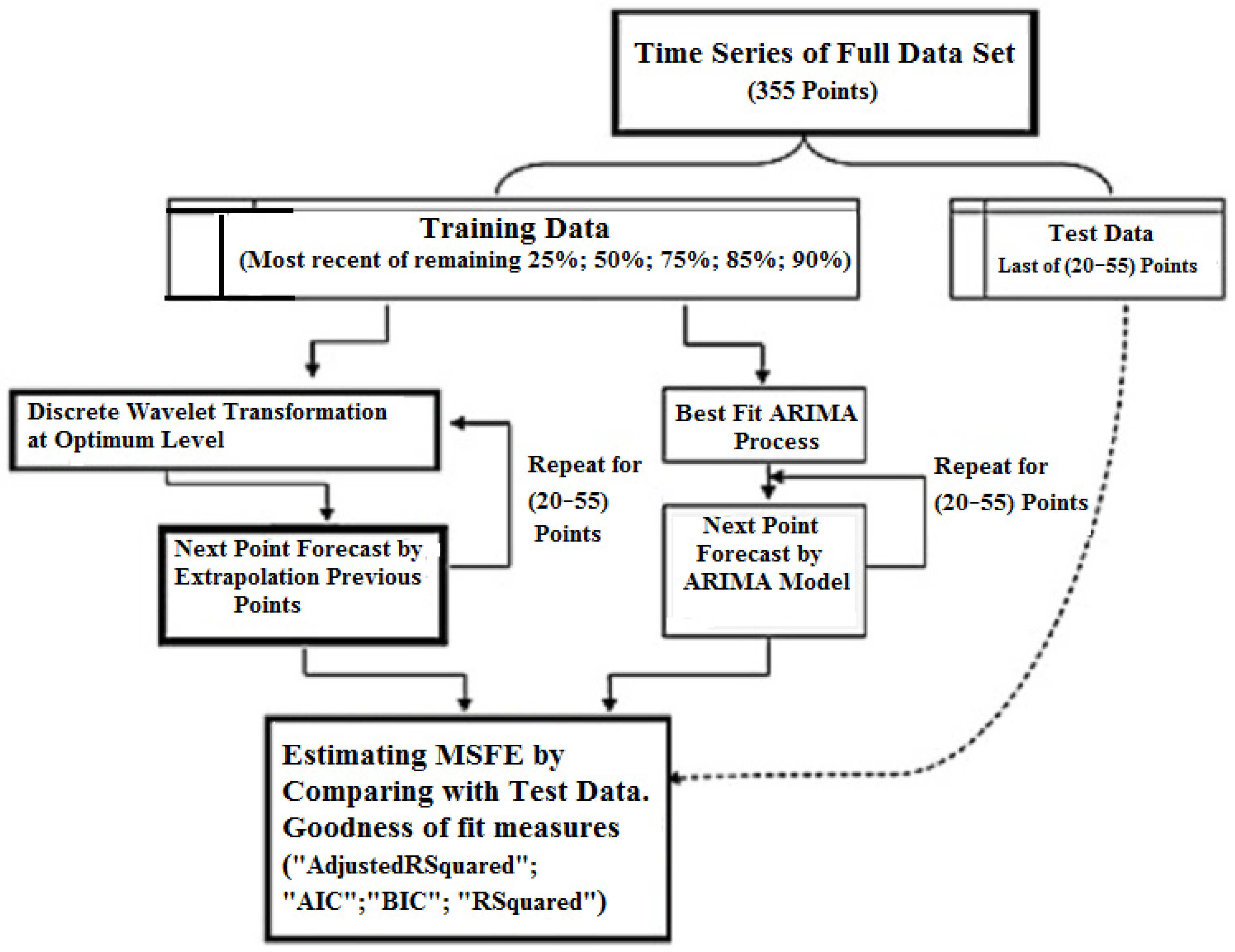
In the present research, the methodology for forecasting the daily remaining balances in the TSA in 2019 using the DWT is based on the approach and analysis of results contained in other works (Yousefi et al. 2005; Atwood et al. n.d.; Merkel 2012).

The general scheme of the modeling stages is shown in Figure 1.

Figure 1. Simulation process flow chart (MSFE: mean squared forecasting error) (the authors’ compilation).

For assessing the quality of the forecasting models, this research utilizes Mean Squared Error (MSE),which includes both dispersion(the range between the predicted values) and shifting (the range between the predicted value y* and its true value y):

$$MSE=\frac{1}{n}{\displaystyle \sum }_{t=1}^{t=n}{\left(y^{*}-y\right)}^2$$

where y* is a predicted value, y is the true value and n is the whole number of values in the test set.

Due to the square term (as shown in the formula above), such a metric fines more for major errors and/or fallouts than for minor errors, which allows one to solve the problem of an extreme value and zero in the indicators of the error absolute values assessment, MAE и MAPE, so this criteria of assessing forecasting models accuracy was chosen.

Comparing the predicted and actual values was conducted on the basis of a linear regression analysis, utilizing the computer system Wolfram Mathematica, Linear Model Fit; for instance: “ANOVA Table”—analysis of variance table; “ANOVA Table Mean Squares”—mean squared errors from the table; “ANOVA Table P Values”—values from the table; “Estimated Variance”—estimate of the error variance; and“Mean Forecasting Errors”—standard errors for the mean forecasting.

Values measuring goodness of fit include:

“Adjusted RSquared”—adjusted for the number of model parameters; “AIC”—the Akaike Information Criterion; “BIC”—the Bayesian Information Criterion; and “RSquared”—the coefficient of determination.

Since a universal indicator of forecasting accuracy does not exist, this research utilizes the MSE indicator, which is especially useful in cases when forecasting value ranges is important.

The forecasting procedure based on the wavelet transform involves four steps: data pre-processing, wavelet decomposition, analysis and the forecasting of signal components upon decomposition, and wavelet reconstruction.

Data pre-processing eliminates inconsistencies and omissions, often associated with certain days (weekends, public holidays, unexpected events, crises, etc.). The approach used in this study provides for the input data smoothing procedure (Wolfram 2022)3, which also gives a reasonable basis for repeated forecasting.

The testable model considered in this research was formed based on the time series dynamics compiled from the daily cash flow balances in the TSA of the federal budget in 2019. In addition, information from the Russian Treasury website was used as input data for the model (The Federal Treasury 2022).

In this article, the statistical analysis and forecasting of the daily balances in the TSA in 2019 were carried out in the following sequential steps (He and Nguyen 2015): (1) downloading the time series data—the balances in the TSA in 2019, presented by months broken down on a basis of working days in the Excel data format; (2) forming the full-time series for 2019, composed based on daily balances in the TSA; and (3) aligning the time series data by taking into account the availability of data for working days only.

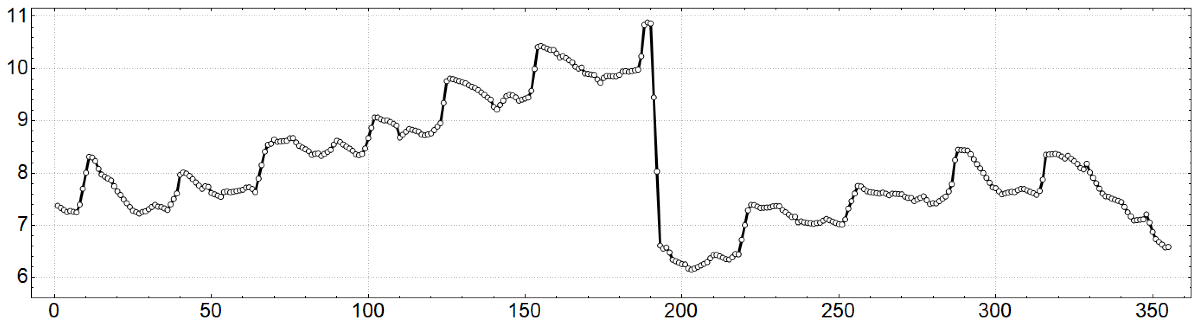
Figure 2 shows the evolution of the time series compiled from the daily remaining balances in the TSA in 2019 (trillion rubles) upon considering the working days in Russia in that year and their further equalization.

Figure 2. Dynamics of daily balances in the TSA in 2019, concerning the time step sequence number, trillion rubles (the authors’ calculations).

In Russia in 2019, there were 254 calendar working days, and as these data were not evenly distributed throughout the year a standard procedure of uniform resampling was used, expressed by applying the Time Series Resample function from the Wolfram Mathematica library, which resulted in receiving 355 points (time steps4), uniformly distributed throughout the year 2019.

Figure 2 shows that the time series compiled from the daily remaining balances in the TSA in 2019 is nonlinear and non-stationary, with more than a 30% decrease at the end of July 2019 and featuring seasonal and noise components.

3. Results and Discussion

Before discussing the results obtained in this study, which allow us to verify if the assumptions expressed in the hypotheses (H1–H3) are true, it is necessary to give certain explanations.

The forecast of the daily balances in the TSA in 2019 was carried out 55 time steps ahead using the DWT approach. The choice of the forecast period was based on the following: (1) the base data for the forecast were limited to one calendar year (355 time steps); and (2) the forecasting power of the wavelet-based forecasting procedure is highly sensitive to the amount of training data. In other words, it works best for large samples of 300 points (time steps) or more. This was confirmed by calculated correlation coefficients between the predicted and the actual values when samples were from 50 to 350 points.

This study developed and examined a model to forecast the daily balances in the TSA in 2019 based on DWT using MW, which belongs to 10 families (Haar, Daubechies, Coiflets, Symlets, Biorthogonal Spline, Reverse Biorthogonal Spline, Meyer, Shannon, Battle-Lemarie and CDF). It is supposed to achieve the research goal and related objectives and confirm or refute the working hypotheses (H1) and (H2), assuming that:

(1) Prior decomposition of the time series compiled from the daily remaining balances in the TSA based on DWT improves the accuracy of traditional forecasting methods;

(2) During the time series decomposition phase, the selection of the mother wavelet function from different wavelet families affects the improvement of forecasting accuracy.

For testing the hypothesis (H3), it was assumed that the time series decomposition level is an important factor affecting forecast accuracy. Therefore, the level number was changed in this study from 1 to 8 to determine the adequate decomposition level, where the mean absolute error wasminimized, and the forecasting accuracy wasimproved.

The obtained results of forecasts based on time series decomposition using the MW belonging to 10 families (Haar, Daubechies, Coiflets, Symlets, Biorthogonal Spline, Reverse Biorthogonal Spline, Meyer, Shannon, Battle-Lemarie and CDF), and adequate statistical tests, are shown in Table 1, Table 2, Table A1, Table A2, Table A3, Table A4, Table A5, Table A6, Table A7, Table A8 and Table A9 and in Figure 3.

Table 1. Families of the wavelet transform and mother wavelet functions were used in the study (the authors’ calculations).

Wavelet Family	Mother Wavelet Function 1	Decomposition Levels
Daubechies	Daubechies Wavelet [1] or Haar Wavelet [] 2; Daubechies Wavelet [2]; Daubechies Wavelet [3]; Daubechies Wavelet [4]; Daubechies Wavelet [5]; Daubechies Wavelet [6]; Daubechies Wavelet [7]; Daubechies Wavelet [8]; Daubechies Wavelet [9]; Daubechies Wavelet [10]; Daubechies Wavelet [12]; Daubechies Wavelet [14]; Daubechies Wavelet [16]; Daubechies Wavelet [18]; Daubechies Wavelet [20].	1, 2, 3, 4, 5, 6, 7, 8
Symlet	Symlet Wavelet [1]; Symlet Wavelet [2]; Symlet Wavelet [3]; Symlet Wavelet [4]; Symlet Wavelet [5]; Symlet Wavelet [6]; Symlet Wavelet [7]; Symlet Wavelet [8]; Symlet Wavelet [9]; Symlet Wavelet [10]; Symlet Wavelet [12]; Symlet Wavelet [14]; Symlet Wavelet [16]; Symlet Wavelet [18]; Symlet Wavelet [20].	1, 2, 3, 4, 6, 8
Coiflet	Coiflet Wavelet [1]; Coiflet Wavelet [2]; Coiflet Wavelet [3]; Coiflet Wavelet [4]; Coiflet Wavelet [5].	1, 2, 3, 4, 5, 6, 7, 8
Biorthogonal Spline	Biorthogonal Spline Wavelet [1.1]; Biorthogonal Spline Wavelet [1.3]; Biorthogonal Spline Wavelet [1.5]; Biorthogonal Spline Wavelet [2.2]; Biorthogonal Spline Wavelet [2.4]; Biorthogonal Spline Wavelet [2.6]; Biorthogonal Spline Wavelet [3.1]; Biorthogonal Spline Wavelet [3.3]; Biorthogonal Spline Wavelet [3.5]; Biorthogonal Spline Wavelet [4.2]; Biorthogonal Spline Wavelet [4.4]; Biorthogonal Spline Wavelet [4.6]; Biorthogonal Spline Wavelet [5.1]; Biorthogonal Spline Wavelet [5.3]; Biorthogonal Spline Wavelet [5.5]; Biorthogonal Spline Wavelet [6.2]; Biorthogonal Spline Wavelet [6.4]; Biorthogonal Spline Wavelet [6.6].	1, 2, 3, 4, 6, 8
Reverse Biorthogonal Spline	Reverse Biorthogonal Spline Wavelet [1.1]; Reverse Biorthogonal Spline Wavelet [1.3]; Reverse Biorthogonal Spline Wavelet [1.5]; Reverse Biorthogonal Spline Wavelet [2.2]; Reverse Biorthogonal Spline Wavelet [2.4]; Reverse Biorthogonal Spline Wavelet [2.6]; Reverse Biorthogonal Spline Wavelet [3.1]; Reverse Biorthogonal Spline Wavelet [3.3]; Reverse Biorthogonal Spline Wavelet [3.5]; Reverse Biorthogonal Spline Wavelet [4.2]; Reverse Biorthogonal Spline Wavelet [4.4]; Reverse Biorthogonal Spline Wavelet [4.6]; Reverse Biorthogonal Spline Wavelet [5.1]; Reverse Biorthogonal Spline Wavelet [5.3]; Reverse Biorthogonal Spline Wavelet [5.5]; Reverse Biorthogonal Spline Wavelet [6.2]; Reverse Biorthogonal Spline Wavelet [6.4]; Reverse Biorthogonal Spline Wavelet [6.6].	1, 2, 3, 4, 6, 8
Meyer	Meyer Wavelet [] 3	1, 2, 3, 4, 5, 6, 7, 8
Shannon	Shannon Wavelet [] 4	1, 2, 3, 4, 5, 6, 7, 8
Battle-Lemarie	Battle-Lemarie Wavelet [1]; Battle-Lemarie Wavelet [2]; Battle-Lemarie Wavelet [3]; Battle-Lemarie Wavelet [4]; Battle-Lemarie Wavelet [5]; Battle-Lemarie Wavelet [6]; Battle-Lemarie Wavelet [7]; Battle-Lemarie Wavelet [8]; Battle-Lemarie Wavelet [9]; Battle-Lemarie Wavelet [10].	1, 2, 3, 4, 5, 6, 7, 8
CDF	CDF Wavelet [9/7]	1, 2, 3, 4, 5, 6, 7, 8

¹ In the Wolfram Mathematica computer-based mathematical system, the wavelets are named after the scientist and a group of scientists who discovered them. However, there are also particular types of wavelets, for example, those with complex functions and stationary and packet wavelets. The wavelet consists of the name of the wavelet, the word “Wavelet” and the wavelet order in square brackets. ² The Wolfram Mathematica computer-based system utilizes Haar Wavelet [], without indicating the order in square brackets, which by default is the Daubechies Wavelet [1]. URL: https://reference.wolfram.com/language/ref/HaarWavelet.html (Accessed on 1 August 2022). ³ In the Wolfram Mathematica computer-based system, the Meyer Wavelet [] without the order indicated inside square brackets is considered the Meyer Wavelet [3] by default. URL: https://reference.wolfram.com/language/ref/MeyerWavelet.html (Accessed on 1 August 2022). ⁴ In the Wolfram Mathematica computer-based system, the Shannon Wavelet [] without the order indicated inside square brackets, which by default belongs to the range {−10, 10}, therefore equals the Shannon Wavelet [10]. URL: https://reference.wolfram.com/language/ref/ShannonWavelet.html (Accessed on 1 August 2022).

Table 2. The result of defining the adequacy of the best forecasting models based on the mother wavelet functions of all the DWT families under analysis (the authors’ calculations).

Wavelet Family	Decomposition Levels	AIC	BIC	Adj-R2	R2
Without time series decomposition/ARIMA	-	−1.528	−7.550	0.78952	0.79341
Without time series decomposition/LSTM RNN	-	−	−	−	0.9590
Haar Wavelet []	-	−42.279	−36.257	0.90739	0.90910
Daubechies Wavelet [8]	8	−102.295	−96.273	0.96610	0.96673
Symlet Wavelet [10]	8	−101.966	−95.944	0.96654	0.96716
Coiflet Wavelet [3]	8	−102.160	−96.138	0.96598	0.96661
Biorthogonal Spline Wavelet [4.4]	8	−102.980	−96.958	0.966581	0.9672
Reverse Biorthogonal Spline Wavelet [5.5]	8	−105.092	−99.0698	0.96895	0.96952
Meyer Wavelet []	5	−99.566	−93.544	0.96508	0.965731
Shannon Wavelet []	1	−103.344	−97.322	0.95919	0.959942
Battle-Lemarie Wavelet [1]	8	−99.1865	−93.165	0.96570	0.966334
CDF Wavelet [9/7]	8	−101.960	−95.939	0.96456	0.965210

Figure 3. Correspondence of forecasted and actual values of balance in the TSA in 2019 (trillions of rub) using the forecasting model upon the eighth iteration of applying the Reverse Biorthogonal Spline Wavelet [5.5], (R² ~ 0.970) (the authors’ calculations).

In order to identify how exactly the selection of the mother wavelet function affects the forecasting accuracy, the paper examined 570 (120 + 90 + 40 + 108 + 108 + 8 + 8 + 80 + 8) forecasting models based on the MW belonging to 10 families (Haar, Daubechies, Coiflets, Symlets, Biorthogonal Spline, Reverse Biorthogonal Spline, Meyer, Shannon, Battle-Lemarie and CDF) (Table 1).

3.1. Verification of Hypotheses (H1)–(H3)

Table A1, Table A2, Table A3, Table A4, Table A5, Table A6, Table A7, Table A8 and Table A9 present the results of tests conducted to evaluate the adequacy of the considered forecasting models for 55 time steps5 to the time series of the values of the daily balances in the TSA 2019, considering all the 570 selected mother wavelet functions and different decomposition levels (from 1 to 8).

The adequacy test included the calculation of the Akaike Information Criterion (AIC) and the Bayesian Information Criterion (BIC) values, as well as the calculation of model accuracy based on the R² coefficient of determination and the adjusted R² coefficient of determination (Adj-RSquared). It should be emphasized that the first row of indicators, shown in Table 2, demonstrates the accuracy of the traditional forecasting model without time series decomposition, which does not exceed 80%.

As defined, the Daubechies Wavelet [1] is equal to the Haar Wavelet []; the Symlet Wavelet [1] is equal to theHaar Wavelet []; the Biorthogonal Spline Wavelet [1,1] is equal to the Haar Wavelet []; and the Reverse Biorthogonal Spline Wavelet [1,1] is equal to the Haar Wavelet []. As follows from Table 2, Table A1, Table A3 and Table A4, the forecast accuracy of the model based on the Haar Wavelet [] slightly exceeds 90%.

3.2. The Influence of the Mother Wavelet Function Selection on the Forecasting Accuracy

3.2.1. The Daubechies Wavelet Family

The selection of the MW from the Daubechies family affected the forecasting accuracy, as shown in Table A1, which demonstrates the results of tests for the adequacy of models based on the MW from the Daubechies family. Table A1 shows that, after ranking the results of the AIC, BIC, R² and Adj-R² criteria, the most favored forecasting model was the one with the prior time series decomposition based on the mother wavelet function (Bogataya et al. 2022), which was the Daubechies Wavelet upon the eighth iteration, characterized by the maximum values of R² = 0.967 and Adj-R² = 0.966 and the minimum values of AIC = −102.295 and BIC = −96.273.

3.2.2. The Symlet Wavelet Family

Regarding the influence of selecting the mother wavelet functions from the Symlet family on the time series forecast accuracy, as shown in Table A2, demonstrating the results of the tests for the adequacy of models based on the MW from the Symlet family, after ranking by the AIC, BIC, R² and Adj-R² criteria, the preferable forecast model was the one with the prior time series decomposition based on the Symlet Wavelet [10] mother wavelet function upon the eighth iteration, characterized by the maximum values of R² = 0.967157 and Adj-R² = 0.966538 and the minimum values of AIC = −101.966 and BIC = −95.944.

3.2.3. The Coiflet Wavelet Family

As shown in Table A3, demonstrating the results of the tests for the adequacy of models based on the MW from the Coiflet family, after ranking by the AIC, BIC, R² and Adj-R² criteria, the preferable forecast model was the one with the prior time series decomposition based on the Coiflet Wavelet [3] mother wavelet function upon the eighth iteration, characterized by the maximum values of R² = 0.967 and Adj-R² = 0.966 and the minimum values of AIC = −102.160 and BIC = −96.138.

3.2.4. The Biorthogonal Spline Wavelet Family

The MW selection from the Biorthogonal Spline family affected the forecasting accuracy, as shown in Table A4. After ranking by the AIC, BIC, R² and Adj-R² criteria, the preferable forecast model was the one with the prior time series decomposition based on the Biorthogonal Spline Wavelet [4.4] mother wavelet function upon the eighth iteration, characterized by the maximum values of R² = 0.9672 and Adj-R² = 0.96658 and the minimum values of AIC = −102.98 and BIC = −96.958.

3.2.5. The Reverse Biorthogonal Spline Wavelet Family

The analysis of the results of the tests for the adequacy of models based on the MW from the Reverse Biorthogonal Spline family is indicated in Table A5. After ranking by the AIC, BIC, R² and Adj-R² criteria, the preferable forecast model was the one with the prior time series decomposition based on the Reverse Biorthogonal Spline Wavelet [5.5] mother wavelet function upon the eighth iteration, characterized by the maximum values of R² = 0.96952 and Adj-R² = 0.96895 and the minimum values of AIC = −105.092 and BIC = −99.0698.

3.2.6. The Meyer Wavelet Family

Table A6 demonstrates the results of the tests for the adequacy of models based on the MW from the Meyer family. After ranking by the AIC, BIC, R², and Adj-R² criteria, the preferable forecast model was the one with the prior time series decomposition based on the Meyer Wavelet [] mother wavelet function upon the fifthiteration, characterized by the maximum values of R² = 0.9657 and Adj-R² = 0.965 and the minimum values of AIC = −99.566 and BIC = −93.544.

3.2.7. The Shannon Wavelet Family

Table A7 demonstrates the results of the tests for the adequacy of models based on the MW from the Shannon family. After ranking by the AIC, BIC, R² and Adj-R² criteria, the preferable forecast model was the one with the prior time series decomposition based on the Shannon Wavelet [] mother wavelet function upon the 1st iteration, characterized by the maximum values of R² = 0.960 and Adj-R² = 0.959 and the minimum values of AIC = −103.344 and BIC = −97.322.

3.2.8. The Battle-Lemarie Wavelet Family

Table A8 demonstrates the results of the tests for the adequacy of models based on the MW from the Battle-Lemarie family. After ranking by the AIC, BIC, R² and Adj-R² criteria, the preferable forecast model was the one with the prior time series decomposition based on the Battle-Lemarie Wavelet [1] mother wavelet function upon the eighth iteration, characterized by the maximum values of R² = 0.966 and Adj-R² = 0.9657 and the minimum values of AIC = −99.187 and BIC = −93.165.

3.2.9. The CDF Wavelet Family

Table A9 demonstrates the results of the tests for the adequacy of models based on the MW from the CDF family. After ranking by the AIC, BIC, R² and Adj-R² criteria, the preferable forecast model was the one with the prior time series decomposition based on the CDF Wavelet [9/7] mother wavelet function upon the eighth iteration, characterized by the maximum values of R² = 0.965 and Adj-R² = 0.9645 and the minimum values of AIC = −101.96 and BIC = −95.939.

Finally, according to the result analysis in Table A1, Table A2, Table A3, Table A4, Table A5, Table A6, Table A7, Table A8 and Table A9, all the analyzed time series decomposition models (based on 570 mother wavelet functions) attained a mean accuracy of over 96% at various decomposition levels. The exceptions wereforecasting models based on the Haar Wavelet [] mother functions, demonstrating accuracy not exceeding 91%. However, their accuracy washigher than the 79% accuracy of the forecasting models without time series decomposition. Upon ranking the AIC and BIC and by the R² and Adj-R² criteria, the best time series decomposition models based on the mother wavelet function were selected from each wavelet family (Table 2).

Additionally, in Table 2, among the forecasting models without wavelet decomposition, besides the linear ARIMA model, the accuracy (R²) of a nonlinear forecasting model based on a 10-layer recurrent neural network, LSTM (Long Short-Term Memory) RNN (Recurrent Neural Network), trained on data reflecting the budget balance dynamics in the accounts of TSA for 300 training rounds, is presented. As can be seen from Table 2, the accuracy of the nonlinear LSTM RNN model (R² = 0.9590) without decomposition is inferior to all forecasting models with decomposition based on wavelet transforms. An exception is a model based on decomposition of the Haar Wavelet [] (R² = 0.9091), indicating a large forecasting potential of the forecasting models based on raw data decomposition using wavelet transforms.

As shown in Table 2, the highest forecasting accuracy was achieved for the time series decomposition model based on the mother wavelet function Reverse Biorthogonal Spline Wavelet [5.5] upon eight iterations (AIC = −105.092; BIC = −99.0698; Adj R² = 0.968945; R² = 0.96952).

Moreover, Table 2 shows therankings of the first three forecasting models that compete in accuracy by the R² and Adj-R² criteria, considering various mother wavelet functions and various decomposition level values, resulting in the following order:

The first place was the forecasting model based on the mother function Reverse Biorthogonal Spline Wavelet [5.5] after eight iterations: R² = 0.96952; Adj-R² = 0.96895;

The second place was the forecasting model based on the mother function Biorthogonal Spline Wavelet [4.4] after eight iterations: R² = 0.9672; Adj-R² = 0.966581;

The third place was the forecasting model based on the mother function Symlet Wavelet [10] after eight iterations: R² = 0.96716; Adj-R² = 0.96654.

Ranking the first three forecasting models competing in information tests by the AIC and BIC, considering various mother wavelet functions and various decomposition level values, results in the following order:

The first place was the forecasting model based on the mother function Reverse Biorthogonal Spline Wavelet [5.5] after eight iterations: AIC = −105.092; BIC = −99.0698;

The second place was the forecasting model based on the mother function Shannon Wavelet [] after one iteration: AIC = −103.344; BIC = −97.322;

The third place was the forecasting model based on the mother function Biorthogonal Spline Wavelet [4.4] after eight iterations: AIC = −102.980; BIC = −96.958.

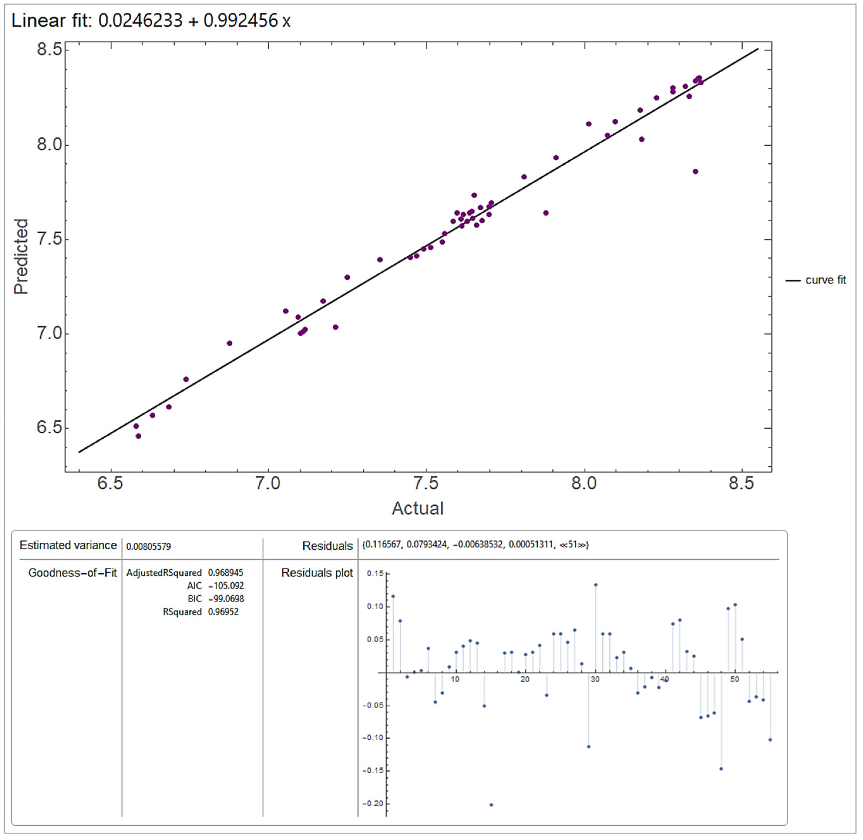
As a result of comparative analysis, the most competitive forecasting model in all the tests (AIC, BIC, Adj-R² and R²) was the forecasting model based on the mother function Reverse Biorthogonal Spline Wavelet [5.5] after eight iterations (AIC = −105.092; BIC = −99.0698; Adj R² = 0.968945; R2 = 0.96952; ANOVA Table Mean Squares = {13.5807, 0.00805579}; Estimated Variance = 0.00805579).

Figure 3 shows the compliance of the forecasted values with the actual values of the balance in the TSA in 2019 (trillions of rub) when using the forecasting model upon the eighth iteration of applying the Reverse Biorthogonal Spline Wavelet [5.5].

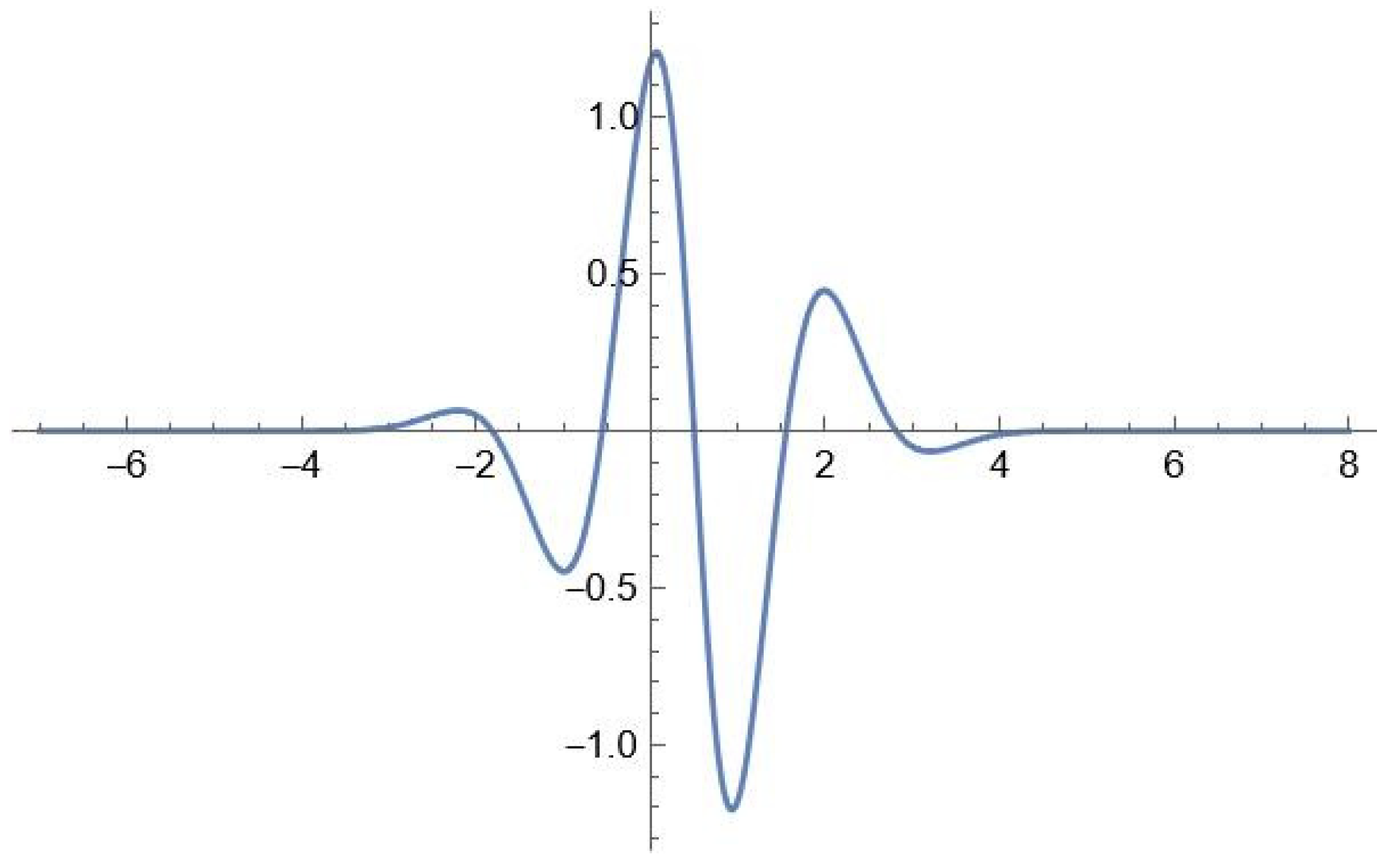
Figure 4 presents, for clarity, a graph of the mother wavelet function Reverse Biorthogonal Spline Wavelet [5.5], which generally repeats the overall graph contours of the changing time series graph composed of the TSA budget balances in 2019 (Figure 2).

Figure 4. Graph of mother wavelet function Reverse Biorthogonal Spline Wavelet [5.5] (the authors’ calculations).

According to this study’s results, the time series decomposition model based on the Reverse Biorthogonal Spline Wavelet [5.5] mother wavelet function upon eight iterations is recognized as the best one (in terms of forecasted value compliance with the actual values of the time series) with a sample of 570 mother wavelet functions. The high accuracy of the forecasting model based on the Reverse Biorthogonal Spline Wavelet [5.5] mother wavelet function upon eight iterations arises from the fact that the desired properties for decomposition and reconstruction are separated for the biorthogonal dyadic wavelets with a compact carrier. Thisis the determining factor in solving the problem of increasing the accuracy of the time series compiled from the daily balances in the TSA at the prior decomposition stage.

3.3. Verifying Hypotheses (H1)–(H3) (Testing Results for Hypotheses (H1)–(H3)

The modeling results in Table 2, Table A1, Table A2, Table A3, Table A4, Table A5, Table A6, Table A7, Table A8 and Table A9 demonstrate that the modeling forecasts of the time series compiled from the daily balances in the TSA in 2019, using the time series decomposition based on the MW from 10 families and considering1–8 decomposition levels, based on the 300-point sample and 55time steps, demonstrate fairly high accuracy (over 96%). This indicates that the research goal was achieved, and that the hypotheses (H1) and (H2) are true for the prior times series decomposition based on the Reverse Biorthogonal Spline Wavelet [5.5] MW, which contributes to achieving a forecasting accuracy of over 97%, whereasit is only possible to reach around 80% accuracy without decomposition.

Regarding hypothesis H3, Table 2, Table A1, Table A2, Table A3, Table A4, Table A5, Table A6, Table A7, Table A8 and Table A9 show that the decomposition level significantly influences the forecast accuracy regardless of the MW. Thisis because a higher decomposition level provides a more comprehensive picture of the time series data. However, it may also generate redundancy of features and noise, which can lead to an increase in computational cost and a decrease in the classification characteristics of the analyzed time series.

4. Conclusions

In this research, three scientific hypotheses were formulated to solve the problem of improving forecasting accuracy for a time series composed of daily cash flow balances in the federal budget TSA. The research results fully confirm the validity of all three hypotheses. The preliminary decomposition of the time series (H1), based on the DWT (H2), improves the accuracy of traditional forecasting methods, and the number of time series decomposition levels is an important factor, affecting the forecasting accuracy (H3).

Summarizing the results obtained in this study, we can emphasize that the procedure of prior decomposition based on the DWT of a non-stationary, nonlinear time series compiled from the daily balances in the TSA contributes to a significant accuracy increase (from 80% to 97%) for the traditional methods of time series forecasting. The study examines the influence of selecting a mother wavelet out of 570 mother wavelet functions belonging to 10 wavelet families (Haar, Dabeshies, Symlet, Coiflet, Biorthogonal Spline, Reverse Biorthogonal Spline, Meyer, Shannon, Battle-Lemarie and CDF) and the decomposition level (from 1 to 8) on the forecasting accuracy by the Akaike and the Bayesian information criteria (AIC and BIC) and the coefficient of determination (R² and Adj-R²).

The modeling results show that the time series forecasting model based on the Reverse Biorthogonal Spline Wavelet [5.5] mother wavelet function features the highest accuracy of all the 570 forecasting models reviewed. It should be noted that the mother wavelet functions belonging to the family of reverse biorthogonal spline wavelets are symmetric, with a compact carrier. Therefore, the parameters for decomposition and reconstruction are separated, which is the determining factor in solving the problem of increasing the accuracy of the time series compiled from the daily balances in the TSA at the prior decomposition stage.

This paper determines that various forecasting models are sensitive to the level of decomposition regardless of the selected MW.

The study results demonstrate that the choice of the MW and the decomposition level play an important role in increasing the accuracy of forecasting the daily balances in the TSA.

The novelty of this study is that the procedure of prior decomposition based on the DWT of non-stationary, nonlinear time series compiled from the daily balances in the TSA is effective when solving the problem of improving the accuracy of traditional forecasting methods.

The theoretical significance of the results is determined by the fact that they provide direction for improving the forecasting accuracy of traditional methods of forecasting nonlinear, non-stationary time series, demonstrating the significant forecasting potential of methods with prior decomposition based on the DWT.

The practical significance of the obtained results is determined by the proven fact of the selected mother wavelet functions from 10 wavelet families (Haar, Daubechies, Coiflets, Symlets, Biorthogonal Spline, Reverse Biorthogonal Spline, Meyer, Shannon, Battle-Lemarie and CDF) affecting the accuracy of models forecasting the balances remaining in the TSA. The latter is particularly interesting to treasurers, cash managers and money managers, who can use the cash more efficiently by relying on more accurate cash flow forecasts.

Despite the significant results obtained, it is necessary to note certain constraints in addition to the conclusions drawn.

In this study, the mother wavelet functions belonging to 10 families (Haar, Daubechies, Coiflets, Symlets, Biorthogonal Spline, Reverse Biorthogonal Spline, Meyer, Shannon, Battle-Lemarie and CDF) were used at the time series decomposition stage. In addition, the traditional methods based on regression equation extrapolation were also used at the forecasting stage.

In future studies, the forecasting methods may involve using artificial intelligence, machine learning and neural networks with deep learning, which, together with wavelet decomposition, can further increase the accuracy and relevance of cash flow forecasts.

Considering the undoubted success in analyzing and forecasting the complex behavior of objects described with nonlinear, non-stationary time series, hybrid methods based on wavelet transformations and linear models MODWT-ARMA/ARIMA/SARIMA (Zhu et al. 2014), as well as artificial neural networks MODWT-NN/EWEnet (Panja et al. 2022), the future research of the authors will analyze hybrid forecasting methods based on technologies of artificial intelligence, machine learning and neural networks with deep learning, which can be combined with wavelet decomposition and can further increase the accuracy as well as, undoubtedly, the practical value of monetary flow forecasting.

References

- Antonopoulou, Hera, Vicky Mamalougou, and Leonidas Theodorakopoulos. 2022. The role of economic policy uncertainty in predicting stock return volatility in the banking industry: A big data analysis. Emerging Science Journal 6: 569–77. [Google Scholar] [CrossRef]
- Atwood, Bruce, Caroline Haddad, Helmut Knaust, and John Merkel. n.d. Using Wavelets-Based Time Series Forecasting to Predict Oil Prices. Wavelets in Undergraduate Education. Available online: http://helmut.knaust.info/presentations/2012/20120106_JMM/Haddad%20(not%20final).pdf (accessed on 12 March 2022).
- Bogataya, Irina, Elena Evstafyeva, Denis Lavrov, Ekaterina Korsakova, Natalya Mukhanova, and Svetlana Solyannikova. 2022. Disclosure of information in risk reporting in the context of the sustainable development concept. Sustainability 14: 2300. [Google Scholar] [CrossRef]
- Cangoz, M. Coskun, and Leandro Secunho. 2020. Cash Management—How Do Countries Perform Sound Practices? Equitable Growth, Finance, and Institutions Insight. Washington, DC: The World Bank. [Google Scholar]
- Chi, Dianwei. 2022. Research on electricity consumption forecasting model based on wavelet transform and multi-layer LSTM model. Energy Reports 8: 220–28. [Google Scholar] [CrossRef]
- Daubechies, Ingrid. 1992. Ten Lectures on Wavelets. Philadelphia: Society for Industrial and Applied Mathematics (SIAM), Volume 61. [Google Scholar]
- Donskikh, Oleg A. 2019. Horror zivilisationis, or the horror of subjectivity. The Beacon: Journal for Studying Ideologies and Mental Dimensions 2: 020110205. [Google Scholar] [CrossRef]
- Dyakonov, Vladimir. 2012. Wavelets in СКМ Mathematica 8. Components and Technologies 9: 145–52. [Google Scholar]
- Fry, John, Vlad-Marius Griguta, Luciano Gerber, Helen Slater-Petty, and Keeley Crockett. 2021. Modelling corporate bank accounts. Economics Letters 205: 109924. [Google Scholar] [CrossRef]
- Gencay, Ramazan. 2002. An Introduction to Wavelets and Other Filtering Methods in Finance and Economics. New York: Academic Press. [Google Scholar]
- He, Tian-Xiao, and Tung Nguyen. 2015. Wavelet analysis and applications in economics and finance. Research & Reviews: Journal of Statistics and Mathematical Sciences 1: 22–37. [Google Scholar]
- Ibrahim, Izani, Kamilah Kamaludin, and Sheela Sundarasen. 2020. COVID-19, government response, and market volatility: Evidence from the Asia-Pacific developed and developing markets. Economies 8: 105. [Google Scholar] [CrossRef]
- Iskandar, Iskandar. 2019. The Development of Government Cash Forecasting Model: A Case Study for the Indonesian Government. Ph.D. thesis, University of Tasmania, Tasmania, Australia. [Google Scholar]
- Iskandar, Iskandar, Roger Willett, and Shuxiang Xu. 2018. The development of a government cash-forecasting model. Journal of Public Budgeting, Accounting & Financial Management 30: 368–83. [Google Scholar]
- Journeys to Treasury. 2021. Striving for the Summits of Treasury with BNP PARIBAS—EACT—PwC—SAP. Available online: https://cmcc.bnpparibas.com/hubfs/Journeys%20to%20Treasury%202020/Journeys%20to%20Treasury%202020-2021%20read.pdf (accessed on 12 March 2022).
- Kutsuri, Georgiy N., Lola D. Sanginova, and Svetlana S. Galazova. 2020. Warranties of public-law entity as a type of debt obligation in a systemic economy. Lecture Notes in Networks and Systems 129: 1094–101. [Google Scholar]
- Lienert, Ian. 2009. Modernizing Cash Management. Technical Notes and Manuals. International Monetary Fund. Available online: https://www.imf.org/external/pubs/ft/tnm/2009/tnm0903.pdf (accessed on 12 March 2022).
- Liu, Kailei, Jinhua Cheng, and Jiahui Yi. 2022. Copper price forecasted by a hybrid neural network with Bayesian optimization and wavelet transform. Resources Policy 75: 102520. [Google Scholar] [CrossRef]
- Malekpour Heydari, Salimeh, The Noranis Mohd Aris, Razali Yaakob, and Hazlina Hamdan. 2021. Data-driven forecasting and modeling of runoff flow to reduce flood risk using a novel hybrid wavelet-neural network based on feature extraction. Sustainability 13: 11537. [Google Scholar] [CrossRef]
- Mallat, Stephane. 1999. Wavelet Tour of Signal Processing. Amsterdam: Elsevier. [Google Scholar]
- Manetti, Alessandro, Antonia Ferrer-Sapena, Enrique A. Sánchez-Pérez, and Pablo Lara-Navarra. 2021. Design trend forecasting by combining conceptual analysis and semantic projections: New tools for open innovation. Journal of Open Innovation: Technology, Market, and Complexity 7: 92. [Google Scholar] [CrossRef]
- Merkel, John. 2012. Undergraduate Research Projects on Wavelet-Based Time Series Forecasting. Atlanta: Oglethorpe University. [Google Scholar]
- Moskovkin, Vladimir M. 2020. Do we need a Great Reset? COVID-19, Black Revolution, inequality and common good. The Beacon: Journal for Studying Ideologies and Mental Dimensions 3: 011310115. [Google Scholar] [CrossRef]
- Panja, Madhurima, Chakraborty Tanujit, Kumar Uttam, and Liu Nan. 2022. Epicasting: An Ensemble Wavelet Neural Network (EWNet) for Forecasting Epidemics. arXiv arXiv:2206.10696. [Google Scholar]
- Parvini, Navid, Mahsa Abdollahi, Sattar Seifollahi, and Davood Ahmadian. 2022. Forecasting bitcoin returns with long short-term memory networks and wavelet decomposition: A comparison of several market determinants. Applied Soft Computing 121: 108707. [Google Scholar] [CrossRef]
- Pattanayak, Sailendra, and Israel Fainboim. 2010. Treasury Single Account: Concept, Design, and Implementation Issues. International Monetary Fund. Available online: https://www.imf.org/external/pubs/ft/wp/2010/wp10143.pdf (accessed on 12 March 2022).
- Peng, Lu, Lin Wang, De Xia, and Qinglu Gao. 2022. Effective energy consumption forecasting using empirical wavelet transform and long short-term memory. Energy 238: 121756. [Google Scholar] [CrossRef]
- Percival, Donald B., and Andrew T. Walden. 2006. Wavelet Methods for Time Series Analysis. Cambridge: Cambridge University Press, vol. 4. [Google Scholar]
- Percival, Donald B., Muyin Wang, and James E. Overland. 2004. An introduction to wavelet analysis with applications to vegetation time series. Community Ecology 5: 19–30. [Google Scholar] [CrossRef]
- Semenova, E. A. 2021. Liquidity Management and Cash Flow Forecasting in the Context of the Epidemiological Crisis. Moscow: N.A. Publisher. [Google Scholar]
- Shaikh, Wajid Ali, Feroz Shah Syed, Siraj Muhammed Pandhiani, and Muhammad Anwar Solangi. 2022. Wavelet decomposition impacts on traditional forecasting time series models. Computer Modeling in Engineering & Sciences 130: 1517–32. [Google Scholar]
- Storkey & Co Limited. 2001. International Government Cash Management Practices. Available online: https://storkeyandco.com/files/1213/8731/5474/International_Cash_Management_Practices.pdf (accessed on 12 March 2022).
- Sumando, Eko, Fidia Dwi Hamiyani, and Irwan Diko Purba. 2018. Pengembangan Metode Cash Forecasting Pemerintah: Studi Kasus Saldo Kas Pemerintah 2009–2011. Kajian Ekonomi & Keuangan 2: 70–93. [Google Scholar]
- The Federal Treasury. 2022. Financial Transactions. Available online: https://roskazna.gov.ru/finansovye-operacii (accessed on 13 June 2022).
- Torrence, Christopher, and Gilbert P. Compo. 1998. A practical guide to wavelet analysis. Bulletin of the American Meteorological Society 79: 61–78. [Google Scholar] [CrossRef]
- Van Fleet, Patrick J. 2019. Discrete Wavelet Transformations: An Elementary Approach with Applications, 2nd ed. Hoboken: Wiley. [Google Scholar]
- Vidakovic, Brani. 1999. Statistical Modeling by Wavelets. New York: John Wiley & Sons. [Google Scholar]
- Vogl, Markus, Peter Gordon Rötzel LL. M., and Stefan Homes. 2022. Forecasting performance of wavelet neural networks and other neural network topologies: A comparative study based on financial market data sets. Machine Learning with Applications 8: 100302. [Google Scholar] [CrossRef]
- Williams, Mike. 2004. Government Cash Management: Good and Bad Practice. Available online: http://www.mj-w.net/cac_gov_cash.html (accessed on 22 August 2021).
- Williams, Mike. 2010. Government Cash Management: Its Interaction with Other Financial Policies. International Monetary Fund. Available online: https://www.imf.org/external/pubs/ft/tnm/2010/tnm1013.pdf (accessed on 12 March 2022).
- Wolfram. 2022. Wavelet Analysis. Available online: https://reference.wolfram.com/language/guide/Wavelets.html (accessed on 12 March 2022).
- Yousefi, Shahriar, Ilona Weinreich, and Dominik Reinarz. 2005. Wavelet-basedforecastingofoilprices. Chaos, Solitons & Fractals 25: 265–75. [Google Scholar]
- Zhang, Xin, Donggyu Kim, and Yazhen Wang. 2016. Jump variation estimation with noisy high-frequency financial data via wavelets. Econometrics 4: 34. [Google Scholar] [CrossRef]
- Zhu, Li, Wang Yanxin, and Fan Qibin. 2014. MODWT-ARMA model for time series forecasting. Applied Mathematical Modelling 38: 1859–65. [Google Scholar] [CrossRef]
Publisher’s Note: MDPI stays neutral with regard to jurisdictional claims in published maps and institutional affiliations. |
© 2022 by the authors. Licensee MDPI, Basel, Switzerland. This article is an open access article distributed under the terms and conditions of the Creative Commons Attribution (CC BY) license (https://creativecommons.org/licenses/by/4.0/).