1. Introduction
One of the hallmarks of the COVID-19 pandemic is uncertainty. As the outbreak progressed and the economy evolved, decisionmakers needed tools that described up-to date, current realities as they occurred. It was well understood that the economy was in a massive state of upheaval, but—precisely how massive? What were the state-by-state differences and similarities? What was happening in different sectors of the economy? The same is necessarily true of the economic recovery. Having ways to model what arises is critical to creating quality policy plans that address targeted issues. Data must be comprehensive enough to cover many potential futures, flexible enough to apply to different parts of society, and clear enough to accurately describe the potential impacts from policy decisions. The approach presented in this paper creates a new set of tools that provide a view of the economy using current data, facilitates rapid model generation in the present landscape, and then presents limited use cases to demonstrate the impacts using a “Multi-Level Nowcast” methodology. This allows for a current-state, quality evaluation of economic ramifications, given that non-pandemic past recessions are suboptimal datasets on which to model.
Researchers have devised a variety of ways to evaluate the economic landscape after the advent of COVID-19, albeit with significant shortcomings to each approach. Many researchers turned to the U.S. census’ American Community Survey for guidance in the early months of COVID-19; however, data collected were two to three years old (
Kaiser Family Foundation 2020;
Leibovici et al. 2020). In a study published by the University of Chicago, researchers studied data from a private company that revealed dramatic drops in the number of hourly employees working and total hours worked, along with increases in firm shutdowns (
Bartik et al. 2020). Other University of Chicago economists used cellphone data to track customer visits to over 2.25 million businesses, finding that consumer traffic dropped more than 60 percent during the lockdown (
Goolsbee and Syverson 2020). While Unemployment Insurance claims (UI) are one of the few just-in-time indicators of the job market in America, they are not useful for predicting policy effects on target populations, since only a portion of the workforce qualifies for UI in the event of job loss. Data in the aforementioned studies have multi-level aspects, but each has the drawback of being either proprietary data, a fractional portion of the overall U.S. picture, or information that is badly outdated. In short, better approaches are needed to answer real-time questions.
This paper seeks to address structural gaps in the data highlighted above by using raw data from the Bureau of Labor Statistics (BLS) and manipulating it to create a “Multi-Level Nowcast”. As a useful example, the current-state Nowcast is then used to evaluate the impacts of airline industry losses on Colorado’s economy and Arizona’s economy and then discuss the differences between the two. Impacts of the COVID-19 induced recession on low-wage employees are then considered, using the same basic dataset. One great advantage of this approach is, of course, that the raw data and spreadsheet processing software are publicly available and free—so the method is quite available to interested researchers. In that sense, the ultimate goal of this paper is to create a practical, simple, and costless approach for non-experts to create a viable Nowcast for planning purposes.
Section 2 provides a brief evaluation of the broader impacts the airline industry has on state economies, as well as more detailed motivations for our particular interest in this topic of study. While this paper uses airline industry employment to illustrate how a Multi-Level Nowcast can be used, the approach can be expanded to study any area supported by the underlying BLS datasets. Since this encompasses diversity in geographies, industries, and income levels, the approach provides a very flexible framework for future investigations.
Section 3 presents analytical results of findings, with
Section 4 offering conclusions.
Appendix A provides more details regarding standard accuracy criteria and an evaluation of Nowcasting compared to statistical ARIMA model results.
Appendix B discusses AR-X incompatibility with the Nowcasting used in this publication. Finally, for those interested in creating their own Multi-Level Nowcast,
Appendix C and
Appendix D offer detailed instructions.
The steps in creating a Multi-Level Nowcast are detailed but not difficult, with illustrations of both the process and actual datasets to assist in the replication of the methodology for future researchers.
Without a Nowcast there is no current, detailed framework of publicly available data from which to model current and future shocks, either by job title or income level. As COVID-19 continues to change America’s economic landscape, having a universal practical framework that allows for flexible, targeted cuts of the economy is a very powerful tool. Information from the Nowcast can also be used as a foundation for other investigations and is not a final, singular output. Creating a Nowcast allows a researcher to quickly model how impacts—whether based in policy or economic trends—are expected to affect those within the area of interest.
2. Materials and Methods
Recognizing the need for a near-term data solution, several leading institutions and scholars were quick to estimate closer-to-real-time estimates of various economic phenomena. The NY Fed Nowcast, the Weekly Economic Indicator (
Lewis et al. 2020), and countless non-traditional data sources were used, including changes to employee hours worked (
Bartik et al. 2020), restaurant reservations (
Lewis et al. 2020), and travel-based data, such as hotel occupancy rates (
STR 2020) and daily TSA screenings. All showed dramatic changes happening in near real time, but none were capable of showing the immediate pressure on low-wage workers.
In mid-April of 2020,
Parolin and Wimer (
2020) estimated the possible extent of suffering among the U.S. population, as a whole, should the unemployment rate remain around 30 percent through 2020—forecasting an increase in the poverty rate from 12.4 to 18.9 percent (or more than 21 million people). Granted, 30 percent unemployment was not sustained through 2020, and forecasting possible unemployment trajectories is notably difficult, as discussed in
Petrosky-Nadeau and Valletta (
2020). Although poverty estimates are presented on an annual basis and with a considerable lag, the
Parolin and Wimer (
2020) report was timely, receiving considerable media coverage. Nonetheless, geographically specific data on low-wage workers and an up-to-date industry-specific investigation remained elusive. The methodology in this paper seeks to solve that problem.
Given the broad potential applications and pressing need, a solution that augments publicly available data and closes the data gap without reliance on proprietary tools or methods is needed. Although much of the private data listed above were beneficial and timely, there is no guarantee such data will always be available. Further, as private, proprietary data, the quality and veracity of the information cannot be validated or crosschecked by other researchers. Not only is the BLS data public, but it is also high-quality. The Quarterly Census of Employment and Wages (QCEW) is the most comprehensive source of data on employment, hours, and wages by industry in the U.S., covering about 97 percent of all civilian wages and salaries. The data are available at the national, state, metropolitan area, and county levels. The BLS’s Current Employment Statistics (CES) are similarly considered a “gold standard”—one of the most timely and sensitive datasets published by the federal government. The CES sample is drawn from the QCEW, using the more than 10 million establishments covered by unemployment insurance. Although neither covers certain agricultural workers, the self-employed, or unpaid family workers, the CES does include certain jobs not covered by UI, including railroad jobs and those in religious organizations. Additionally, the two data sources trend well together.
Another valuable reason to use BLS data is that so many stakeholders rely on it. The data are widely understood, structurally stable, and well supported within federal budgets. Policymakers rely on the BLS to inform debates around healthcare, social security, and employee benefits, but private industry also uses several BLS sources quite heavily. Having a high-quality, neutral dataset that allows for comparisons of compensation and benefits across different industries, occupations, and regions is advantageous for so many groups that users of all stripes have a vested interest in retaining quality, continuous BLS datasets. Selecting this particular public data source for study provides a high degree of certainty regarding future data quality and accessibility.
Importantly, the use of the specific public datasets selected makes analyses applicable in each individual state, allowing for replicability and comparison when evaluating unfolding trends. States, of course, are often responsible for implementing social service programs that individuals and families rely upon when economic shocks occur. Fiscal changes made at the federal level filter through each state in different ways, so real-time data are essential for state-level policymakers to make informed decisions—decisions that often require considerable amounts of public resources.
2.1. Operational Example—Near-Term Nowcasting for the Airline Industry
The airline industry was chosen as an example in this paper for a few reasons. Firstly, the industry is highly susceptible to demand shocks. The beginning of the 1980s and 1990s, 2001–2005, and post-2008 were all periods of significant losses in terms of employment and profits. All of these shocks pale in comparison to the initial losses experienced due to COVID-19. The UN agency for civil aviation has estimated that global financial losses to airlines and airports totaled USD 370 billion and USD 115 billion, respectively, in 2020 (
ICAO 2021). For North America alone, gross airline passenger operating revenues dropped USD 88 billion, while airport revenues dropped over USD 22 billion.
Secondly, the airline industry is highly geographically concentrated due to airport hubs. Pushing the maximum amount of traffic through a hub is beneficial both to airline companies, due to lower overhead costs, as well as to passengers, due to greater choices in flight availability and costs, a topic nicely summarized in
Button and Lall (
1999). Hubs are also beneficial to their surrounding areas.
McGraw (
2016) found that hub airports increase personal income and establishment counts in their commuting zones by 2.3 and 1.6 percent, respectively. An ancillary effect is that many companies intentionally choose to locate in areas near airport hubs. This is particularly true for wholesale trade and distribution centers. Thus, an economic downturn in air traffic can have considerable negative impacts.
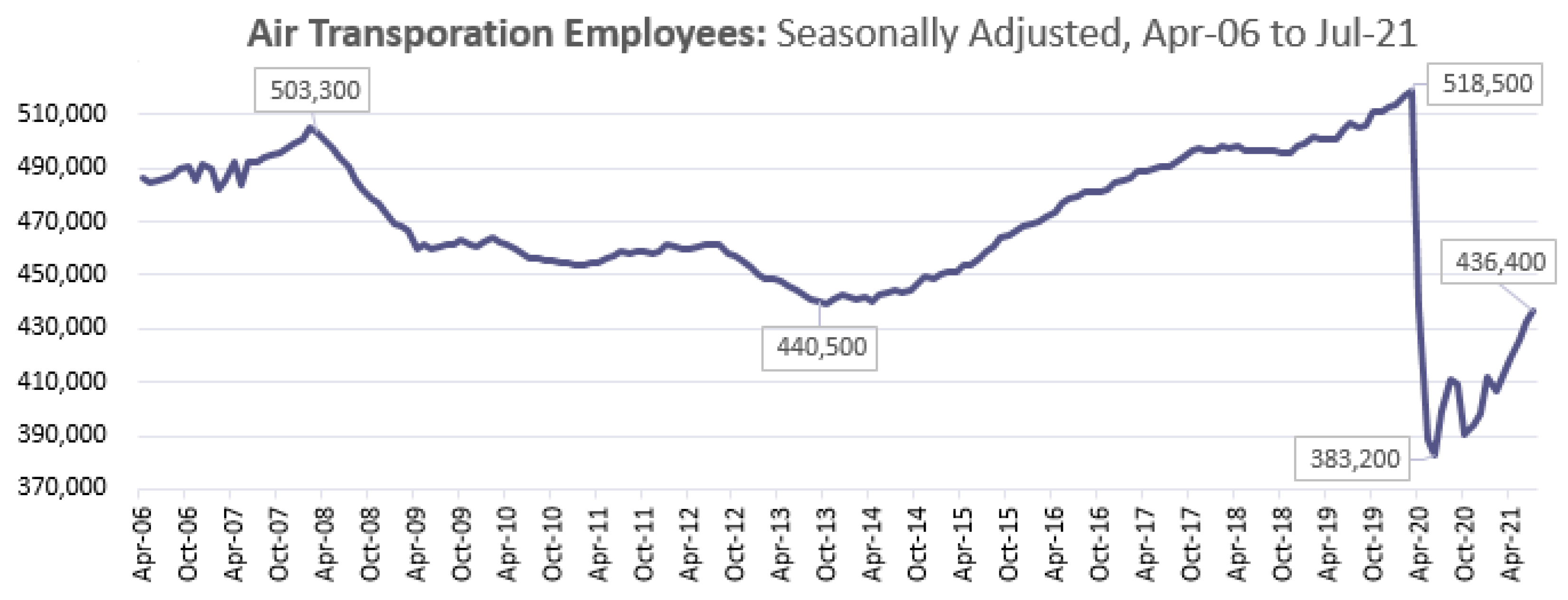
Lastly, and crucial to this paper, the airline industry is highly segmented. There are airport personnel with middle to high incomes—including those responsible for flight operations, engineering and maintenance, and sales and marketing—a large majority of whom belong to a union. There is also a considerable workforce that is subcontracted by the major airlines—including food service, airport security, cleaning, and fueling—who frequently earn low wages and are rarely covered by collective bargaining agreements. COVID-19 impacted airline workers in different ways. Whereas schedule changes imposed by the FAA on the country’s air traffic control system caused some disruption to air traffic controllers, a number of airline companies underwent major furloughs and layoffs. Nationally, air transportation employment alone dropped over 130,000 from January to June of 2020, as shown in
Figure 1 (
U.S. Bureau of Labor Statistics 2021).
2.2. Regional Detail—The U.S. States of Colorado and Arizona Show the Airline Industry Example
Within the United States, and particularly within the Mountain West Region, Colorado and Arizona present unique cases for evaluating economic trends. As two states without coastal components of their economy, both Colorado and Arizona have been among the most successful economies nationwide and have experienced a high rate of growth as well as economic diversification over time. They are the top two states in terms of employment for the Region, as shown by the upper lines on the graph, yet adequately proxy patterns seen in the remaining states within the Mountain West, particularly in terms of the Region’s year-over-year employment changes (
Figure 2). In both states, rural/urban patterns are very similar, and employment growth over the past 14 years has followed similar trajectories.
With its central geographical placement, Colorado has long been an airline hub and an important location for both travelers and transit alike. Considering the proportion of jobs in the state that are supported by the airline industry, Colorado has the second highest percentage in the Mountain West, trailing only Nevada in its percentage impact on the overall economy. Colorado’s evaluation comes in contrast to Arizona, which has airline employment patterns that more closely reflect typical patterns within the Region. Minor carriers have experimented with placing more hub operations in Arizona, and overall employment numbers are very similar to Colorado’s, but the percentage of employment has not occurred on the scale of Colorado’s legacy of airline operations. Using two such similar economies, yet with very different airline employment patterns, provides an interesting vantage point from which to evaluate broad economic trends.
2.3. Robustness
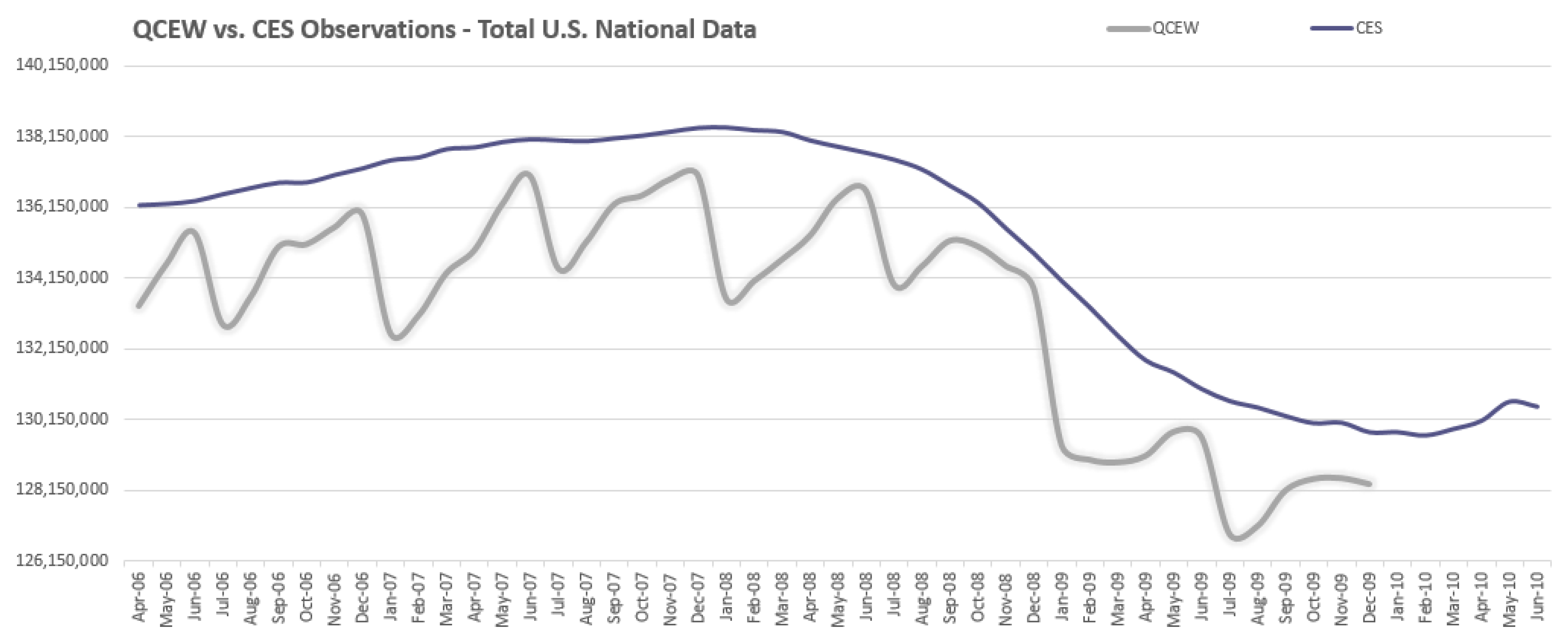
When taking such an unusual approach to BLS data, it was important to evaluate the appropriateness of the methodology described below. Although the CES and QCEW come from a similar universe, the total employment counts for each differ, as each excludes certain types of jobs. The CES reports more jobs than the QCEW because the CES covers many jobs that are not present in the QCEW. For example, while both CES and QCEW include state government education jobs, the CES picks up students employed through Work Study while the QCEW does not. Nevertheless, the two series track well together, even during volatile periods, such as the Great Recession. During this timeframe, the CES data were consistently above final QCEW data (at the end of all government-run updates) and mostly within a margin of 0.7–3.6% of the final QCEW values, as shown in
Figure 3. In other words, the QCEW was always within 4 percentage points of the CES on any given month throughout the Great Recession. Very importantly, the CES data presaged rise and drop, something that was later validated by the final QCEW publications. And without inserting the CES data, researchers would be left without anything to evaluate until QCEW data are finally released. Creating a Nowcast by meshing QCEW + CES datasets allows researchers to do a much better job of understanding what is occurring, even in the midst of upheaval, than if this tool were unavailable.
For the test cases presented in this paper, the Nowcast methodology uses CES data to bring current the overall view of the economy, with older CES data being replaced as QCEW reports become available. Yet the CES data still serve the same function as they do nationally: they catch the direction and magnitude of final QCEW data. During the same time period as the Great Recession, shown in
Figure 3 above, Colorado’s portion of CES data was within a margin of 0.8% below or 4.2% above final QCEW values, with both median and average differences from the CES being just 1.5% more than the final QCEW data. The same trend held for Colorado as for the national data: the CES correctly reflected the inflection points and magnitude of changes shown in the final QCEW information.
While the CES provides useful U.S. employment data and is quite current, showing data for the immediately preceding month, the QCEW is much more exhaustive—allowing for industry-level employment data calculated directly from unemployment insurance reports that are submitted to the BLS quarterly. In addition, whereas the CES provides estimates only for the U.S. as a national total, the QCEW provides detailed data for each U.S. state. With QCEW estimates being published 6–9 months after the reference period, there is a considerable lag in state-level employment data.
Another statistical approach could be AR(X), an autoregressive function. However, as shown in
Appendix B, such a forecast does not accurately capture the critical turning points in the economy, such as the COVID crash that is being used as the case study for this paper’s methodology. By not limiting our approach to the constraints of a model format—instead tracking developments as they occur—the power comes by not being constrained by past trends or factors that may no longer exist. Furthermore, to be run in a simple spreadsheet, as the current paper’s Nowcast can be, requires considerable manipulation of dozens of data series to generate a workable set of stationary time series that are capable of an AR(X) analysis—and then still necessitates further assumptions about lag structure that are not necessary for Nowcasting. In contrast, this paper’s approach creates a simple methodology that any local community or state can apply with minimal complexity to Nowcast the regional economy.
As will be detailed in subsequent sections, state-level Nowcasts are derived by using an individual state’s share of total U.S. employment by supersector, as defined in the QCEW, and then applying those shares to the timelier CES estimates. This yields high quality approximations of statewide employment, both in total and by supersector. Because state-level CES data are derived by applying proportional multipliers from quarterly QCEW publications, this updates the state-level CES estimates as new QCEW publications become available. And again, when faced with a choice of using data that were within a 5% margin of final values during the height of the Great Recession or having no data at all and waiting for the QCEW to be published, it is often advantageous for researchers to use imperfect yet timely data from which to base initial analyses.
3. Select Examples: Results of Running a Multi-Level Nowcasts for Colorado and Arizona
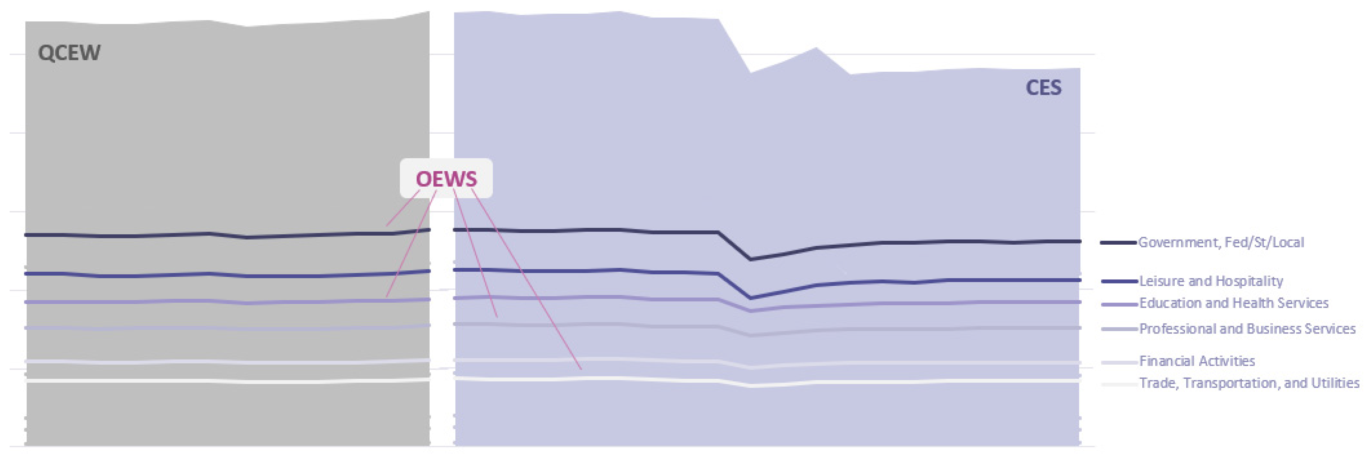
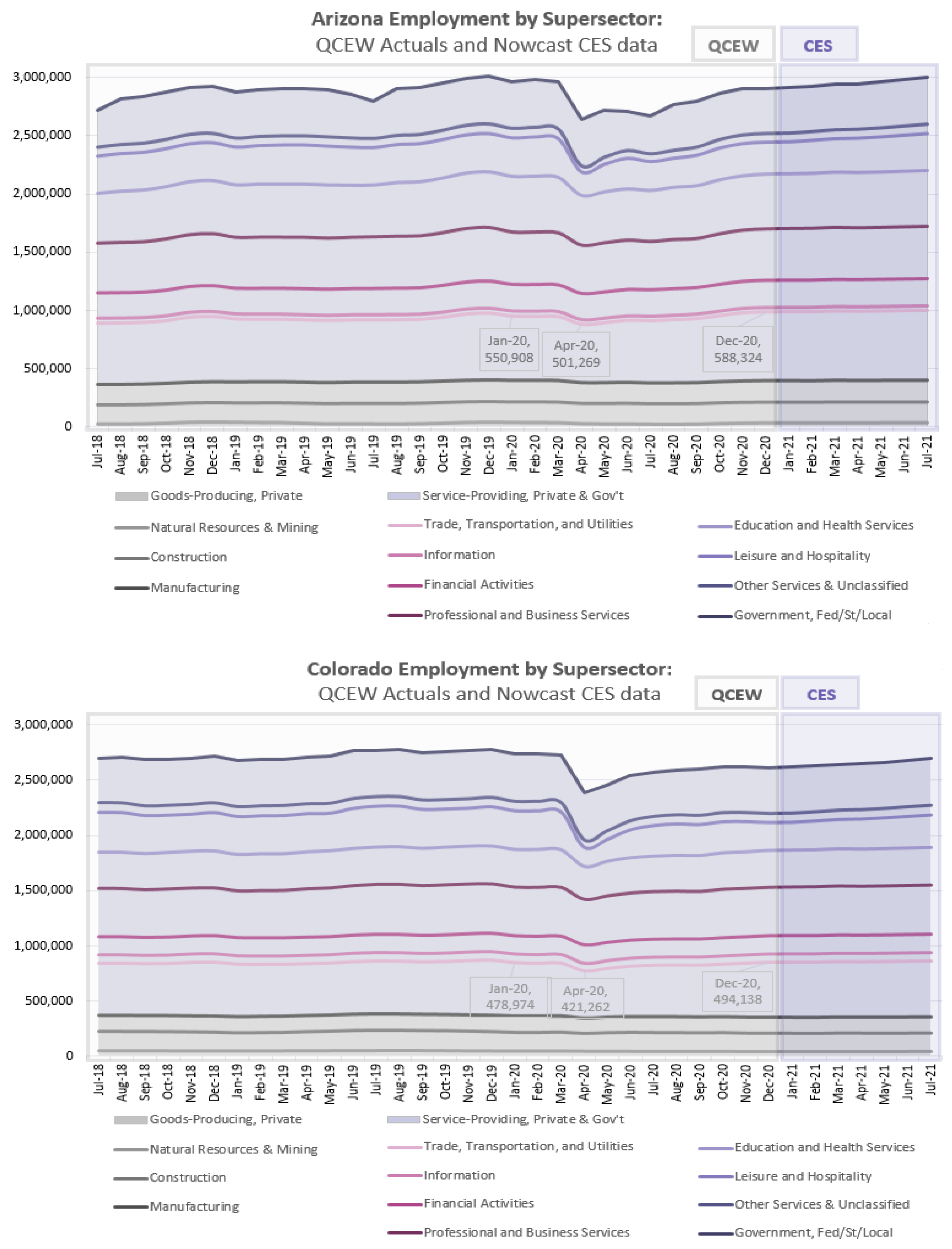
Having determined the value of a Multi-Level Nowcast for evaluating a variety of trends, the following section presents findings from using one to more closely examine key data. To recap at a high level, a Multi-Level Nowcast takes the most robust framework for the economy as a foundation (the QCEW, shown in grey in
Figure 4), updates it using the most current data available (the CES, shown in purple in
Figure 4), and then carves out areas of interest using income- or occupation-level data from the BLS’s Occupational Employment and Wage Statistics (OEWS, showing line-graph carveouts of key industry data in
Figure 4).
Common sense would suggest that COVID-19 has impacted the airline industry—but by precisely how much? How many workers, and of which skill levels, are being impacted by changes to air travel? What are the incomes of those experiencing employment changes, post COVID-19, and how does this differ between states? If a Multi-Level Nowcast is created, a researcher is suddenly able to address these questions, and many more. To illustrate, this paper compares and contrasts results for Arizona and Colorado, given their unique positioning and overall similar economies within the Mountain West Region. Testing impacts by job type requires using OEWS data to find the percentage of employment represented by the targeted group and then multiplying the Nowcast by these proportions. This creates a Multi-Level lens with which to evaluate current information.
3.1. Total Employment—Arizona vs. Colorado
The first step is to create a Nowcast for both economies so as to be able to directly compare shocks to the system in both locations. As previously described, this requires pulling QCEW data and updating them with the state’s portion of employment changes shown in the CES (
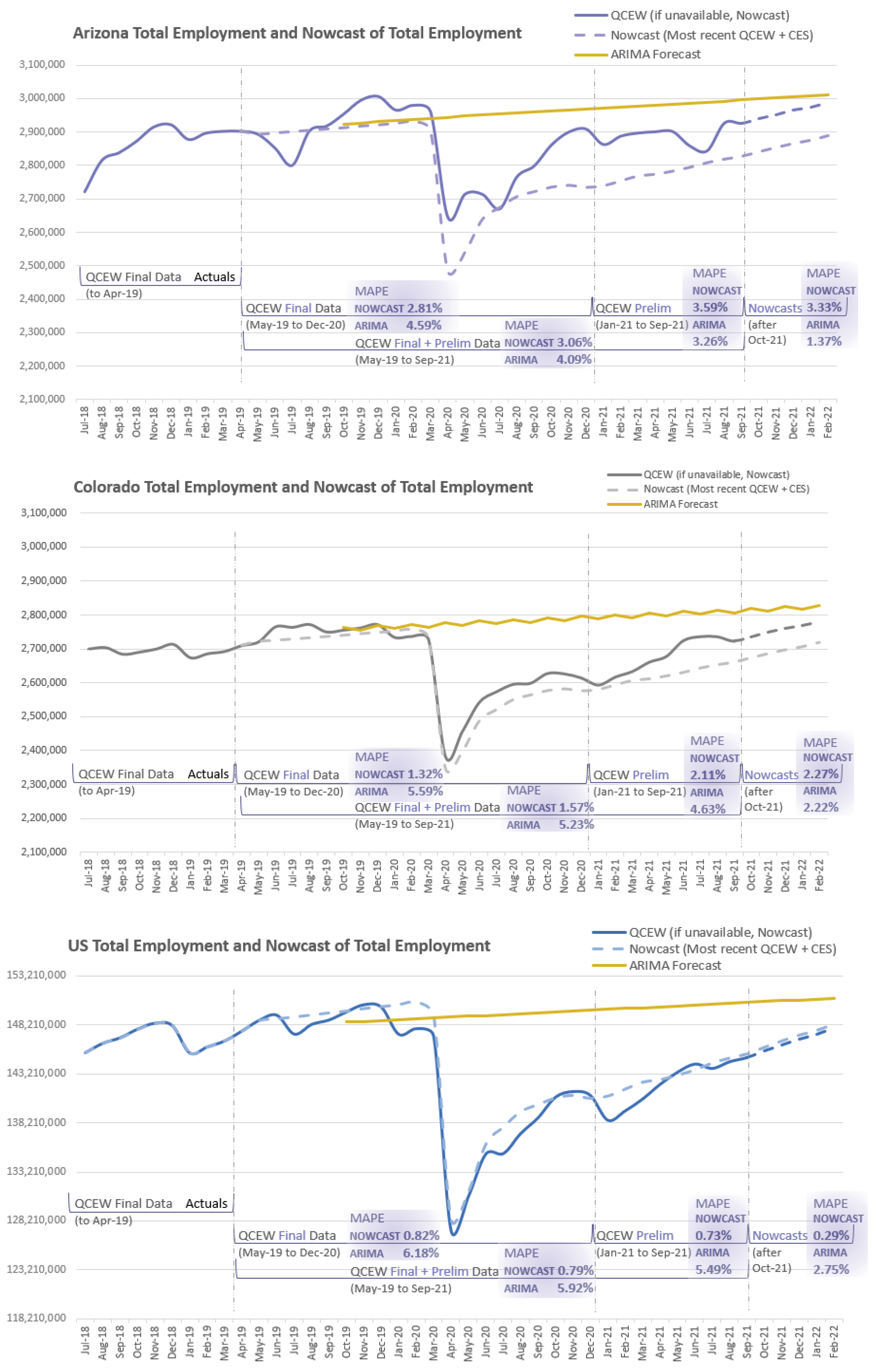
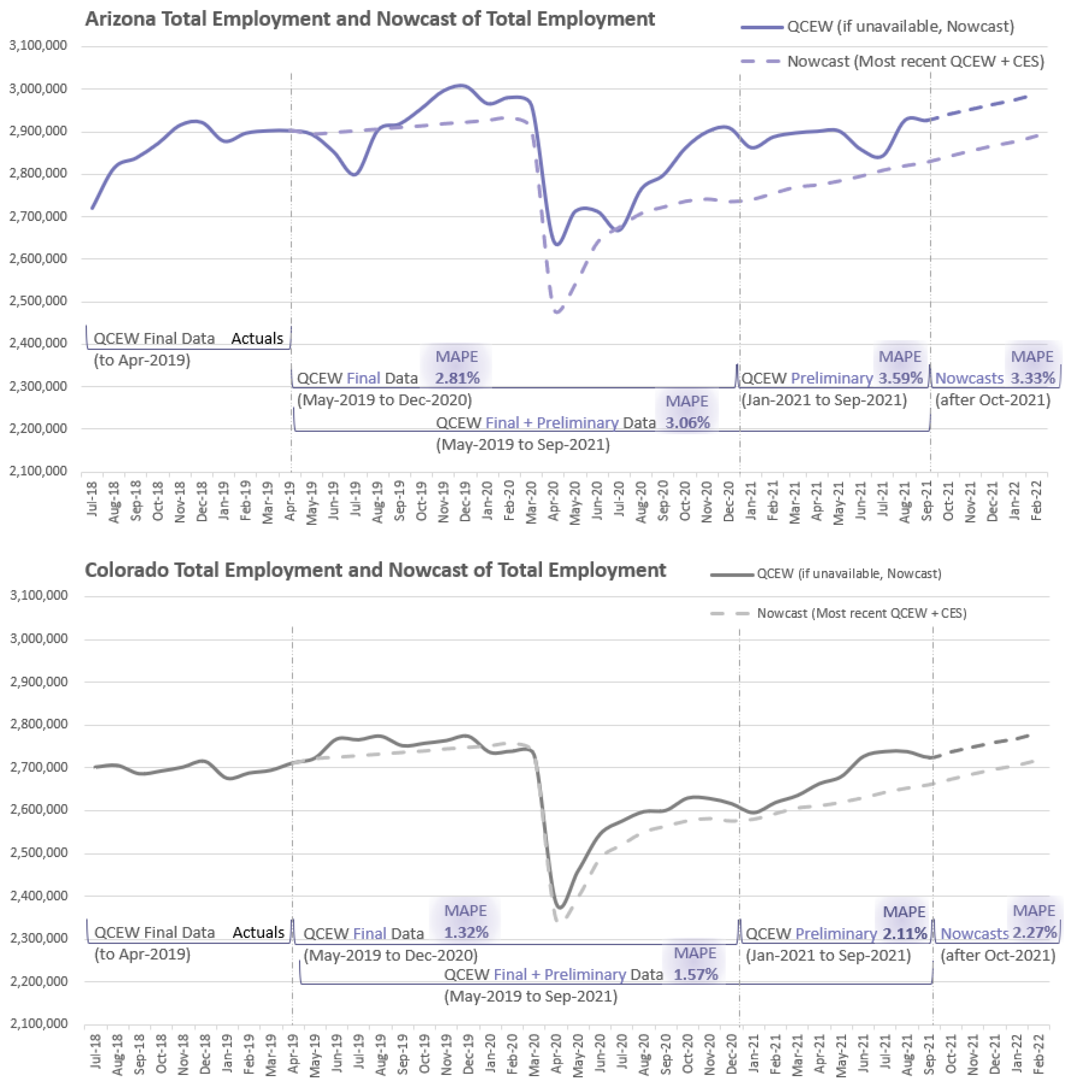
Figure 5). In both cases, actual QCEW data are presented as a solid line, while the Nowcast updates are reflected in the dashed lines. The darker line shows what is known today, given the most recent information available, while the lighter line captures what would have appeared by using the Nowcasting methodology on data that were available at the start of the COVID-19 pandemic and as the pandemic unfolded. In examining the descriptive statistics for each state, of key interest is the fact that the MAPE (Mean Absolute Percentage Error) is very consistent and quite low—well under 5% at the state level. This holds true in all cases—when comparing the Nowcast to Final QCEW data, to Preliminary QCEW data, to Final + Preliminary QCEW data, or when considering a Nowcast based on the QCEW data available when the pandemic hit (4/2019) vs. a Nowcast based on the most recent data as of this writing (preliminary QCEW of 9/2021). Of course, the final consideration of Nowcast to Nowcast has similar descriptive statistics due to CES data being a key part of each dataset, but the relationships and magnitudes remain similar to the evaluation of QCEW to the Nowcast portions of the dataset. These examinations were also performed for data for the US Total (50 States + Washington DC, excluding Puerto Rico, Guam, and the Virgin Islands), and all appeared to be of quite good quality, with a MAPE for all time periods of less than 1%. It is important to note that the data are holding up through some of the most difficult times that the US has ever experienced economically—it encompasses even the month of April 2020, when the economy shed more than 20 million jobs in a single month. Using quality data published by the QCEW and updating them with current-state CES numbers creates a strong Nowcast for immediate analysis and review of economic impacts.
We performed a simple test of potential systematic bias on both the Arizona and Colorado data by regressing the actual QCEW data on the Nowcast and a constant. The latter constants are insignificant, indicating there is no significant bias in the Nowcast. Furthermore, the regression coefficients are statistically indistinguishable from 1, indicating that the condition of a weak forecast rationality exists—further affirming the value of the Nowcast as a useful heuristic tool for practitioners.
These data show that Nowcasting remains a good approach. On a state-by-state basis, each proportional share of changes in the CES (+/−) as reflected in the Nowcast at times run counter to the standard US trend shown in
Figure 3. While the national trend shows QCEW employment data to be less than CES data, at times a state-level Nowcast, which uses CES data, can show values that are greater than QCEW due to a combination of CES data being run more quickly, details of CES methodology, and the way the Nowcast uses multipliers to estimate each state’s portion of changes to the CES. In all data examined for Colorado for this paper, this quirk does not present an issue, as all data points shown are within 4% of the eventual actual QCEW data, and inflection patterns are well-represented in the Nowcast information. In Arizona, 5 of the 15 data points are outside of the 4% ideal (Apr-20, 7.6%; May-20, 7.4%; Oct-20, 4.8%; Nov-20, 5.8%; and Dec-20, 6.2%), but again, inflection points, timing, and trend development all track the eventual QCEW data very closely. Looking at both state samples, if a researcher were presented with waiting months for quality QCEW data or being able to use the Nowcasted data immediately, having something instead of nothing would generally be preferable. Even a rough estimate would have given a much timelier sense of what was occurring and what recovery patterns were unfolding, long in advance of QCEW data being published.
3.2. Airline Employment—Arizona vs. Colorado
Given these two distinct regions, with differing histories and employment patterns, yet both undergoing the same crisis of a pandemic in the same sector of the economy—how have the shocks impacted each state on a supersector level? How many workers, and of which skill levels, are being impacted by changes to air travel? To evaluate, OEWS airline data are now overlaid on the Nowcast data in order to determine trends. All airline jobs under consideration in this evaluation occur within the Trade, Transportation, and Utilities supersector. For each year under consideration, airline employment as a percentage of the total supersector is calculated, and then multiplied against the Nowcast in order to have a current view of airline-specific data (
Figure 6). As with QCEW data, OEWS data are produced long after changes in the economy have occurred, barring researchers from evaluating updated information by using the standard dataset. By multiplying the Nowcast by OEWS trends, research can ostensibly be performed on industries of interest. In the absence of any other information, this methodology holds the employment pattern relationships constant in order to see what shocks to the supersector mean for the targeted subgroups. Common sense would suggest that COVID-19 has impacted the airline industry in Colorado—but by precisely how much?
The initial step in this effort is to split out the codes pertaining directly to airline workers to apply them to the OEWS dataset
1. Importantly, this paper does not attempt to evaluate ancillary impacts on employment, such as changes felt by restaurant workers employed at the airport or nearby hotel workers. Because federal bailouts to the largest 9 airline companies alone totaled over USD 35.78 billion, it seemed important to understand the scope and recovery patterns of this particular group (
Accountable.us 2021). The impacts of air travel on the economy undoubtedly ripple far beyond this limited scope of evaluation, but as a starting point, the airlines were of specific interest.
When evaluating the findings in
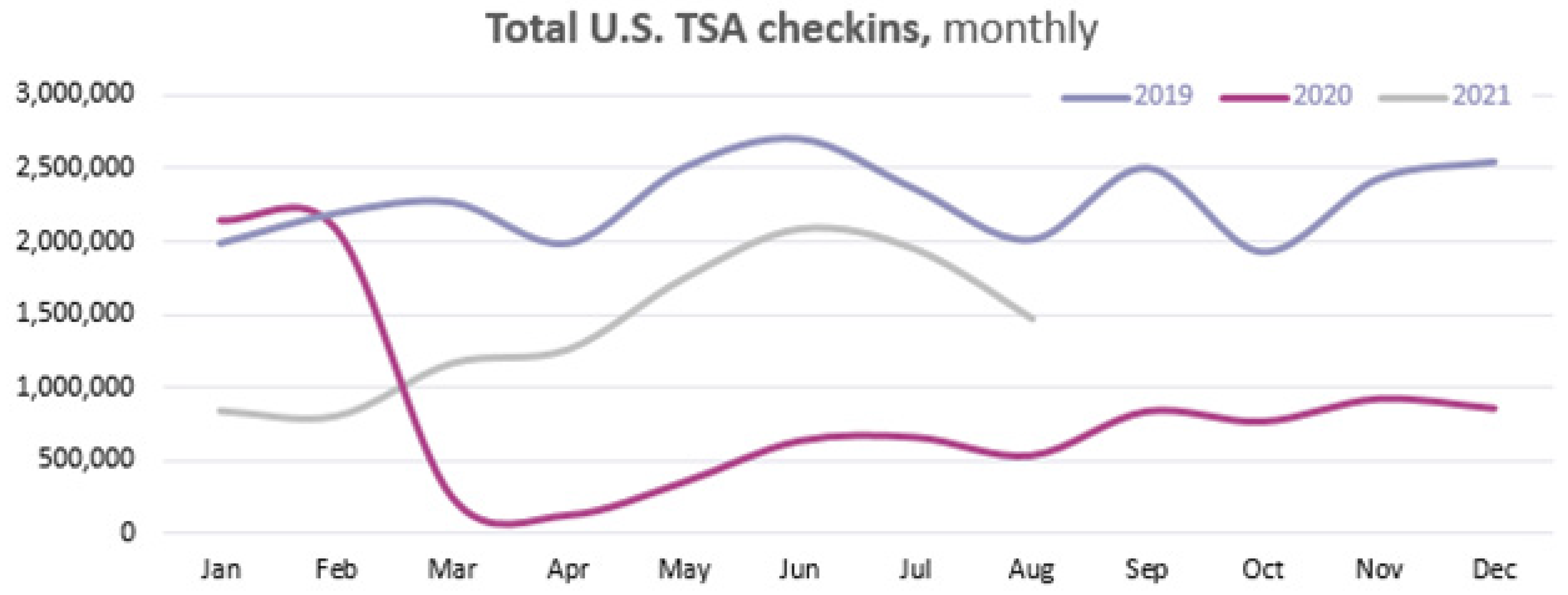
Figure 6, it appears that following the initial drop in airline employment in April of 2020, airline employment in both states has risen dramatically and not only recovered to a level above the peak travel season occurring before COVID-19 was present in the U.S.—in December 2019—it has risen by 3% in Arizona and 15% in Colorado. Yet TSA check-ins, which are a good proxy for airline traffic volumes, show that while the number of air passengers has recovered from the lows of 2020, air travelers are still far fewer than in 2019—Please see
Figure 7 (
Transportation Security Administration 2021). Anecdotal evidence suggests that ongoing struggles persist in airline operation, and no easy explanation comes to mind that addresses the 3–15% increase in airline employment shown in the Multi-Level Nowcast.
For guidance around this issue, let us backtrack and evaluate the Nowcast across all supersectors (
Figure 8). Looking at the underlying data, the issue becomes readily apparent. Because Airlines are in the supersector of Trade, Transportation, and Utilities, economic growth in areas, such as trucking and warehousing, are offsetting declines in air travel or other forms of trade. With the rise in online shopping, radical changes have been underway in how goods move through the economy, and future data will likely reflect this structural shift in the OEWS data. So, while the graphs in
Figure 6 are indeed representative of the proportion of the supersector’s employment as calculated using the 17 May–20 May OEWS datasets (3.5–4.8% of the Trade, Transportation, and Utilities supersector, depending on the state and year), there are not data yet on how the structural changes are impacting the overall makeup of state economies, employment within the supersector, or relationships among job categories within the one particular supersector. In this example, a
ceterus paribus assumption is
not a quality assumption due to the changing nature of work and consumer demand following the COVID-19 pandemic. This exercise surfaces how drastically people’s changing shopping habits are impacting state economies.
3.3. Impacts on Low-Wage Earners—Arizona vs. Colorado
Another interesting lens to consider is how changes in employment by supersector would impact lower-wage workers. Because the Nowcast is built on actual evolution within the economy by supersector (from the CES data), areas experiencing employment changes will be reflected in Nowcasted employment numbers. This is quite important since not all supersectors have been impacted equally by COVID-19, and wage distributions are not consistent among supersectors. Having insight into what this means for a state gives decisionmakers critical data for evaluating the economy. To be fair, the same issues presented applying the Multi-Level Nowcast to airline employment are still in play: if structural changes are occurring in the economy, applying percentages equally will mask specific evolutions. Researchers can compensate for this, however, by increasing or decreasing findings based on other areas of research. Examples would be adjusting for a K-shaped recovery, weighing frontline hospitality job losses more heavily, etc.
Having the OEWS data for each state in hand, it is easy to see that while the dataset can be evaluated by job title or supersector, it can also be evaluated by income level. For each occupation in the dataset, the total number of workers in the geography is given, and annual wages are presented at the 10%, 25%, 50% (median), 75%, 90%, and average (mean) salary levels. That is, if an occupation in a state has 1000 workers, and the 25% salary level for that occupation is USD 31,500, it can reasonably be inferred that those 250 workers in that role in the state make USD 31,500 or less. Further, it is possible to aggregate across all occupations in the state in order to understand what is occurring to workers at certain income levels in the economy. This reveals wide-ranging economic and policy implications.
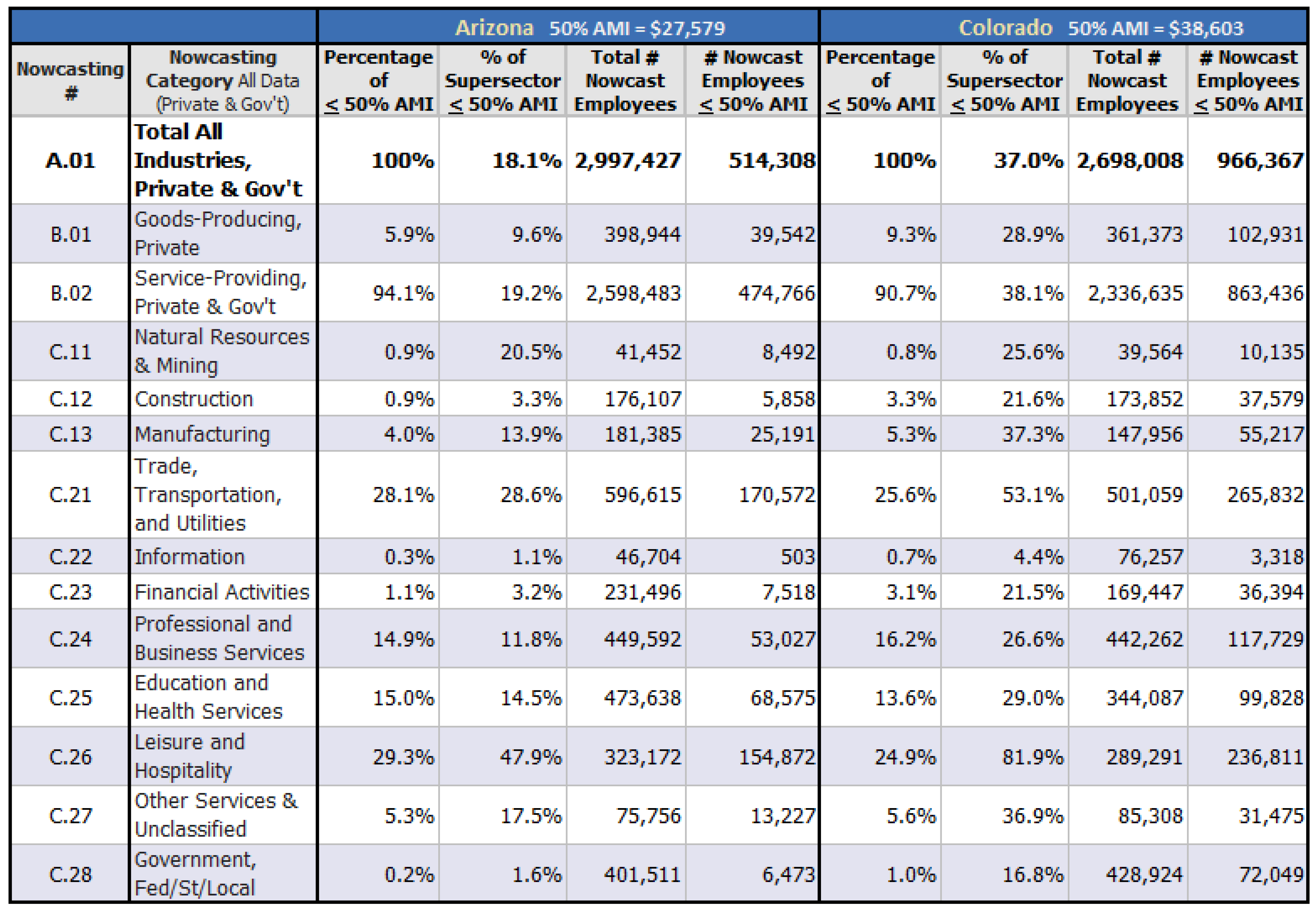
For this exercise, the Multi-Level Nowcast is evaluated not against airline workers for review, but rather against a weighted average of 50% Area Median Income (AMI) for all counties, to test how economic impacts appear using that measure. This measure is important because it shows the lower bound for many housing programs and is a good proxy for people who have some income, but who earn below half of what is common for the state. While AMI calculations do include data from many types of income, including those who are not in the workforce and collecting Social Security or other public benefits, it does provide an interesting lens with which to view a locale. After pulling population and income data for each county in the state and creating a statewide weighted average, 50% AMI is USD 27,579.05 in Arizona and USD 38,602.69 in Colorado. By interpolating between each known annual salary level by occupation code, the precise percentage of employment at 50% AMI can be calculated by supersector. That percentage is in turn multiplied by the number of workers in the Nowcast to estimate the current number of employees falling at or below 50% AMI.
Figure 9 illustrates the resulting values from these calculations.
From this calculation, it is easy to see several interesting themes:
Most workers earning under 50% AMI are in the Service-Providing sectors of the economy.
- ○
At 94.1% in Arizona and 90.7% in Colorado;
- ○
Specifically, the supersectors of Trade, Transportation, and Utilities as well as Leisure and Hospitality have very high percentages of low-wage workers;
- ○
This would make employees in these sectors especially vulnerable to lost work time or economic shocks, such as have been experienced under COVID-19.
While fewer employed people are low-income, at 18.1% of Arizona employees and 37.0% of Colorado employees, this finding illustrates how AMI data are skewed by citizens who are no longer in the workforce.
- ○
Within the evaluation of goods-producing supersectors, the Natural Resources and Mining sector stands out as having many low-wage workers, in large part due to agricultural wages;
- ○
Within Service-Providing portions of the workforce, again, the supersectors of Trade, Transportation, and Utilities (with retail employees) as well as Leisure and Hospitality (including hotel and restaurant workers) provide clear outliers as having many of their workers earning below 50% AMI.
Running the data, we find that in Arizona just over half a million workers earn below 50% AMI, while in Colorado, the number of low earners is close to one million employed workers.
- ○
Particularly with layoff and unemployment patterns that have arisen during the pandemic—with white collar workers being able to work remotely and having fewer layoffs due to changes in public health policies—it is clear that these low-earning workers are especially vulnerable.
These trends can help inform the dialogue between policymakers and economic experts.
- ○
Since not all parts of the economy are feeling the effects of the pandemic equally, having targeted data with which to inform decision making is particularly helpful.
As changes to these supersectors occur due to the COVID-19 pandemic—such as overall employment drops in Leisure and Hospitality or structural changes to Trade, Transportation, and Utilities due to altered shopping patterns—it is important to recognize that this will create real changes in state economies, the needs of their communities, and potential demand for social safety net offerings.
4. Conclusions: Importance of Multi-Level Nowcasting
This paper has discussed the methodology, application of, and findings derived by using a Multi-Level Nowcast to evaluate economic systems. As with any method of evaluation, there are strengths and weaknesses inherent to this approach, several of which have been presented transparently and indicate opportunities for future research efforts. However, amidst the dearth of information at the onset of the COVID-19 pandemic, it was always clear that state economies—with lockdowns occurring, viral transmission methods unclear, and industries in upheaval trying to remain profitable in a “new normal”—were experiencing a state of freefall, but no one knew quite how far economic conditions would fall or how far from the nadir conditions were. Particularly when considering trends that were impacting different sectors of the economy or different states unequally, it was very difficult to tell how deep or how badly the pandemic would affect our country. Being faced with momentous policy questions in this state of freefall—Subsidizing which industries will help the economy the most? What might future employment trends look like? Which citizens will need additional assistance, and for how long?—with limited to no data on which to run quality forecasts, with limited to no consensus between top institutions on how to approach looming questions, and with very little time to study or develop quality models … it was a feeling of helplessness unlike any other. Most of the time, a downturn occurs, researchers look to the past, attempt to adjust for current factors, and create a forecast. In the depths of this uncertainty, with no clear past data to evaluate, no clear way to adjust for current factors, and no solid guidance from thought leaders, Multi-Level Nowcasting as an insightful approach was created.
While this paper presents sample analyses of interest, there are many other places where further inquiry can occur. If Multi-Level Nowcasting is used more widely, the research approaches, valid areas of application, and general findings can be widely shared among various regions of the United States. There are so many ways that this analytical tool can assist in evaluating impacts on economies around the country that it is exciting to imagine prospective explorations. Finally, since the data can be run solely with manual extracts and manipulations, in a series of basic spreadsheets, this method is quite accessible to researchers of all types—creating a very wide range of possible future uses.
It is our sincere hope that by sharing this methodology, other researchers will recognize the value and applicability of this approach to other areas of interest. In time, this may yield new findings whereby positive impacts can be created through good decision making by informed actors. Without a current, quality estimation of the size and makeup of the economy in question, policymakers are not in a position to make the most educated, informed assessment, in light of current trends at play in the economy. Particularly in times of great upheaval, such as the COVID-19 pandemic, having updated, quality data is more valuable than ever. Multi-Level Nowcasting is an important tool for a variety of questions facing the American economy, particularly with the powerful updates created in the dataset, as well as with the highly targeted potential for additional investigations.
Author Contributions
Conceptualization, E.L.K.; methodology, E.L.K.; software, Not Applicable; validation, E.S., K.S. and S.W.; formal analysis, E.L.K. and S.W.; investigation, E.L.K. and K.S.; resources, E.S. and S.W.; data curation, E.L.K. and K.S.; writing—original draft preparation, E.L.K. and K.S.; writing—review and editing, E.L.K., E.S., K.S. and S.W.; visualization, E.L.K., K.S. and S.W.; supervision, E.L.K., E.S., K.S. and S.W.; project administration, E.L.K.; funding acquisition, Not Applicable. All authors have read and agreed to the published version of the manuscript.
Funding
This research received no external funding.
Institutional Review Board Statement
Not applicable.
Informed Consent Statement
Not applicable.
Data Availability Statement
Acknowledgments
The authors would like to acknowledge the valuable contribution of Gregory R. Miller at Department of Economics, CSU and external stakeholders at various stages of this endeavor.
Conflicts of Interest
The authors declare no conflict of interest.
Appendix A. A Brief Comparison of Nowcasting to ARIMA Model Approach Results
A careful reader may wonder how the Nowcasting methodology described in this paper compares in its predictive powers when considered with more conventional, even basic, approaches. To that end, we ran a quick ARIMA model using QCEW data from 2001 to September of 2019 for Colorado, then applied that model specification to Arizona and US Total QCEW datasets to see if the model’s predictive power produced better results than that of the Nowcast. This timeframe was used because it was the latest data that would have been readily available in March of 2020, when the COVID-19 pandemic began severely impacting the United States. The results were tested by running the standard accuracy criteria of RMSE, MAE/MAD, MSE, MAPE, and MPE. As the most readily comparable metric, the MAPE is presented for each segment of the dataset on the graphs directly for quick reference.
Comparing
Figure 5 with
Table A1 and
Figure A1, shown below, we can draw several conclusions, all of which bolster the argument for using a Nowcast when evaluating economic trends in uncertain times:
- 1.
The MAPE results are better for the Nowcast than for the ARIMA model.
Except for the three observations of AZ Prelim Only, AZ QCEW + CES, and CO QCEW + CES;
Particularly when considering the US Total results, these “better” results for AZ/CO would indicate that things are much worse for other states, balancing out the gains in these areas.
- 2.
The Nowcast results are a much better fit to the downturns occurring in the pandemic.
Because Nowcasting uses data from the QCEW and CES directly, any downturns are automatically incorporated into new data;
Which also eliminates adjustment variances that different researchers may choose to make when trying to account for economic changes in uncertain times;
Goodness of fit is not dependent on researcher expertise or luck.
Early on in the pandemic, there were many questions about economic recovery: when it might start, how it would impact different sectors of the economy, what form it would take, etc.
- 3.
Nowcasting can be performed as a “one-and-done” approach.
Essentially, the dynamic data being used in the Nowcast provide a much better approximation for actual future QCEW results than a simple ARIMA model, with less opportunity for error, less maintenance, and with fewer corrections required to keep the system up to date and ready to use. By not using past trends to define the equation describing expected employment, it yields a real-time representation of what is actually occurring in times of turmoil.
Table A1.
(
A–
C) Standard accuracy criteria for
Figure 5 and
Figure A1 comparing Nowcast to ARIMA model outputs.
Table A1.
(
A–
C) Standard accuracy criteria for
Figure 5 and
Figure A1 comparing Nowcast to ARIMA model outputs.
| (A) |
| Arizona Nowcast | RMSE | MAE/MAD | MSE | MAPE | MPE |
| Final Only | 96,370 | 79,757 | 9,287,178,866 | 2.81% | 2.239% |
| Prelim Only | 108,683 | 103,983 | 11,811,976,805 | 3.59% | 3.593% |
| Final + Prelim | 100,492 | 87,544 | 10,098,721,061 | 3.06% | 2.674% |
| QCEW + CES | 98,594 | 98,594 | 9,720,865,388 | 3.33% | 3.327% |
| Arizona ARIMA | RMSE | MAE/MAD | MSE | MAPE | MPE |
| Final Only | 158,252 | 126,768 | 25,043,701,975 | 4.59% | −3.378% |
| Prelim Only | 82,961 | 94,003 | 9,513,026,088 | 3.26% | −3.262% |
| Final + Prelim | 138,635 | 114,481 | 19,219,698,517 | 4.09% | −3.335% |
| QCEW + CES | 42,462 | 40,590 | 1,802,994,005 | 1.37% | −1.372% |
| (B) |
| Colorado Nowcast | RMSE | MAE/MAD | MSE | MAPE | MPE |
| Final Only | 38,075 | 34,533 | 1,449,701,227 | 1.32% | 1.171% |
| Prelim Only | 63,735 | 56,957 | 4,062,144,148 | 2.11% | 2.107% |
| Final + Prelim | 47,848 | 41,754 | 2,289,415,023 | 1.57% | 1.472% |
| QCEW + CES | 62,641 | 62,641 | 3,923,906,068 | 2.27% | 2.271% |
| Colorado ARIMA | RMSE | MAE/MAD | MSE | MAPE | MPE |
| Final Only | 183,407 | 141,904 | 33,638,277,110 | 5.59% | −5.532% |
| Prelim Only | 78,702 | 123,085 | 17,230,924,990 | 4.63% | −4.629% |
| Final + Prelim | 165,788 | 134,847 | 27,485,520,065 | 5.23% | −5.194% |
| QCEW + CES | 62,511 | 61,077 | 3,907,658,631 | 2.22% | −2.216% |
| (C) |
| US Total Nowcast | RMSE | MAE/MAD | MSE | MAPE | MPE |
| Final Only | 1,520,761 | 1,165,076 | 2,312,714,300,831 | 0.82% | −0.725% |
| Prelim Only | 1,327,070 | 1,032,842 | 1,761,114,891,140 | 0.73% | −0.610% |
| Final + Prelim | 1,461,306 | 1,122,572 | 2,135,414,490,573 | 0.79% | −0.688% |
| QCEW + CES | 422,354 | 422,354 | 178,382,901,316 | 0.29% | −0.288% |
| US Total ARIMA | RMSE | MAE/MAD | MSE | MAPE | MPE |
| Final Only | 10,677,790 | 8,366,965 | 114,015,200,638,241 | 6.18% | −5.822% |
| Prelim Only | 5,453,548 | 7,787,688 | 64,609,122,182,662 | 5.49% | −5.493% |
| Final + Prelim | 9,771,792 | 8,149,736 | 95,487,921,217,399 | 5.92% | −5.699% |
| QCEW + CES | 4,086,928 | 4,025,581 | 16,702,979,097,606 | 2.75% | −2.746% |
Figure A1.
State–level Nowcasts as compared to ARIMA model outputs.
Figure A1.
State–level Nowcasts as compared to ARIMA model outputs.
Appendix B. An Expanded Comparison—AR-X Benchmark Incompatibility with Nowcast
To be more specific in considering the Nowcasting methodology’s predictive power, we turn our attention to the possibility of using an AR-X model format, as recommended by one of our anonymous reviewers. In short, there are several reasons that AR-X is not a valid substitute for the Nowcasting approach detailed in this paper, with problems rooted in periodicity/calendar issues, non-stationarity, seasonality, structural breaks/fat tails, and model specification. Each of these issues is described in more detail below, hopefully providing full illumination around issues that would arise, were AR-X methods attempted to address the issues covered by Nowcasting.
Appendix B.1. Periodicity/Calendar Issues
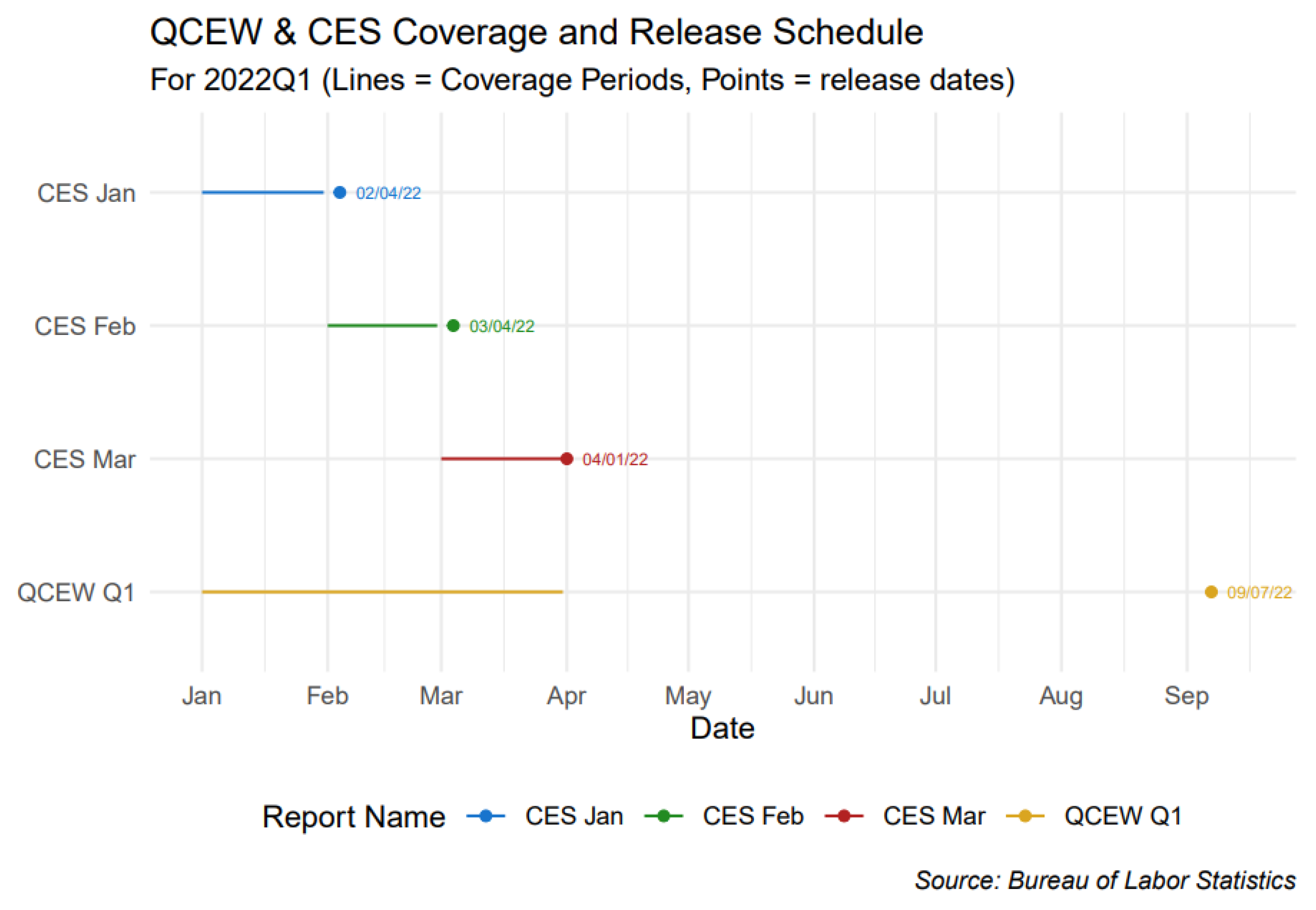
Among other things, the goal of the proposed Nowcast is to exploit the greater frequency of data collection of the Current Employment Statistics (CES) as compared to the Quarterly Census of Employment and Wages (QCEW) as well as to mitigate the substantial lag time between the end of the quarterly coverage period of the QCEW and the public release of the data. The frequency and lag time to release are illustrated below with reference to the as yet unreleased QCEW statistics for 2022Q1.
Figure A2.
Comparison of QCEW and CES release schedules.
Figure A2.
Comparison of QCEW and CES release schedules.
The Anonymous Referee (“Anon”) suggested that the Nowcast should be benchmarked against the predictive performance of an AR-X model. In particular, Anon suggested a model of the form
2: y
i,t+1 = c + αy
i,t + βx
i,t+1 + u
i,t+1, where y
i,t and x
i,t are the employment of industrial supersector i at time t according to the QCEW and CES, respectively.
Although it is not clear from Anon’s notation or comments which periodicity (quarterly or monthly) should be used, we will make the assumption that Anon meant monthly. Given the substantial lag time between the release of the full QCEW and for a given quarter and the component monthly CES releases, this means that even if potential end users of the AR-X model’s forecast were capable of running it themselves, they would need to contend with very wide confidence intervals on the forecast values. This is because they would need to forecast eight time steps ahead before the next QCEW release partially caught up with CES. These confidence intervals would also become even wider and mostly likely less accurate when they are most important (i.e., during times of heightened economic dynamism and uncertainty). Thoughtfully interpreting forecast results in such contexts requires exactly the type of audience expertise that our Nowcasting methodology aims to avoid.
While the AR-X model may be more robust or flexible for experienced users, it is not robust in terms of who can implement it. We address several more issues in this vein below.
Appendix B.2. Non-Stationarity
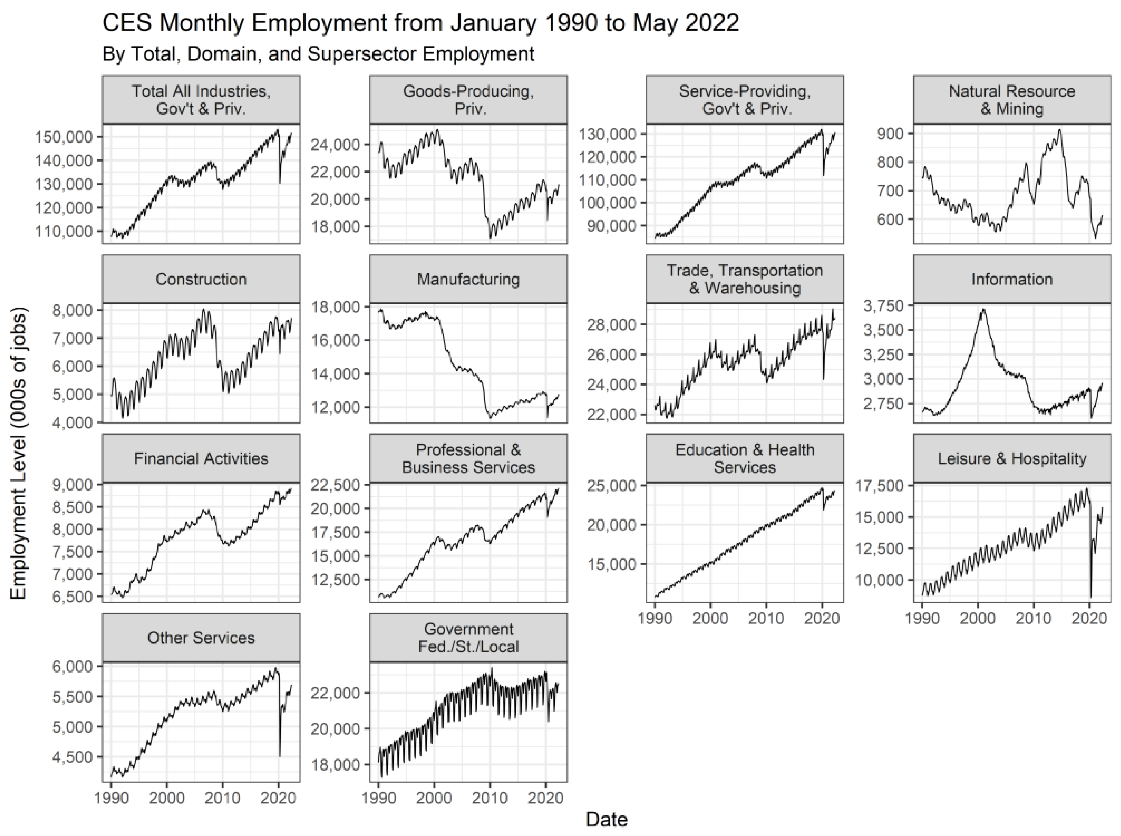
The figure below plots the evolution of total, domain, and supersector employment according to the CES for the entire time period for which there is both CES and QCEW data available. For this figure and the two that follow it, the patterns and features exhibited in the CES data are extant (although not precisely the same) in the QCEW data.
It is supremely obvious in the figure below that each time series is not stationary. Thus, in order to avoid completely spurious regression results, the end users of an AR-X model would need to first difference all the series (i.e., both the QCEW and CES for each industry).
Figure A3.
Evaluation of non-stationarity in CES monthly employment data (national) by supersector, January 1990—May 2022.
Figure A3.
Evaluation of non-stationarity in CES monthly employment data (national) by supersector, January 1990—May 2022.
Appendix B.3. Seasonality
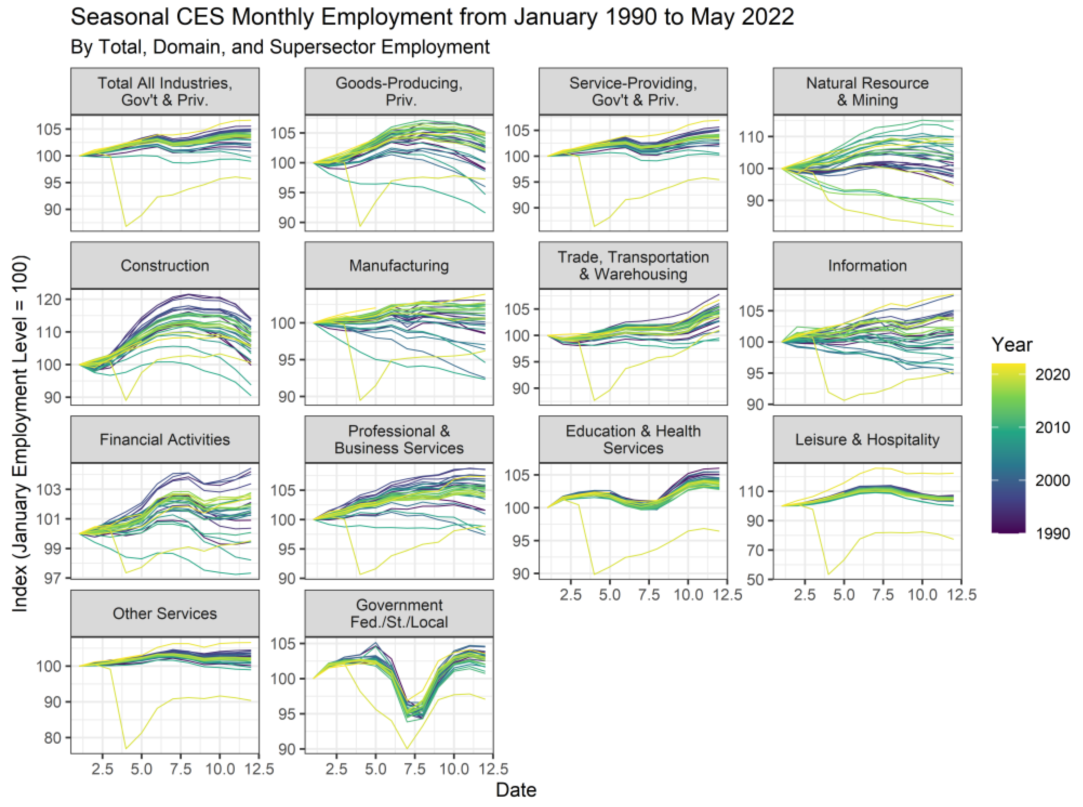
Seasonality is also a source of non-stationarity since the mean is not stable through the season. The figure below shows how employment changes over the course of each year in each time series by indexing two January employment levels as 100 and then updating over the next 11 months. Clearly, the majority of the time series exhibit very visible seasonality.
In order to mitigate this seasonality, the end users of an AR-X model would need to implement an appropriate method for de-seasoning the data. Seasonal differencing is the simplest but also the crudest method for achieving this objective. However, based on experience with smaller entities and local governments that do not employ dedicated economic professionals, this is still a somewhat onerous requirement for data preparation.
Figure A4.
Evaluation of seasonality in CES monthly employment data (national) by supersector, January 1990–May 2022.
Figure A4.
Evaluation of seasonality in CES monthly employment data (national) by supersector, January 1990–May 2022.
Appendix B.4. Structural Breaks/Fat Tails
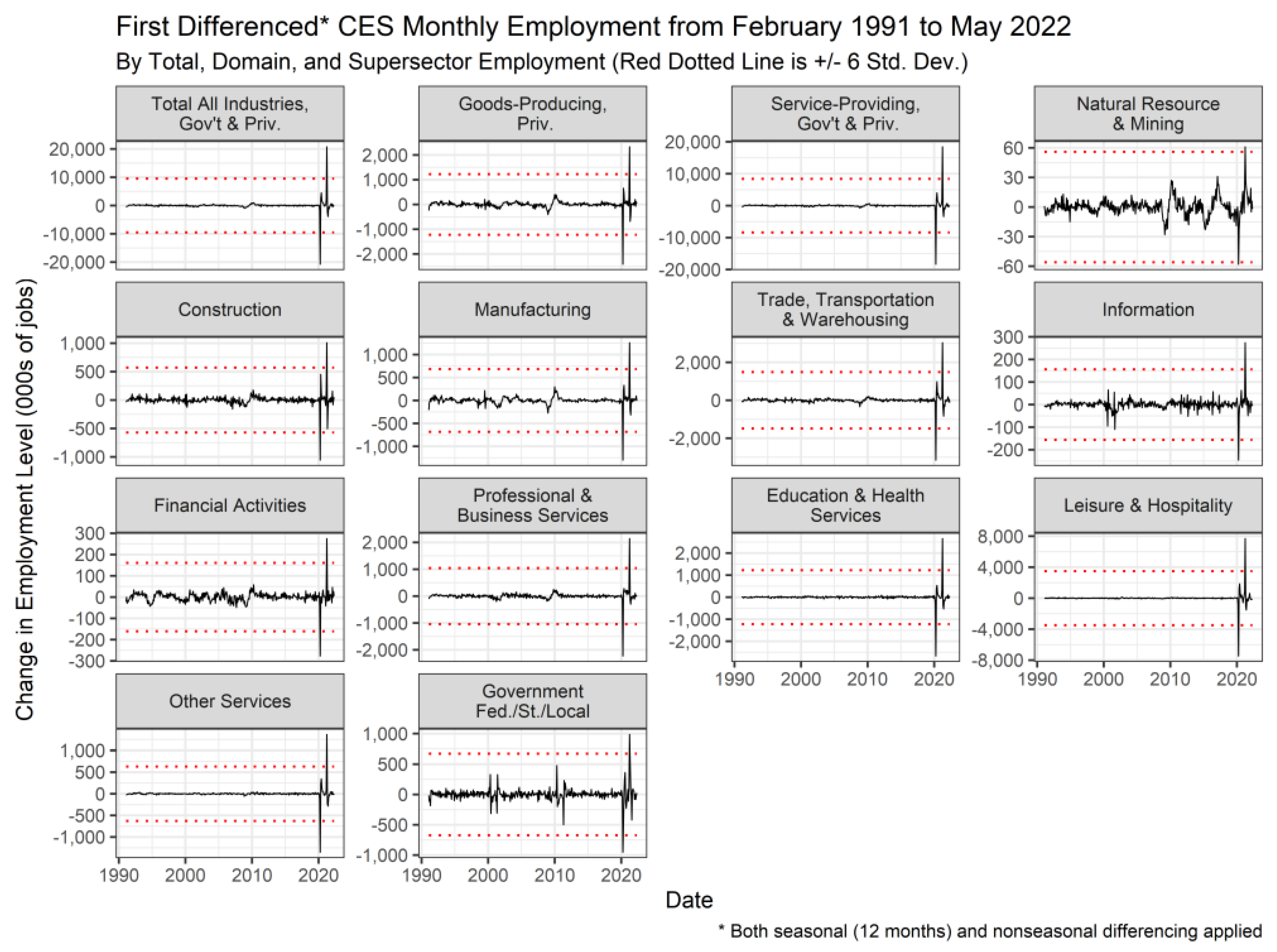
Supposing that the end users of our Nowcasting strategy could comfortably and reliably construct time series that were first differenced both seasonally and non-seasonally, there is still the issue that parametric modeling strategies, including the AR-X model, are not particularly robust to structural change. There are, of course, methods for identifying structural breaks, although depending on end users to implement these further reduces the number of entities that would have access to forecasts. Furthermore, it does not mitigate the issue of forecasting through a structural break in the data generation process or fat-tail event. To wit, the figure below shows the first differenced (seasonally and non-seasonally) time series in black with red dotted lines indicating +/− six standard deviations from the mean. Observations that are more than six standard deviations from the mean have one-in-half-a-billion chance of occurring. Every one of our time series witnessed observations at least this large, with some substantially larger.
Figure A5.
Evaluation of first differences of CES monthly employment data (national) by supersector, January 1990–May 2022.
Figure A5.
Evaluation of first differences of CES monthly employment data (national) by supersector, January 1990–May 2022.
Appendix B.5. Model Specification
Beyond the periodicity and calendar issues discussed above, which only set the baseline model specification needed to avoid predicting two time series simultaneously, there is the additional issue of lag structure/model identification that would optimize the performance of the AR-X model. Since we are considering 14 different time series, even if we could optimally identify the appropriate lag structure for each model within 4–6 attempts per model, then that would require us to run and evaluate between 112 to 168 individual AR-X models (2 states × 14 time series × 4–6 models per series). This is a very onerous request from Anon. However, in fairness to Anon, they suggested that we merely select models on the Bayesian Information Criterion (BIC). We are concerned though that this seems very much like data mining and would thus make us dubious about the appropriateness of the model selected for each time series as a benchmark.
If Anon is willing to more specific about the lag structure/model specification that they would prefer, then we are happy to run those particular models.
Appendix B.6. Conclusions
Resolution of all of the issues covered above may reasonably be expected to be part of the day-to-day responsibilities of an expert forecaster or time series econometrician. However, these professionals are not the target audience of our Nowcasting methodology. Any form of an AR-X model is not an appropriate benchmark since the fallback option for local governments and non-forecasting professionals is merely to wait for the release of data rather than attempt to find, learn to use, and then interpret the output of an AR-X model. Our methodology is not intended to be stringently rigorous, but rather to be relatively robust as well as simple and therefore easy to implement for governments and entities that cannot afford a staff economist. It is also intended to be less fragile with respect to fat-tail events than traditional time series models, which again require substantial skill to fortify and interpret in highly dynamic periods.
Appendix C. How to Build and Evaluate a Multi-Level Nowcast, Considering Specific Trends
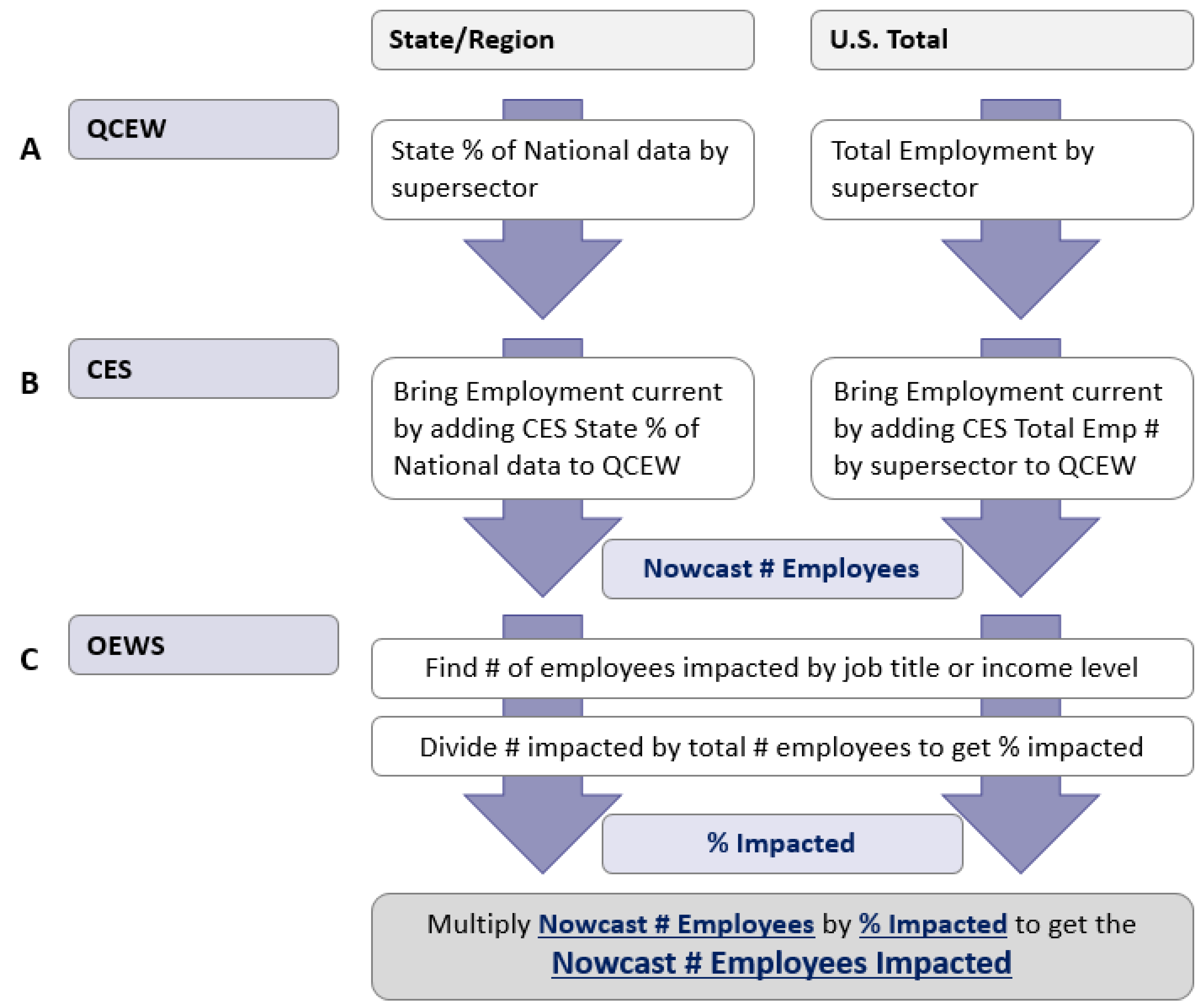
The value of creating a Multi-Level Nowcast has been detailed in this paper. This appendix describes the steps taken to build the dataset. This methodology allows other researchers to replicate, extend, and push analyses into areas not examined in this particular paper. To recap, a Multi-Level Nowcast takes QCEW data, updates it with CES data, then applies striations based on income- or occupation-level data from the OEWS. Breaking the steps down very simply, to create a Multi-Level Nowcast, the researcher must perform the following steps, as detailed in
Figure A6:
- 1.
Download data from the BLS: QCEW, CES, and OEWS.
- 2.
Create a key and apply it to the raw data.
This allows the different datasets to align and filters out any extra states.
It creates a standard, uniform crosswalk among all sources, particularly since each dataset is structured slightly differently.
The OEWS constantly shifts occupation codes—ensure all are represented before data use.
- 3.
Add CES data to QCEW data to obtain a current monthly employment value.
- 4.
OEWS employment data must be cleaned before they can be used.
- 5.
Find either the targeted jobs or the targeted income levels of interest, then apply the target percentage to OEWS data, quantifying the number of workers within the definition.
Figure A6.
Numbers and percentages of workers falling below 100% AMI and 50% AMI by supersector.
Figure A6.
Numbers and percentages of workers falling below 100% AMI and 50% AMI by supersector.
Step 1: Download data from the BLS. For every dataset, there are a number of ways to access the data. Rather than prescribe a specific route, this paper describes the final data needed—the researcher can then determine the easiest way for them to access that particular dataset.
| QCEW data require | Monthly data, seasonally adjusted; |
| | Private and federal/state/local government employment; |
| | At a state/national level; |
| | Total all industries (10), Domains (101, 102), and Supersectors (1011 … 1029). |
| CES data must have | Employment changes by industry; |
| | As shown in the CES Publication of Employment and Earnings “Summary Table B…”; |
| | (“Summary Table B. Establishment data, seasonally adjusted”). |
| OEWS data need | Annual data by job with employment and 10/25/50/75/90 percentile wages; |
| | On a state and national level; |
| | All levels: Detailed occupation codes > Major industry codes > Total for the state. |
Step 2: Create and apply keys to raw data. In order to have every dataset align to the other, the researcher must create a series of keys or crosswalks to have all pieces come together successfully.
| Key A—State/Region | Create a key that filters the data by state/region of interest; |
| | Omit unwanted locations (e.g., Puerto Rico, Guam, Virgin Islands, etc.); |
| | For the OEWS, Total U.S. data are often too aggregated—the dataset is more precise if all state data are summed into a “U.S. Total”. |
| Key B—QCEW | Create a key that separates and sums Totals, Domains, and Supersectors nicely at a state or national level; |
| | Make sure that Government and Unclassified data are represented as desired. |
| Key C—CES | Create a key that maps employment categories into the QCEW Key structure; |
| | Aligning the CES with the basic QCEW definitions; |
| | At times, this requires extra summations in order to line up the categories. |
| Key D—OEWS | Create a key that puts occupational codes into a corresponding industry; |
| | The role is in several industries, but overall market is driven by one major group. |
| Key E—Target Jobs | If analyzing a group of jobs (e.g., airline workers), create a key for relevant roles. |
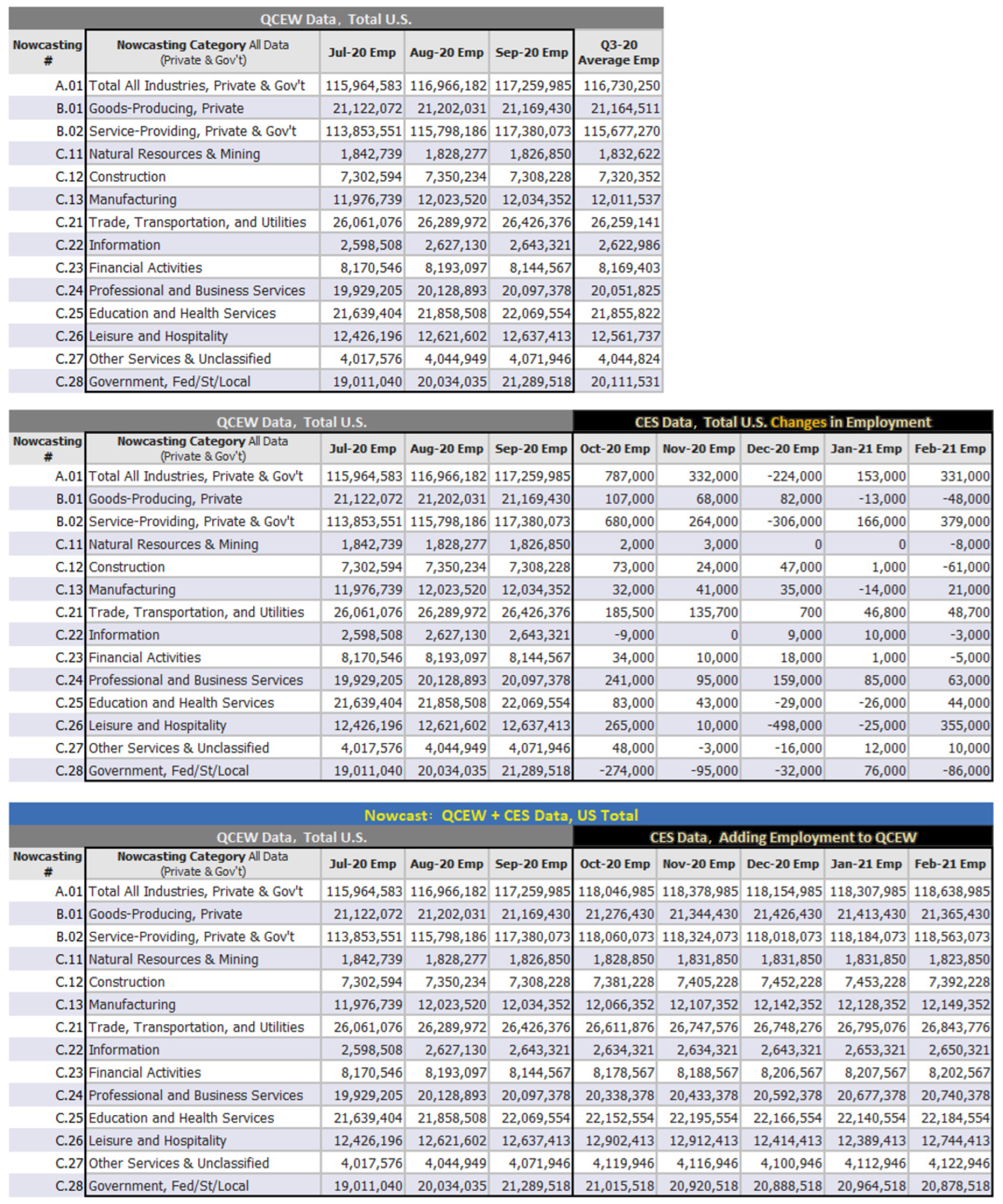
Step 3: Add CES data to QCEW data to obtain a current monthly employment value. Using the processed data that have been run through the keys, add the CES data to the QCEW data. Remember that the CES data need to be translated to proper units; for instance, national employment changes shown in the CES’s “Summary Table B…” has the unit of thousands, while the QCEW presents employment in single units. The CES also usually shows changes to overall employment, so the months must be continuous for the data to be accurate. At a national level, the datasets can simply be added together—see
Figure A7 for details.
Figure A7.
Progression of creating a Nowcast for Total U.S. data.
Figure A7.
Progression of creating a Nowcast for Total U.S. data.
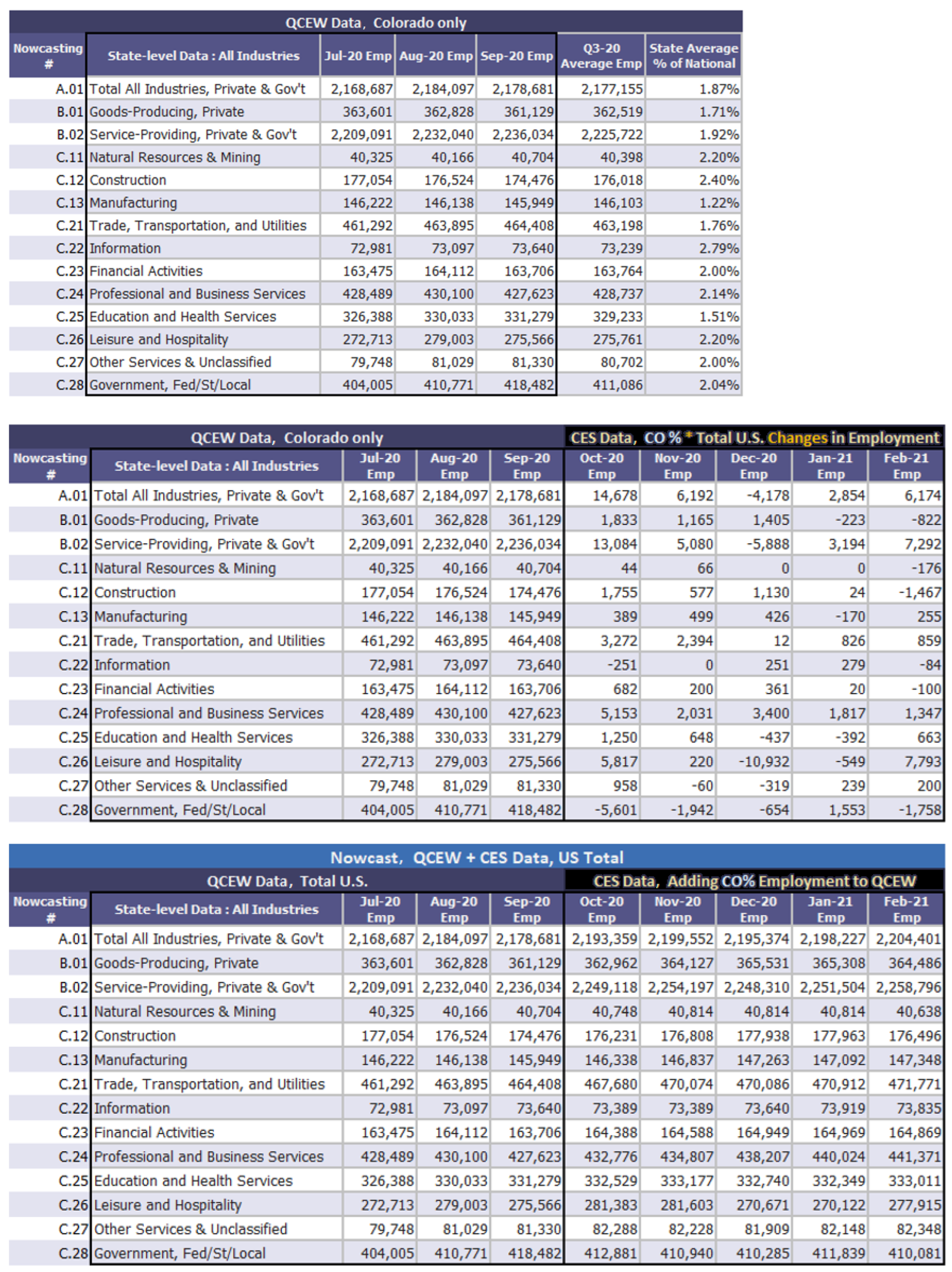
At a state or regional level, this simplified approach will not work because CES is only shown nationally and does not align to a single state/region. The fix is simple: Find the most recent quarter’s percentage of employment by supersector for state/region in the QCEW. Then multiply that percentage to the CES data in order to add the correct portion of the national employment to the state/region of interest. This does assume that the proportional changes by state/region stay constant from the most recent QCEW to the current CES, which admittedly is not perfect, since some regions are bound to be hit harder than others. However, in the absence of other information, this is the best way to understand changes in the nation’s labor markets, updated to current times. See
Figure A8 for details.
Figure A8.
Progression of creating a Nowcast for Colorado state data.
Figure A8.
Progression of creating a Nowcast for Colorado state data.
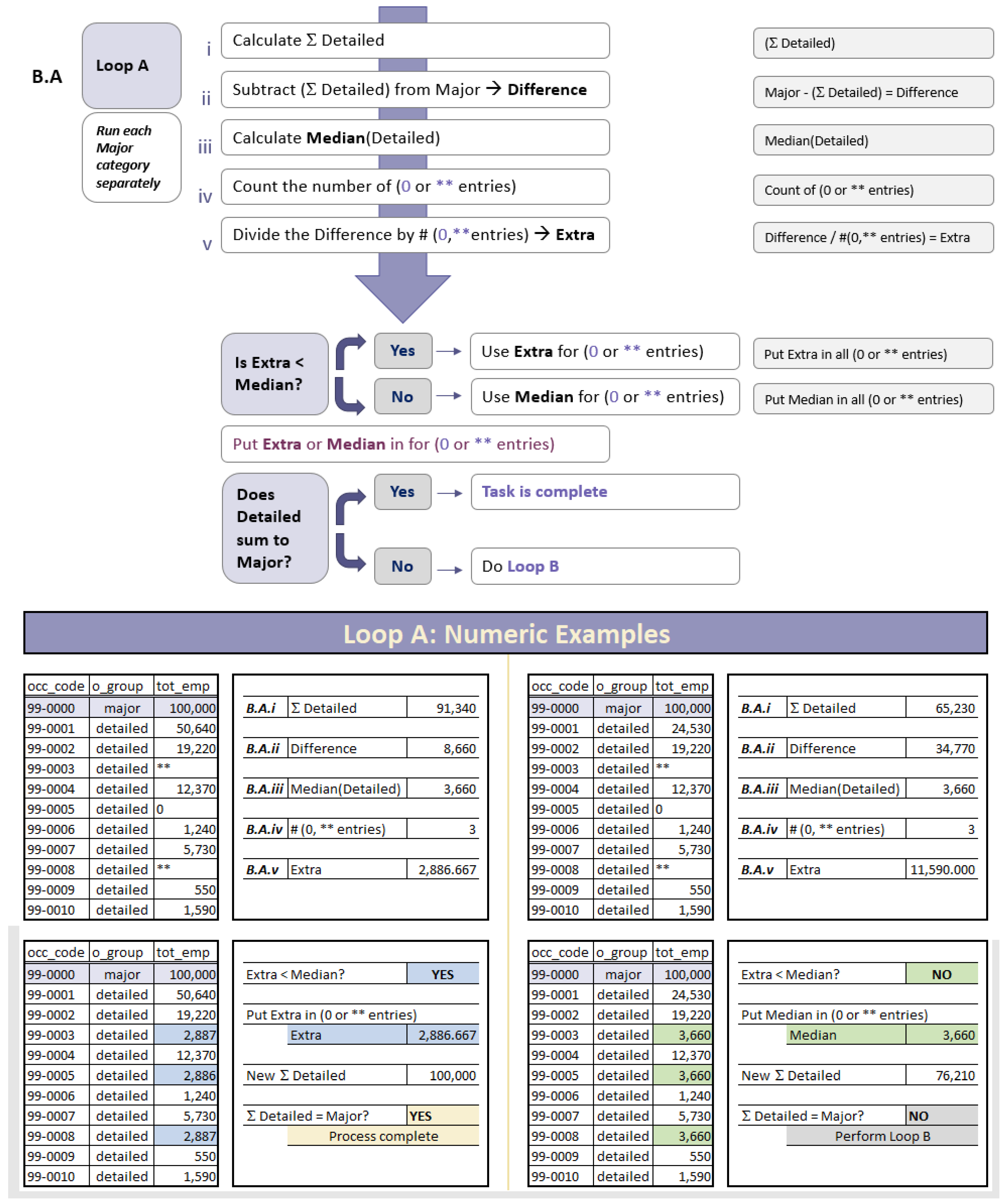
Step 4: OEWS employment data must be cleaned before they can be used. In theory, for any given state, employment would sum from Detailed (occ_code = xx-yyyy) up to Major (industry codes; xx-0000 of the occ_code data) and Major up to Total (00-0000). Unfortunately, for a variety of reasons, this is not the case. Luckily the fix is easy: by industry code group for the state, fill in any entries that have 0 or ** with quality approximations, then distribute any excess employment proportionally to the detailed occupations. See
Appendix D for details and methodology used in this paper.
Step 5: Find either the targeted jobs or the targeted income levels of interest, then apply the target percentage to OEWS data, quantifying the number of workers within the definition. While it is nice to have updated overall employment data, as found in Step 3, it is even better to be able to understand the impacts of economic developments or various policies on different populations. First, define the population of interest—either by occupation code (occ_code) or income level (as applied to a_pct10, a_pct25, a_mean [50%], a_pct75, a_pct90)—to be able to carve out the information for this group. After clearly defining the group of interest, a researcher now has concrete information that is based on actual employment and wage data. Calculate the percentage that meets the targeted criteria, then multiply it by the updated employment data found in the Nowcast to obtain a final, Multi-Level Nowcast, focused on the areas of interest. This approach is illustrated in detail in
Section 3 of this paper.
Importantly, for the U.S. as a whole, it is safest to run the data for all states and then aggregate up to the country’s total. Particularly when working with the annual incomes presented (the a_pctX mentioned previously), the spans between different income levels are too broad on a national level to be widely useful. States also have uneven distributions of high and low wages, and highly heterogeneous wage floors, given state-level minimum wage regulations. Aggregating all state information to a national total allows for a very detailed breakdown of the information. And since employment patterns have changed due to the data only being published annually, it also allows for the evolution of the economy in the present tense. Particularly in times of great upheaval—such as the COVID-19 pandemic—these updated, detailed data are very valuable from a research standpoint.
Appendix D. Process to Ensure OEWS Data Totals from “Detailed → Major → Total”
![Economies 10 00194 i001]()
![Economies 10 00194 i002]()
![Economies 10 00194 i003]()
Notes
| 1 | Codes used include (occ_code/occ_title)—53-2021/Air Traffic Controllers, 53-1041/Aircraft Cargo Handling Supervisors, 49-3011/Aircraft Mechanics and Service Technicians, 53-6098/Aircraft Service Attendants and Transportation Workers, All Other, 53-2022/Airfield Operations Specialists, 53-2011/Airline Pilots, Copilots, and Flight Engineers, 43-5011/Cargo and Freight Agents, and 53-2031/Flight Attendants. In many states, 43-5011/Cargo and Freight Agents are primarily non-airline in nature, but in Colorado most are employed by airlines and thus are included in the analysis. |
| 2 | Anon actually suggested a model of the form yi,t+1 = c + αyi,t + βixt+1 + ui,t+1. The authors assume this was a typing error since we have and utilize supersector employment in both QCEW and CES data. |
References
- Accountable.us. 2021. COVID Bailout Tracker. Available online: https://covidbailouttracker.com/program/airline-industry-bailouts (accessed on 3 March 2021).
- Bartik, Alexander W., Marianne Bertrand, Feng Lin, Jesse Rothstein, and Matt Unrath. 2020. Labor Market Impacts of COVID-19 on Hourly Workers in Small- and Medium-Sized Businesses: Four Facts from Homebase Data. University of Chicago, Booth School of Business; Rustandy Center for Social Sector Innovation, April. Available online: https://irle.berkeley.edu/labor-market-impacts-of-covid-19-on-hourly-workers-in-small-and-medium-sized-businesses-four-facts-from-homebase-data-2/ (accessed on 15 February 2021).
- Button, Kenneth, and Somik Lall. 1999. The Economics of Being an Airport Hub City. Research in Transportation Economics 5: 75–105. Available online: https://www.sciencedirect.com/science/article/abs/pii/S0739885999800055 (accessed on 3 March 2021). [CrossRef]
- Goolsbee, Austan, and Chad Syverson. 2020. Fear, Lockdown, and Diversion: Comparing Drivers of Pandemic Economic Decline 2020. In National Bureau of Economic Research. NBER Working Paper No. 27432. June, Available online: https://www.nber.org/papers/w27432 (accessed on 13 February 2021).
- International Civil Aviation Organization. 2021. Effects of Novel Coronavirus (COVID_19) on Civil Aviation: Economic Impact Analysis. Economic Development—Air Transport Bureau. Available online: https://www.icao.int/sustainability/Documents/COVID-19/ICAO_Coronavirus_Econ_Impact.pdf (accessed on 20 February 2021).
- Kaiser Family Foundation. 2020. Eligibility for ACA Health Coverage Following a Job Loss. May. Available online: https://www.kff.org/report-section/eligibility-for-aca-health-coverage-following-job-loss-methods/ (accessed on 20 June 2020).
- Leibovici, Fernando, Ana Maria Santacreu, and Matthew Famiglietti. 2020. Social Distancing and Contact-Intensive Occupations. St. Louis: Federal Reserve Bank of St. Louis, March, Available online: https://www.stlouisfed.org/on-the-economy/2020/march/social-distancing-contact-intensive-occupations (accessed on 15 February 2021).
- Lewis, Daniel J., Karel Mertens, and James H. Stock. 2020. Monitoring Real Activity in Real Time: The Weekly Economic Index. Liberty Street Economics 20200330b. New York: Federal Reserve Bank of New York. [Google Scholar]
- McGraw, Marquise J. 2016. Does Airport Size Matter? Hub Airports and Local Economic Questions. OpenTable 2020. State of the Industry. Available online: https://www.opentable.com/state-of-industry (accessed on 3 March 2021).
- Parolin, Zachary, and Christopher Wimer. 2020. Forecasting Estimates of Poverty during the COVID-19 Crisis. Poverty and Social Policy Brief, 2046. New York: Center on Poverty and Social Poverty, Columbia University. [Google Scholar]
- Petrosky-Nadeau, Nicolas, and Robert G. Valletta. 2020. Unemployment Paths in a Pandemic Economy. Federal Reserve Bank of San Francisco Working Paper 2020-18. Available online: https://www.frbsf.org/economic-research/files/wp2020-18.pdf (accessed on 20 February 2021).
- STR. 2020. COVID-19: Hotel Industry Impact and Recovery. Available online: https://str.com/data-insights-blog/coronavirus-hotel-industry-data-news (accessed on 20 February 2021).
- Transportation Security Administration. 2021. TSA Checkpoint Travel Numbers. Available online: https://www.tsa.gov/coronavirus/passenger-throughput (accessed on 20 February 2021).
- U.S. Bureau of Labor Statistics. 2021. All Employees, Air Transportation [CES4348100001]; Retrieved from FRED. St. Louis: Federal Reserve Bank of St. Louis. Available online: https://fred.stlouisfed.org/series/CES4348100001 (accessed on 30 April 2021).
| Publisher’s Note: MDPI stays neutral with regard to jurisdictional claims in published maps and institutional affiliations. |
© 2022 by the authors. Licensee MDPI, Basel, Switzerland. This article is an open access article distributed under the terms and conditions of the Creative Commons Attribution (CC BY) license (https://creativecommons.org/licenses/by/4.0/).
