Article

Regional Wage Differences and Agglomeration Externalities: Micro Evidence from Thai Manufacturing Workers

by
Nutchapon Prasertsoong
and
Nattapong Puttanapong
*
Faculty of Economics, Thammasat University, Bangkok 10200, Thailand
*
Author to whom correspondence should be addressed.
Economies 2022, 10(12), 319; https://doi.org/10.3390/economies10120319
Submission received: 1 November 2022 / Revised: 5 December 2022 / Accepted: 7 December 2022 / Published: 12 December 2022

Abstract

:
The large and persistent wage gap between the Bangkok Metropolitan Region and its peripheries remains a major concern for policymakers and civil society. Theoretically, these regional disparities exist due to differences in workforce skills and the local characteristics of the regions. This study empirically investigates the sources of spatial wage disparity in Thailand using data sets from the Labor Force Survey, the Industrial Census, geospatial data, and satellite imagery for the years 2007, 2012, and 2017. The two-stage estimation method was applied, and the soil clay content was used as the instrumental variable for correcting endogeneity and variable bias omission. The results show that workers’ education and experience affect the wage differential. Other than individual skills, workers also benefited from the agglomeration externalities of large cities. Specifically, the effect of agglomeration externalities on wages in Thailand was found to be statistically significant. To overcome the paradox of a low urbanization rate and high urban primacy in Thailand, this study suggests the establishment of multiple regional cities that create high agglomeration externalities.

1. Introduction

The structural transformation of the Thai economy has continuously progressed since the implementation of the first national development plan in 1961. Concentrated economic activities have evolved from agriculture to industrial production and services. This development process has also expanded the urbanized areas. Currently, however, economic activity and the population are concentrated in Bangkok and the adjacent vicinities, formulating a monocentric growth pattern. In particular, Thailand’s high magnitude of urban primacy, ranked among the highest in the world, has been repeatedly documented (Dixon 1999; Richter 2006; Short and Pinet-Peralta 2009; Limpanonda 2012; Puttanapong 2018).
Thailand has simultaneously experienced declining GDP growth and spatial inequality for two decades. Due to the persistent spatial disparity of income and the steep rank-size distribution of the cities, quantifying the contribution of agglomeration externalities is essential for future regional development plans. However, as stated by Duranton (2014) and Chauvin et al. (2017), the evidence from developing countries is very limited, including that detailing the Thai experience. Hence, this study identifies the source of regional wage differences in Thailand. A two-stage estimation method was applied to distinguish the effects of labor productivity from regional characteristics (Combes et al. 2008; Groot et al. 2014; Ridhwan 2021).
The remainder of the study is organized as follows: Section 2 outlines the related literature, focusing on both theoretical and empirical studies; Section 3 then provides an overview of the data used in this analysis; Section 4 presents details on the research methodology; Section 5 discusses the obtained results and their policy implications; and Section 6 concludes with the main contributions and suggestions for future research.

2. Literature Review

2.1. Theoretical Studies

As comprehensively reviewed by Combes and Gobillon (2015), the theoretical foundations of agglomeration were established by Marshall ([1920] 1890), suggesting that larger cities gain higher economies of scale. Agglomeration exponentially benefits big cities through knowledge spillovers, labor market pooling, and backward–forward intermediate input linkages. Glaeser et al. (1992) integrated the key concepts formerly introduced by Marshall ([1920] 1890); Arrow (1962); and Romer (1986) to characterize the Marshall–Arrow–Romer (MAR) spillover, which is the knowledge spillovers that occur within geographical and industry-specific concentrations. Meanwhile, Jacobs (1969) documented evidence of cross-sectoral knowledge spillovers, subsequently titled the Jacobs spillover. Porter (1990) suggested that cities foster knowledge spillovers through highly competitive markets and geographically specialized industries (later recognized as the Porter spillover).
Alternatively, Fujita et al. (1999) and Krugman (1999) pioneered the new economic geography theory, mathematically modeling the agglomeration force and spatial distribution of economic activities. In particular, this modeling approach incorporates imperfect competition and the distance decay transportation cost, allowing the quantitative framework to examine relationships among increasing return to scale, location, and agglomeration.
Duranton and Puga (2004) proposed the most recent and widely referred to theoretical framework, which considers agglomeration economies as a combination of sharing, matching, and learning. Specifically, the sharing effect stems from a density of industrial specialization and a variety of inputs coupled with a greater opportunity to access public goods and risk pooling. Meanwhile, the matching effect is the consequence of a thick labor market which subsequently improves the matching efficiency of job applicants and firms. Lastly, the learning effect mainly functions through the knowledge spillover mechanism.

2.2. Empirical Studies

Following the fundamentals proposed by Marshall ([1920] 1890), Kelley (1977) introduced the quantitative technique for investigating empirical evidence of city agglomeration and consequently guided the analytical framework for various subsequent studies, including the studies of Sveikauskas (1975); Nakamura (1985); Henderson (1986); Moomaw (1998); and Henderson (2003).
Moomaw (1981) is among the earlier scholars proposing critiques on estimating agglomeration elasticity. Improvements to the empirical strategy are continuously undertaken later on. As extensively surveyed by Combes and Gobillon (2015), the main aspects of development are the econometrical methods and endogeneity concerns (see detailed discussion in Combes et al. (2011) and Baum-Snow and Ferreira (2015)). To combat the endogeneity problem, Ciccone and Hall (1996) and Combes et al. (2008) introduced the two-stage least squares estimation, which subsequently became the conventional method in the discipline.
Rosenthal and Strange (2004); Beaudry and Schiffauerova (2009); de Groot et al. (2009); Melo et al. (2009); and Puga (2010) systematically reviewed the related literature. These surveyed empirical studies commonly show that if the city population or density doubles, productivity (measured by wages or total factor productivity) increases by 1–10%. Alternatively, Grover et al. (2021) applied the meta-analysis method to the estimated coefficients of 70 studies in 33 countries. The obtained results showed that doubling the city size is associated with a 4–6% increase in productivity for developing economies. However, the difference in agglomeration elasticity between developed and developing countries remains econometrically inconclusive.
For Thailand, Southichack (1998) and Limpanonda (2012) applied Ciccone and Hall’s (1996) method to Labor Force Survey (LFS) data and found that a higher population density increases labor productivity. Tippakoon (2011) applied two-stage least squares regression to Industrial Census (IC) data, revealing a statistically significant relationship between industrial agglomeration and labor productivity. Houbcharaun (2013) confirmed the relationship between agglomeration and regional productivity using firm-level data derived from the IC and the New Economic Geography framework.
With the persisting spatial concentration of economic development in Thailand, this study integrated the theoretical foundations of agglomeration economies introduced in Section 2.1 and the empirical techniques outlined in Section 2.2. By using the most updated data sets and well-recognized econometrical methods, the outcome quantitatively reveals the most recent degree of causality between city agglomeration and labor productivity.

3. Theoretical Framework and Methodology

3.1. Theoretical Framework

The theoretical foundation follows the main contexts elaborated by Combes and Gobillon (2015). The microeconomic theory defines the firm’s profit as shown in Equation (1):
π r , t = p r , t Y r , t ω r , t L r , t c r , t K r , t ,
where π r , t is the profit in region r at time t; Y r , t represents the output produced; L r , t denotes employed labor; K r , t stands for the utilized capital; p r , t is the output’s price; ω r , t refers to the wage; and c r , t represents the return on capital.
Based on the Cobb–Douglas production function and the theoretical approach introduced by Ciccone and Hall (1996), production can be mathematically represented as:
Y r , t = A r , t α α ( 1 α ) 1 α ( s r , t L r , t ) α K r , t 1 α ,
where α is the parameter of elasticity of substitution, and A r , t represents the total factor productivity (TFP). Under a competitive equilibrium, the first-order condition constitutes the optimal production as:
ω r , t = ( p r e g , t A r , t ( c r , t ) 1 α ) 1 α s r , t B r , t s r , t ,
Equation (3) indicates that wage in region r depends on the labor skill, s r , t , and the composite localized productivity, B r , t . This localized productivity is related to the main concept of big cities’ advantage suggested by Buchanan (1965), which is the localized spillover of public goods (e.g., road network, mass transit, airport, seaport). In addition, Lucas (1988) introduced the alternative framework, identifying that the spatial concentration of labor and industry leads to knowledge spillover, subsequently improving localized productivity.
The empirical investigation examining the influences of labor skill and composite localized productivity on wage can be alternatively defined as:
y r , t = Z r , t γ + η r , t ,
where y r , t represents the logarithm value of wage; Z r , t is the vector combining both factors inducing composite localized productivity and localized labor skill; and η r , t denotes the unobserved component represented as a residual. Equation (4) is alternative mathematical form that practically enables the empirical investigation using the econometrical techniques.
As the factors influencing wage also include the individual characteristics of labor, the specification of Equation (3) is then modified to incorporate the individual skill-related qualification of person i, s i , t , that partly induces the individual wage, ω i , t , as shown in Equation (5):
ω r , t = B r , t s i , t ,
Similar to the transformation from Equations (3) to (4), Equation (5) can be transformed into Equation (6), forming the specification for empirical validation using econometrical methods. This modification, originally introduced by Glaeser and Maré (2001), yields:
y i , t = u i + X i , t θ + Z r ( i , t ) , t   γ + η r ( i , t ) , t + ϵ i , t ,
where X i , t and u i represent the individual characteristics, and ϵ i , t is the residual representing a random effect. For practical computation using the econometrical method, the two-step framework, as shown in Equations (7) and (8), is conventionally applied:
y i , t = u i + X i , t θ + β r ( i , t ) , t + ϵ i , t ,
β r , t = Z r , t γ + η r , t ,
where in Equation (8), β r , t is the region–time fixed effect quantitatively capturing the localized externalities, and it also jointly determines the individual wage along with the individual characteristics in Equation (7).
To incorporate the impact of heterogenous firms, this two-step approach can be extended to include the industry-specific effect, as shown in Equations (9) and (10):
y i , t = u i + X i , t θ + β r ( i , t ) , s ( i , t ) , t + ϵ i , t ,
β r , s , t = Z r , t γ s + η r , s , t
where s is the index for industry. In Equation (9), β r ( i , t ) , s ( i , t ) , t represents the region–industry–time fixed effect, which partly contributes to individual wage setting. In Equation (10), the impacts of localized externalities, Z r , t , on the region–industry–time fixed effect, β r , s , t , was investigated. In this study, the aggregation of the most recent surveys and geospatial data has formulated sufficient region–industry–time dimension details. Thus, the subsequent section describes the details of the empirical strategy based on the theoretical foundations shown in Equations (9) and (10).

3.2. Methodology

Following Groot et al. (2014) and Ridhwan (2021), the two-stage estimation technique was applied to identify the sources of regional wage disparity. The first-stage regression relates workers’ wages to their various characteristics based on the Mincer earnings function, which includes education level, age, gender, industry, province, and year (see Mincer (1974)). Meanwhile, the second-stage regression relates local productivity to externalities from both urbanization and localization economies.

3.2.1. Mincer Equation

Equation (11) shows the standard mathematical expression of the Mincer equation, which includes workers’ characteristics, industry fixed effect, regional fixed effect, and year fixed effect. Education of workers was controlled by including a dummy variable of the highest educational level obtained by workers ( D i , t e d u ). Workers’ level of experience was proxied by age and age-squared to allow for a non-linear relationship between experience and wage. Gender bias was controlled by including the gender dummy variable ( D i g e n d e r ) in the model. As workers choose the industry and location that suit their skill and preference, factors such as industry, region, and year dummy variables ( D i , t i n d , D i , t r , and D i , t y e a r ) are also included. Notably, Equation (11) separately estimates the industry, region, and year dummy variables. However, factors such as industry, region, and year fixed effect are combined and estimated together in the following step.
log ( ω r , t ) = α + e d u B 1 , e d u D i , t e d u + β 2 a g e i + β 3 a g e i 2 + β 4 D i g e n d e r + i n d B 5 , i n d D i , t i n d + r B 6 , r D i , t r + y e a r B 7 , y e a r D i , t y e a r + ε i , t

3.2.2. First-Stage Regression

To disentangle the effect of workers’ characteristics from industrial, region, and year fixed effect, Equation (11) was slightly transformed into Equation (12) above. Instead of separately estimating region and year fixed effects (as in Equation (11)), industry, region, and year fixed effects were combined (Equation (12)). The combination of fixed effects (or industry–region–year fixed effects ( γ i n d , r , t )) are the so-called spatial residuals. In particular, these residual terms could be interpreted as regional productivity after correcting for workers’ characteristics, industrial composition, location, and time (Combes et al. 2008; Groot et al. 2014; Ridhwan 2021).
log ( ω r , t ) = α + e d u B 1 , e d u D i , t e d u + β 2 a g e i + β 3 a g e i 2 + β 4 D i g e n d e r + i n d r y e a r γ i n d , r , t D i , t i n d D i , t r D i , t y e a r + ε i , t

3.2.3. Second-Stage Regression

Equation (13) explains the differences in spatial residuals using agglomeration variable externalities. The dependent variable ( γ i n d , r , t ) in Equation (13) was obtained from Equation (12). The measurements of agglomeration externalities incorporate representatives of urbanization economies (including population density and the night-time light (NTL) index) and proxies of localization economies (including specialization, diversity, and competition). The computational detail of constructing each variable is discussed in the next section. To control for political boundaries/size of province, the area of each province was included as a control variable.
γ i n d , r , t = α + β 1 l n D e n s i t y r , t + β 2 S p e c i a l i z a t i o n i n d , r , t + β 3 D i v e r s i t y r , t + β 4 C o m p e t i t i o n i n d , r , t + β 5 A r e a r + i n d β 6 , i n d D r , t i n d + y e a r β 7 , y e a r D r , t y e a r + ε i n d , r , t
As previously discussed in the literature review section, using the ordinary least squares (OLS) method to estimate Equation (13) can cause an inconsistent estimation of β 1 due to the simultaneity bias. Hence, Equation (13) was estimated using both the OLS and instrument variables (IV) techniques. Other than the simultaneity bias, the omitted variable bias is also likely to occur due to some unobserved regional characteristics affecting regional productivity. Following Groot et al. (2014), Combes et al. (2010), and Ridhwan (2021), the IV technique was utilized to solve the simultaneity bias and to omit variable bias problems.

4. Data

Microdata from the LFS and the IC were obtained from the National Statistical Office of Thailand (NSO). The LFS spans from 1997 to 2021 and contains information on the essential characteristics of workers, including wages, hours of work, employment status, gender, age, industrial classification, workplace location (province), and sampling weight. Workers aged 15 or above were included in the analysis. Meanwhile, workers who reported themselves as self-employed or working without payment were excluded. Notably, the LFS does not include the migration information. Hence, the effect induced by migration is not considered in this study.
Other than the LFS, data derived from the IC were utilized, providing information on individual characteristics of industrial firms, and subsequently classified into 24 production sectors. The study specifically used IC data surveyed in 2007, 2012, and 2017. Notably, the LFS and the IC were both based on an identical industrial classification system (i.e., International Standard Industrial Classification (ISIC) Revised Version 2009). This compatibility enabled the integration of the two surveys, yielding data incorporating both individual and industry-specific characteristics. To the best of our knowledge, this study is the first to integrate official surveys, geospatial data, and satellite-based indicators to examine the productivity impact of city agglomeration in Thailand.

4.1. Dependent Variable

The hourly wage of workers was used as a dependent variable in the first-stage regression to approximate workers’ productivity (the empirical validation is shown in the Appendix A). The monthly wage from the LFS was converted into the hourly wage of workers. The dependent variable in the second-stage regression was the regional productivity obtained from Equation (12) (after controlling for workers’ characteristics and industrial composition).

4.2. Independent Variable in the First-Stage Regression

The independent variable in the second-stage regression represented the individual characteristics of workers, such as education level, age, sex, industrial classification, and workplace location (province). To obtain compatible information regarding education level across all surveys, the education level of workers was reclassified into seven categories: (1) less than elementary education; (2) primary education; (3) lower secondary education; (4) secondary education; (5) post-secondary education; (6) bachelor’s degree; and (7) graduate (Masters and PhD) degree.

4.3. Independent Variable in the Second-Stage Regression

This subsection provides the mathematical definitions of the four variables representing the agglomeration externalities which were then used in the second-stage regression. The sources of the agglomeration externalities could be distinguished into urbanization and localization economies. Following Combes and Gobillon (2015), urbanization economies usually refer to the overall positive externalities arising from increasing density in a particular area. Meanwhile, localization economies represent the positive externalities induced by industrial specialization in a specific boundary. Following the approaches introduced by Groot et al. (2014) and Ridhwan (2021), the measurements of urbanization and localization economies were constructed using microdata from both IC and geospatial data.

4.3.1. Urbanization Economies

To capture the general effect of urbanization economies on agglomeration externalities, the population density was defined as follows:
D e n s i t y r , t = P o p u l a t i o n r , t A r e a r
where P o p u l a t i o n r , t is the total population in province r in year t obtained from the WorldPop Global Project Population Data, and A r e a r represents the total area (in square kilometers) of province r.
Technically, the total number of populations was obtained from the WorldPop Global Project Population Data, which is publicly accessible through the Google Earth Engine platform service (https://developers.google.com/earth-engine/datasets/catalog/WorldPop_GP_100m_pop (accessed on 1 February 2022)). The WorldPop Global Project Population maps were created by combining national census-based statistics with various geospatial covariate layers. The combined data were later processed by applying the random forest distribution mapping method. These computational techniques yield up-to-date and high-resolution (100 × 100 m grid) population maps.

4.3.2. NTL Intensity as a Measurement of Local Density

Aside from the conventional measurement of local density, as introduced in Section 4.3.1, NTL intensity was used as an alternative measurement of local density herein. The NTL intensity from 2000 to 2021 was obtained from the Google Earth Engine service.
The systematic surveys of Huang et al. (2014) and Li et al. (2016) reveal that NTL has become one of the most widely used satellite-based indicators in various disciplines. Captured from outer space by the DMSP/OLS and VIIRS/DNB satellites during nighttime on earth, human-generated light can represent the true extent of an urban area (Chen et al. 2022; Henderson and Kriticos 2018; Zhang and Seto 2011). In the case of Thailand, Sangkasem and Puttanapong (2022) and Puttanapong et al. (2022a) documented the statistically significant relationship between NTL intensity and population. Puttanapong et al. (2022b) verified the same relationship using machine learning methods.
As corroborated by various studies, NTL intensity can globally be an alternative measure indicating population density. This has particular implications in the case of Thailand for overcoming the measurement error of conventional population statistics due to a large informal sector in urban areas. Poonsab et al. (2019) found that informal employment in urban areas accounted for 34% of Thailand’s total employment in 2017. Additionally, the crop cycle has governed the seasonal migration of informal labor between rural and urban areas, inducing the discrepancy in population statistics (Puttanapong 2008; Amare et al. 2012; Suttiwichienchot and Puttanapong 2014). Thus, the NTL index represents the up-to-date characteristics of both population and urban density.
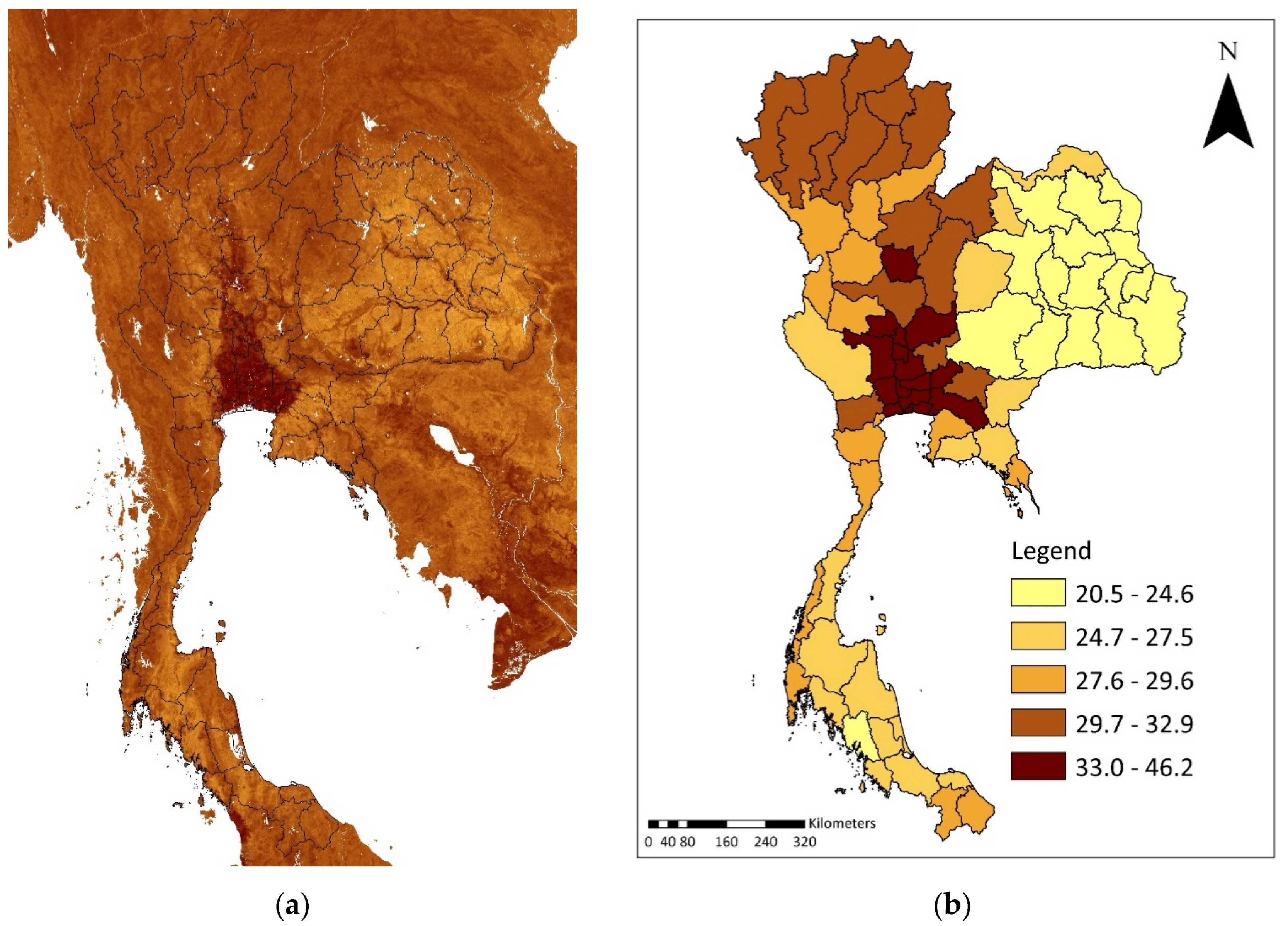
Figure 1 illustrates maps of NTL intensity in Thailand, which are both derived from original data obtained from the Google Earth Engine service along with the transformed provincial NTL index (panels (a) and (b), respectively). These maps show that the highly urbanized provinces include Bangkok and its vicinities.

4.3.3. Localization Economies

Along with the measurement of the urbanization effect, this section details the mathematical construction of the three variables representing localization economies: (1) intra-sectoral knowledge externality (i.e., Marshall–Arrow–Romer spillover); (2) cross-sectoral knowledge externality (i.e., Jacobs spillover); and (3) local intra-sectoral competition externality (i.e., Porter spillover).
Based on information obtained from the IC, the effect of intra-sectoral knowledge externality (i.e., Marshall–Arrow–Romer spillover) is defined as follows:
S p e c i a l i z a t i o n i n d , r , t = E i n d , r , t E r , t
where E i n d , r , t represents total employment of industry i n d in province r in year t ,   and   E r , t is total employment in province r in year t . A higher value of S p e c i a l i z a t i o n i n d , r , t also corresponds to a higher employment share of industry i n d in province r .
Shannon’s entropy was calculated to estimate Jacobs spillover (i.e., the cross-sectoral knowledge externality), indicating the degree of industrial diversity, as mathematically expressed in Equation (16):
D i v e r s i t y r , t = i n d ( E i n d , r , t E r , t l n   E i n d , r , t E r , t   )
where E i n d , r , t denotes total employment of industry i n d in province r in year, and E r , t represents total employment in province r in year t . Finally, we calculated the summation across industries, yielding the value of D i v e r s i t y r , t , which is a measure of the cross-sector knowledge externality of all industries in each province. A higher value of D i v e r s i t y r , t indicates a greater diversity of industries in province r in year t . In contrast, a lower value of Shannon’s entropy suggests a higher specialization of some industries in province r .
The last category of knowledge spillover is the externality arising from competition among industries (i.e., Porter spillover). Equation (17) mathematically defines the formula for quantifying Porter spillover, which can be alternatively recognized as the modification of the Herfindahl–Hirschman Index, as expressed below:
C o m p e t i t i o n i n d , r , t = 1 f ( E f , i n d , r , t E i n d , r , t ) 2
where E f , i n d , r , t is total employment of firm f in industry i n d in year t . The Herfindahl–Hirschman Index represents the summation across firms in each combination of industry and province. A value close to one indicates extreme competition among firms in particular industries. Meanwhile, a value close to zero indicates the extreme concentration of employment in some firms.

4.3.4. Instrumental Variable

As productivity and local density can be simultaneously determined, estimating the agglomeration effect of local density might yield an inconsistent estimation of coefficients. Following the suggestion of Wooldridge (2010), the IV technique was conventionally applied to solve the simultaneity bias, where the validity of IV selection must satisfy both relevance and exogeneity conditions. The latter implies that there should be no correlation between IV and missing variables in the model, and the instrument should not affect the outcome (in this case, regional productivity).
As comprehensively stated in Combes and Gobillon (2015) and in Chen et al. (2022), there are two conditions for selecting the appropriate IV in the empirical estimation of agglomeration elasticity. First, the qualified variable should maintain the inertia of population distribution. Thus, this selected variable should maintain the persistent geographical pattern of urbanization and have a highly positive correlation with the current spatial density of human settlement and economic activity. Second, the selected variable is mathematically orthogonal to the error term, implying that the instrument induces productivity via population density only and does not have other paths of influence.
This study followed the aforementioned recommendations for handling the simultaneity bias. Following Combes et al. (2010), the clay content in soil was used as the instrument variable where the soil content map stood as the instrument in their study examining productivity in the French context. Historically, the clay content in soil was also the most significant factor influencing the early settlement pattern of the Tai ethnic group (the historical ancestors of contemporary Thai people) during the 15th century. As rice cultivation was a major economic endeavor, the formation of cities was mainly determined by the proportion of clay content in the soil. This resulted in the fertile lowlands of the Chao Phraya basin in the central region of Thailand becoming the center of human settlements for centuries (Baker and Phongpaichit 2014).
Moreover, the clay content in the soil does not affect the current locale because land fertility is no longer relevant to economic activity in urban areas dominated by service- and industrial-based sectors (Suphannachart 2017; World Bank 2021). These characteristics therefore satisfy the two conditions in selecting the appropriate IV.
Figure 2 exhibits the spatial distribution of the percentage of soil content. Panel (a) illustrates the raw data obtained from Google Earth Engine (Hengl 2018). Panel (b) shows the geographical pattern of clay content density transformed into the provincial average. The high density of clay content in the central region, suitable for rice cultivation since the 15th century, has nurtured the growth of agricultural-based communities which gradually transformed into the modern-day metropolises of Bangkok and its surroundings.

5. Results

5.1. Descriptive Statistics

This section provides descriptive statistics of the variables used in the first- and second-stage regression. The mean and the standard deviation of each variable for the years 2007, 2012, and 2017, along with the pooled cross-section, are presented in Table 1. From 2007 to 2017, hourly wages (the dependent variable) steadily increased. This increment in hourly wages coincided with a rising proportion of workers with a tertiary education, which increased by around four basis points. Although decreasing, the share of workers without a bachelor’s degree accounted for approximately 88% of the total workers in 2017. This indicates that Thailand’s manufacturing industry has substantially absorbed low-educated workers for decades.
The average age of the sampled workers in 2017 was higher than that of 2007 by a margin of approximately 2.5 years. The proportion of female unemployment in the manufacturing sector has slightly changed. Female labor force participation fell from 52.8% in 2007 to 49.4% in 2017. Table 2 shows that agglomeration measures (population and NTL density) have gradually increased over time. In particular, the increment in NTL density is noticeable, indicating that the density of lights at night was more sensitive to the changes in urban areas than population density. Furthermore, census-based population density often leaves out workers in the informal sector, along with those who seasonally migrate.
Unlike the steady change in the characteristics of workers and local density, the change in the employment structure of the Thai manufacturing sector was relatively stable: the agglomeration measures representing sectoral knowledge externalities—specialization, diversity, and competition—remained relatively stable between 2007 and 2017.
Aside from descriptive statistics, Figure 3 illustrates the change in the spatial distribution of key variables (median hourly wage and population density) between 2007 and 2017. Panels (a) and (b) in Figure 3 show that while workers in the provinces of the central, eastern, and southern regions of Thailand received the highest hourly wages, workers in many provinces in the northern and northeastern regions received the lowest hourly wages. There were also some improvements in recent years as some provinces in the northeastern region progressed to a higher quintile of hourly wage.
Panels (c) and (d) in Figure 3 illustrate the distribution of population density at a provincial level in Thailand. Clearly, provinces in the central and eastern regions of Thailand had the highest population density in both 2007 and 2017. The distribution of population density and hourly wages follow a similar pattern: both the central and eastern regions were the most populous and productive. Overall, Figure 3 shows that hourly wages were highest in most provinces in Thailand’s central and eastern regions, as these areas became more populated.
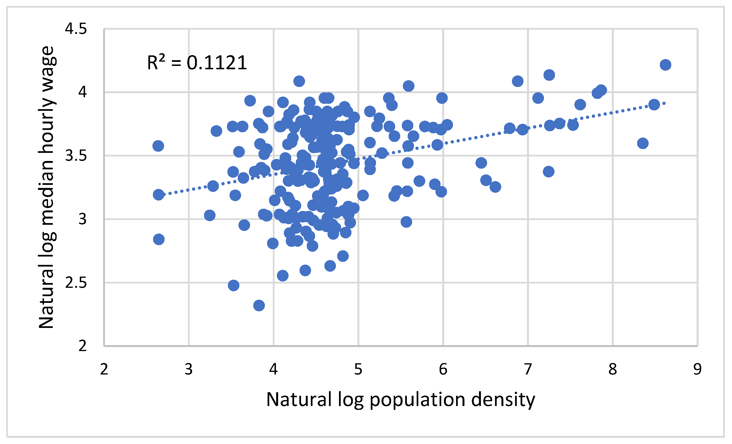
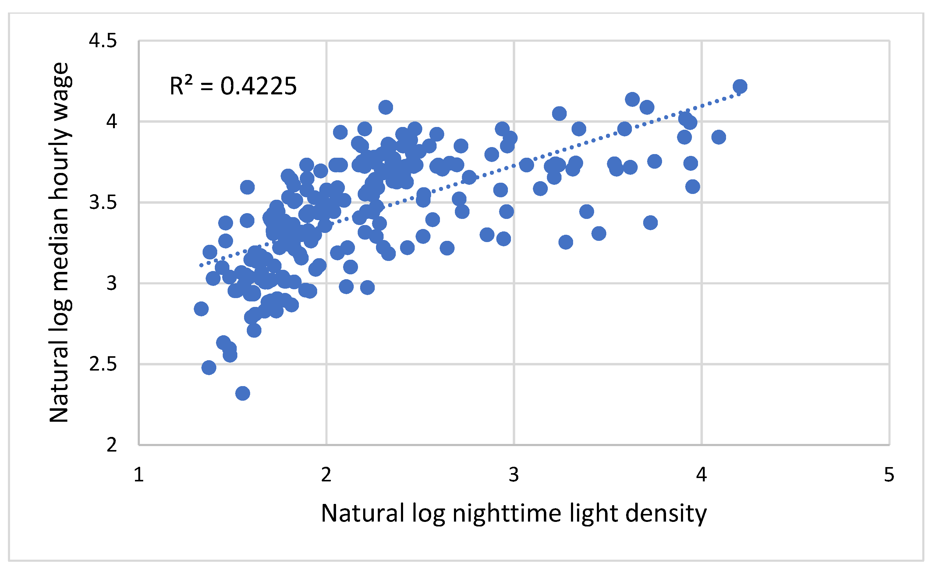
Before discussing the results of the first- and second-stage regression, a simple correlation between the key agglomeration measures of local density and log median hourly wage at the provincial level was plotted, as shown in Figure 4 and Figure 5. Figure 4 shows a positive relationship between population density and median hourly wage with an R-squared of 0.11. A more apparent pattern emerges as NTL density was used as the measure of local density. Figure 5 shows a positive relationship between NTL density and median hourly wage with an R-squared of 0.42. Essentially, NTL density could explain almost half of the variation in the median hourly wage.

5.2. First-Stage Regression Result

The effect of workers’ characteristics on the wage differential was analyzed through the Mincer equation (Equation (11)). Table 3 shows the estimation results for the years 2007, 2012, and 2017 separately, along with the results of the pooled cross-section from 2007 to 2017. Workers with less than a primary education or who had never gone to school were excluded from the regression.
The results suggest that the experience and education of workers have a significant positive effect on their wages. A higher educational level and experience translated into a higher hourly wage. This implied that differences in the composition of workers’ skills among regions affected spatial inequality. The return on tertiary education gradually decreased along with the return on basic education during the 2007–2012 period but slightly increased in 2017. The magnitude and sign of the estimated coefficients for the effects of education and gender are comparable to those in the existing literature (Tangtipongkul 2015; Vivatsurakit and Vechbanyongratana 2020; Warunsiri and McNown 2010). The decreasing return on education was similarly reported by Tangtipongkul (2015). These results confirm the explanatory power of the Mincer equation in wage setting in Thailand, in which the individual characteristics account for roughly 50% of the wage variation. In addition, these obtained coefficients reveal that the gap between the return on high and low education levels has been shrinking. However, the regional wage difference still persists. Thus, the second-stage regression is required, additionally enabling the localized externalities to jointly explain the regional wage difference.

5.3. Second-Stage Regression Result

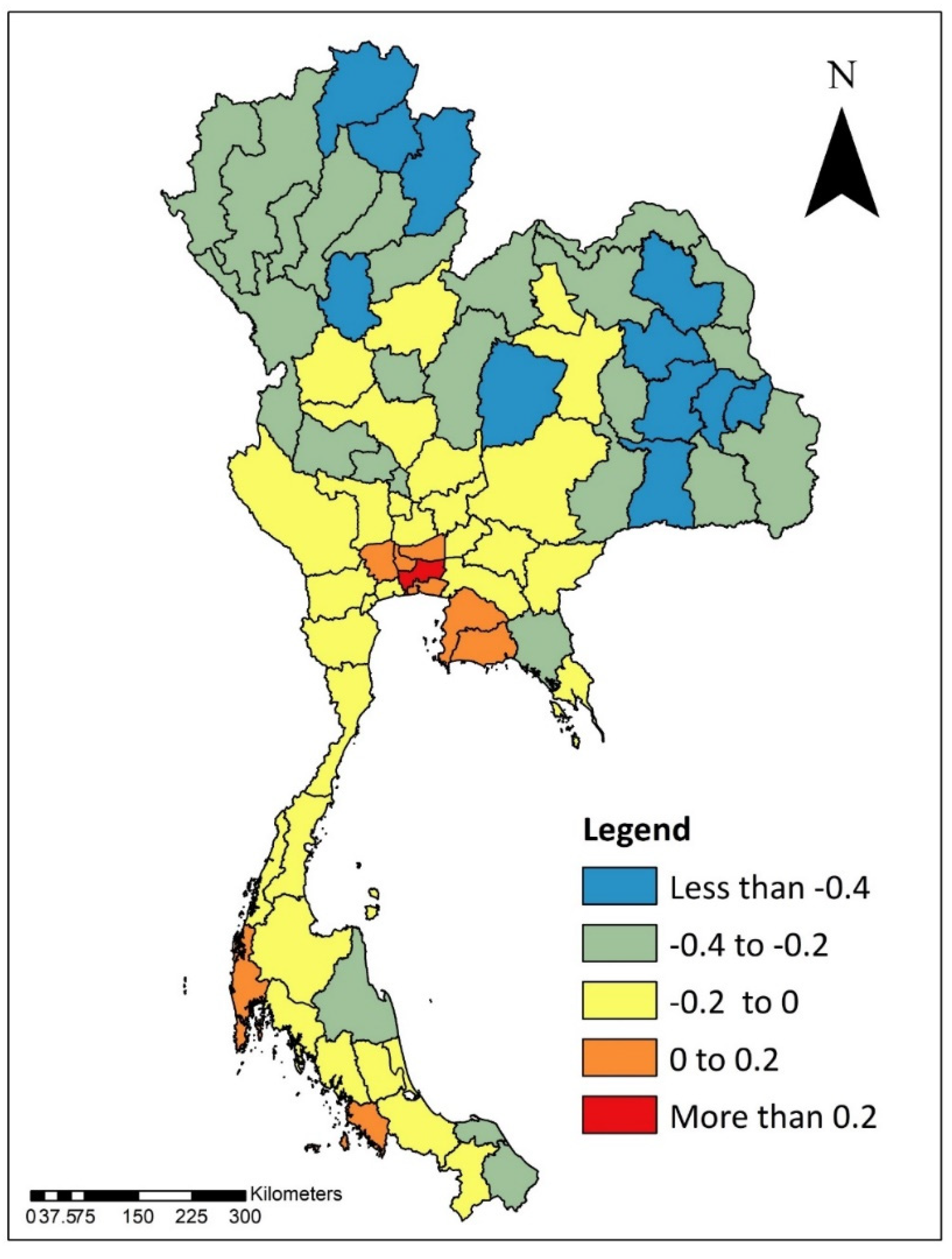
Figure 6 shows the spatial distribution of the average spatial residual by province. Following Groot et al. (2014), the spatial residuals at the provincial level shown in Figure 6 are interpreted as an average regional wage (after controlling for the observed worker characteristics and sectoral composition). Alternatively, the provincial average spatial residual could also be recognized as a regional wage premium (Ridhwan 2021). To simplify the interpretation, the nationwide average value was used for normalizing the spatial residuals.
Figure 6 illustrates that after controlling for skill and experience, workers in the Bangkok Metropolitan Region (highlighted in red) and those in the eastern and southern regions (highlighted in orange) earn a higher wage premium. In particular, the geographical distribution pattern of the obtained spatial residuals is similar to those of the Netherlands and Indonesia, where Amsterdam and Jakarta are associated with the highest wage premium, respectively (Groot et al. 2014; Ridhwan 2021).
Table 4 presents the second-stage regression results of the OLS and IV methods. According to the OLS technique, doubling the population density results in a 10% increase in wages. The effect of local density on wages rises to 19% in the IV estimate, indicating that endogeneity does not result in an upward bias in the OLS estimate. Other studies similarly found that the IV estimate leads to an increase in the magnitude of the effect of local density on wages (Barufi et al. 2016; Combes et al. 2008; Groot and de Groot 2020; Groot et al. 2014; Ridhwan 2021).
The agglomeration effect in Thailand is comparable to the agglomeration effect found in other developing countries such as India, China, Colombia, and Brazil (Barufi et al. 2016; Chauvin et al. 2017; Duranton 2016). Other studies have found that Thailand’s agglomeration effects at the provincial level range between 16% and 37% (Limpanonda 2012).
The effect of local density on wages in Thailand was found to be greater than the effect of local density on wages in developed countries such as the Netherlands and France, where the impact of local density on wages was reported to be approximately 4–5% (Combes et al. 2008; Groot et al. 2014). Nevertheless, numerous factors could affect the degree of agglomeration, including the spatial scale and model specifications (Combes and Gobillon 2015; Grover et al. 2021). The agglomeration effect in the Netherlands doubled when the unit of analysis was changed from municipalities to NUTS-3 regions (Groot et al. 2014). Through meta-analysis, Grover et al. (2021) showed a higher gross agglomeration effect in developing countries. However, when the increasing congestion in developing countries is considered, the size of the agglomeration effect dramatically drops to the level seen in developed economies.
Regarding the effect of localization economies, specialization (i.e., MAR spillover) is found to have no effect on workers’ wages. The insignificance of specialization is also found in Brazil’s manufacturing sector (Barufi et al. 2016). Combes et al. (2008) demonstrated via spatial variance analysis that while overall employment density explains a significant portion of the regional inequalities in productivity, the explanatory power of specialization is rather minute. Meanwhile, IV method results indicate that diversity is negatively associated with spatial residuals, suggesting that cross-sectoral knowledge externality does not follow the theory of Jacobs spillover. This result coincides with findings from France, the Netherlands, Indonesia, and Brazil (Barufi et al. 2016; Combes et al. 2008; Groot et al. 2014; Ridhwan 2021).
For the last category of externality (i.e., Porter spillover), the obtained coefficient of competition is negative and statistically significant, similar to the empirical findings from Brazil and the Netherlands (Barufi et al. 2016; Groot et al. 2014). On the other hand, the ambiguity of the localization effect is also reported by Combes and Gobillon (2015).
The result of the Durbin–Wu–Hausman test (Table 5) indicates that population density is clearly an endogenous variable. The high values of the Durbin–Wu–Hausman statistics support our rationale for using two-stage least squares regression. Moreover, Table 6 shows that the instrument is relevant. The high F statistics suggest that the instrument is valid for predicting current population density.

5.4. The NTL Intensity

Table 7 shows the results of the second-stage regression that used NTL intensity as a proxy for local density. Essentially, Table 7 is a re-estimation of Equation (17), but the population density is substituted with NTL intensity. It shows that when population density is replaced by NTL intensity, the results remain robust.
The coefficient of NTL intensity in the IV model yields slightly less value than the OLS estimate, suggesting that OLS has not resulted in a downward bias. According to the IV estimate, the magnitude of the agglomeration effect is larger than in the previous model (22% versus 19%). As NTL intensity captures the actual density in the urban areas of Thailand, this result suggests that the agglomeration effect is stronger for informal workers, such as seasonal migrants, and urban informal labor. This result is not unique to Thailand. Similarly, informal workers in Colombia also benefit more from agglomeration economies (Duranton 2016).
The effect of specialization also remains insignificant. Diversity negatively affects spatial residuals, as it did in the previous model, but at a lower magnitude and significance level. Unlike the previous results, the effect of competition becomes insignificant in this model. These regression results reveal the decomposed components of agglomeration effects. In particular, specialization and competition are not statistically insignificant, implying that the spatial concentration of industry and the local intensity of competition in Thailand have been inadequate to induce agglomeration externalities. As previously stated, these outcomes are similar to the findings in some developing countries, where the concentration of low-technology production and the imperfect market mechanism in some areas are conventionally observed. Hence, technological development and other fundamentals (e.g., enforcement of competition law) are also important underlying factors inducing agglomeration effects.
Table 8 shows that the coefficient value of NTL intensity in the IV estimate is not significantly different from that of the OLS estimate. This implies that using NTL intensity as a proxy for local density circumvents the endogeneity bias. Table 9 shows that the percentage of clay content in soil is not a weak instrument in the model with NTL intensity.
All the obtained results indicate that applying the two-stage regression technique to the data set, which is a combination of official surveys and geospatial indicators, can quantitatively reveal the factors influencing the regional wage differences in Thailand. In particular, although using different combinations of population density proxies and regression techniques, the main finding is robust, confirming the effect of agglomeration economies on labor productivity. Thus, in the case of Thailand, the unique pattern of high wage concentration in Bangkok and its surroundings is the consequence of a high agglomeration force induced by high population density. From a nationwide perspective, this also causes the regional inequality of income.

5.5. Policy Recommendations

As initially stated, Thailand has experienced declining GDP growth and persistent spatial inequality. The main findings of this study suggest policy recommendations that could mitigate both these problems. Specifically, the estimated coefficients of agglomeration elasticity signify the productivity enhancement arising from density-led externalities. Driven by Bangkok-centric growth for centuries, the Thai economy should alternatively create multipolar growth in all regions. It is highly recommended that the new development plan should facilitate decentralized growth empowered by establishing new cities that create high agglomeration externalities. The degree of agglomeration elasticity obtained herein will also ensure regional growth potential induced by the simultaneous increment in productivity and wages. The expansion of high agglomeration cities in multiple regions will lessen the urban primacy of Bangkok and will ultimately lift the nationwide average income.

5.6. Limitations

The limitations of this paper are four-fold (and are also key issues for future research). First, the spatial resolution should be refined to a smaller scale of geographical boundary (such as district or sub-district), yielding more analytical details. Second, the frequency of data should be higher. In particular, productivity can alternatively be derived from the annual or quarterly financial statements of firms. This aspect is subsequently related to the third limitation on static analysis. The availability of high-frequency and continuous data sets enables the creation of a dynamic analytical framework, revealing the intertemporal relationship between density and agglomeration (Glaeser and Maré 2001; Wheeler 2006; Yankow 2006; De La Roca and Puga 2012). The last limitation is the variety of production sectors. For decades, technological revolutions have resulted in the innovation of new products and services. Thus, the analysis should include new sectors, particularly those related to information technology (Massimino et al. 2017; Jang et al. 2017).

6. Conclusions

This study examined the causes of persistent spatial inequality in Thailand. The two-stage estimation method was utilized to examine how agglomeration externalities affect the difference in productivity between regions. This work also innovatively utilized open geospatial data and satellite-based indicators. In particular, NTL intensity was used as a proxy for local density, and the percentage of clay content in soil was applied as an instrumental variable.
The estimation results suggest that heterogeneity in worker competence and agglomeration externalities could explain the regional wage differentials. Accordingly, besides individual skills, workers in highly urbanized areas also benefit from agglomeration externalities. These findings coincide with previous studies on developing and developed economies, recommending a new policy of redistributing economic growth by establishing regional cities that create density-led spillovers.
The limitations of this study include the un-updated industrial classification and the spatio-temporal resolutions of data. To overcome these restrictions, future research should enhance the spatial and temporal details of the data, along with the inclusion of new industries. Finally, a dynamic analytical approach should be applied to examine the multi-period influences of agglomeration externalities.

Author Contributions

Conceptualization, N.P. (Nutchapon Prasertsoong) and N.P. (Nattapong Puttanapong); methodology, N.P. (Nutchapon Prasertsoong) and N.P. (Nattapong Puttanapong); software, N.P. (Nutchapon Prasertsoong); validation, N.P. (Nattapong Puttanapong); formal analysis, N.P. (Nutchapon Prasertsoong) and N.P. (Nattapong Puttanapong); investigation, N.P. (Nattapong Puttanapong); resources, N.P. (Nutchapon Prasertsoong); data curation, N.P. (Nutchapon Prasertsoong); writing—original draft preparation, N.P. (Nutchapon Prasertsoong); writing—review and editing, N.P. (Nattapong Puttanapong); visualization, N.P. (Nutchapon Prasertsoong); supervision, N.P. (Nattapong Puttanapong); project administration, N.P. (Nattapong Puttanapong); funding acquisition, N.P. (Nutchapon Prasertsoong) All authors have read and agreed to the published version of the manuscript.

Funding

Thammasat University (Doctoral Scholarship for Research).

Informed Consent Statement

Not applicable.

Data Availability Statement

Not applicable.

Conflicts of Interest

The authors declare no conflict of interest. The funders had no role in the design of the study; in the collection, analyses, or interpretation of data; in the writing of the manuscript, or in the decision to publish the results.

Appendix A

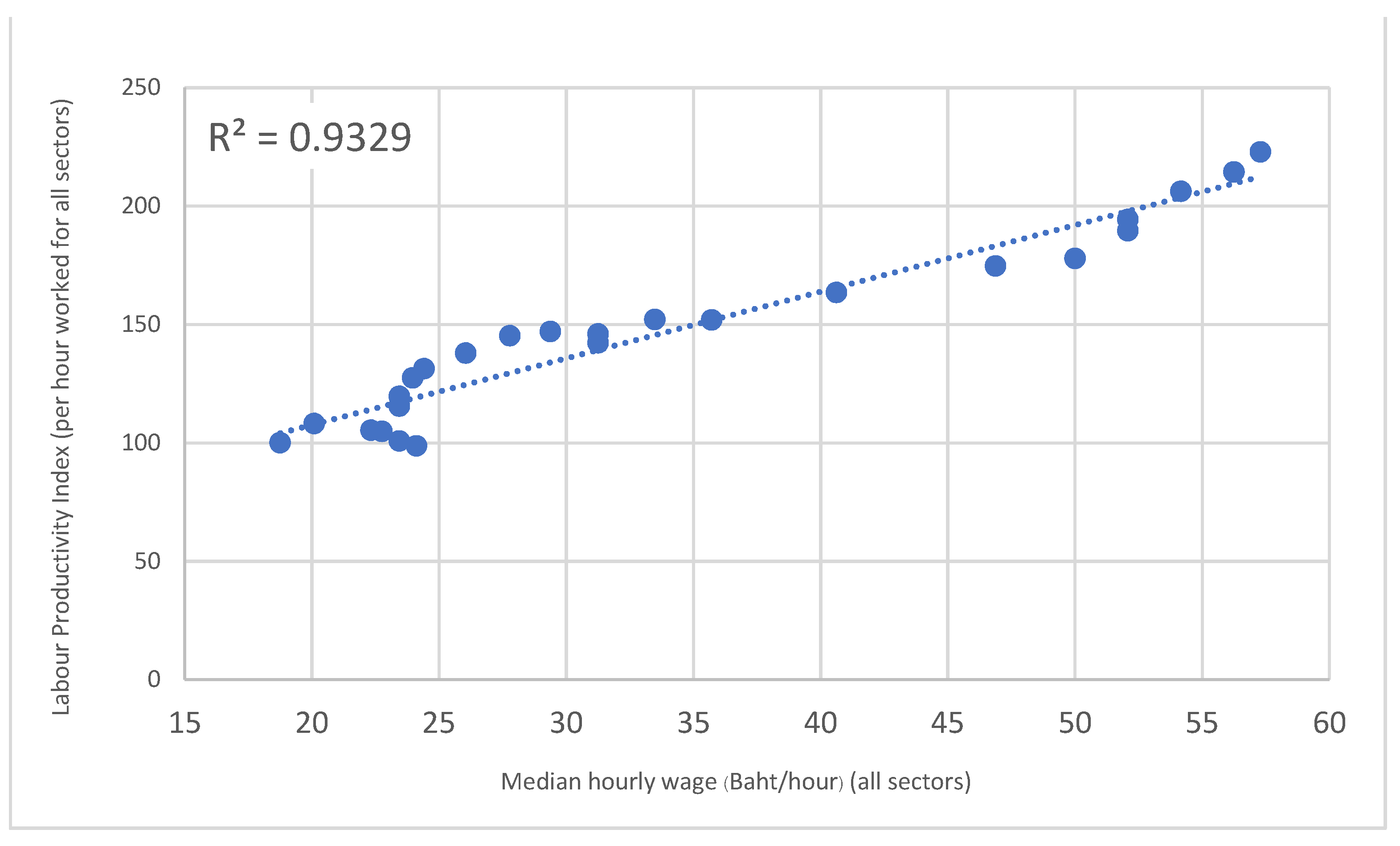
Figure A1 and Figure A2 exhibit the statistically significant relationship between wages and labor productivity in Thailand during the 1995–2020 period. The labor productivity index, representing the hourly output per worker, was calculated by the Bank of Thailand, and the hourly wage was obtained from the LFS. Specifically, Figure A1 shows the regression result between median hourly wage and hourly productivity, which obtains a high R-squared value. Alternatively, Figure A2 indicates the regression result between the average hourly wage and hourly labor productivity, which also yields a high magnitude of R-squared. These results affirm the validity of using the hourly wage as a proxy of hourly labor productivity.
Figure A1. Correlation between labor productivity and the median hourly wage (Baht/hour), 1995–2020.
Economies 10 00319 g0a1
Figure A2. Correlation between labor productivity and average hourly wage (Baht/hour), 1995–2020.
Economies 10 00319 g0a2

References

  1. Amare, Mulubrhan, Lena Hohfeld, Somchai Jitsuchon, and Hermann Waibel. 2012. Rural–Urban Migration and Employment Quality: A Case Study from Thailand. Asian Development Bank Economics Working Paper Series No. 309. Manila: Asian Development Bank. [Google Scholar]
  2. Arrow, Kenneth. 1962. Economic welfare and the allocation of resources for invention. In The Rate and Direction of Inventive Activity: Economic and Social Factors. Princeton: Princeton University Press, pp. 609–26. [Google Scholar]
  3. Baker, Chris, and Pasuk Phongpaichit. 2014. A History of Thailand, 3rd ed. Cambridge: Cambridge University Press. [Google Scholar]
  4. Barufi, Ana Maria Bonomi, Eduardo Amaral Haddad, and Peter Nijkamp. 2016. Industrial scope of agglomeration economies in Brazil. Annals of Regional Science 56: 707–55. [Google Scholar] [CrossRef] [Green Version]
  5. Baum-Snow, Nathaniel, and Fernando Ferreira. 2015. Chapter 1—Causal Inference in Urban and Regional Economics. In Handbook of Regional and Urban Economics. Edited by Gilles J. Duranton, Vernon Henderson and William C. Strange. Amsterdam: Elsevier, pp. 3–68. [Google Scholar]
  6. Beaudry, Catherine, and Andrea Schiffauerova. 2009. Who’s right, Marshall or Jacobs? The localization versus urbanization debate. Research Policy 38: 318–37. [Google Scholar] [CrossRef] [Green Version]
  7. Buchanan, James. 1965. An economic theory of clubs. Economica 32: 1–14. [Google Scholar] [CrossRef]
  8. Chauvin, Juan Pablo, Edward Glaeser, Yueran Ma, and Kristina Tobio. 2017. What is different about urbanization in rich and poor countries? Cities in Brazil, China, India and the United States. Journal of Urban Economics 98: 17–49. [Google Scholar] [CrossRef] [Green Version]
  9. Chen, Liming, Rana Hasan, and Yi Jiang. 2022. Urban Agglomeration and Firm Innovation: Evidence from Asia. The World Bank Economic Review 36: 533–58. [Google Scholar] [CrossRef]
  10. Ciccone, Antonio, and Robert E. Hall. 1996. Productivity and the Density of Economic Activity. The American Economic Review 86: 54–70. [Google Scholar]
  11. Combes, Pierre-Philippe, and Laurent Gobillon. 2015. Chapter 5—The Empirics of Agglomeration Economies. In Handbook of Regional and Urban Economics. Edited by Gilles J. Duranton, Vernon Henderson and William C. Strange. Amsterdam: Elsevier, pp. 247–348. [Google Scholar]
  12. Combes, Pierre-Philippe, Gilles Duranton, and Laurent Gobillon. 2008. Spatial wage disparities: Sorting matters! Journal of Urban Economics 63: 723–42. [Google Scholar] [CrossRef] [Green Version]
  13. Combes, Pierre-Philippe, Gilles Duranton, and Laurent Gobillon. 2011. The identification of agglomeration economies. Journal of Economic Geography 11: 253–66. [Google Scholar] [CrossRef] [Green Version]
  14. Combes, Pierre-Philippe, Gilles Duranton, Laurent Gobillon, and Sébastien Roux. 2010. Estimating agglomeration economies with history, geology, and worker effects. In Agglomeration Economics. Chicago: University of Chicago Press, pp. 15–66. [Google Scholar]
  15. de Groot, Henri L. F., Jacques Poot, and Martijn J. Smit. 2009. Chapter 14: Agglomeration Externalities, Innovation and Regional Growth: Theoretical Perspectives and Meta-Analysis. In Handbook of Regional Growth and Development Theories. Cheltenham: Edward Elgar Publishing. [Google Scholar]
  16. De La Roca, Jorge, and Diego Puga. 2012. Learning by Working in Big Cities. Available online: https://ssrn.com/abstract=2210212 (accessed on 15 March 2022).
  17. Dixon, Chris J. 1999. The Thai Economy: Uneven Development and Internationalisation. London: Routledge. [Google Scholar]
  18. Duranton, Gilles. 2014. Growing through Cities in Developing Countries. The World Bank Research Observer 30: 39–73. [Google Scholar] [CrossRef] [Green Version]
  19. Duranton, Gilles. 2016. Agglomeration Effects in Colombia. Journal of Regional Science 56: 210–38. [Google Scholar] [CrossRef]
  20. Duranton, Gilles, and Diego Puga. 2004. Chapter 48—Micro-Foundations of Urban Agglomeration Economies. In Handbook of Regional and Urban Economics. Edited by J. Vernon Henderson and Jacques-François Thisse. Amsterdam: Elsevier, pp. 2063–117. [Google Scholar]
  21. Fujita, Masahisa, Paul Krugman, and Tomoya Mori. 1999. On the evolution of hierarchical urban systems. European Economic Review 43: 209–51. [Google Scholar] [CrossRef]
  22. Glaeser, Edward L., and David C. Maré. 2001. Cities and Skills. Journal of Labor Economics 19: 316–42. [Google Scholar] [CrossRef]
  23. Glaeser, Edward L., Hedi D. Kallal, José A. Scheinkman, and Andrei Shleifer. 1992. Growth in Cities. Journal of Political Economy 100: 1126–52. [Google Scholar] [CrossRef]
  24. Groot, Stefan P. T., and Henri L. F. de Groot. 2020. Estimating the Skill Bias in Agglomeration Externalities and Social Returns to Education: Evidence from Dutch Matched Worker-Firm Micro-Data. De Economist 168: 53–78. [Google Scholar] [CrossRef] [Green Version]
  25. Groot, Stefan P. T., Henri L. F. de Groot, and Martijn J. Smit. 2014. Regional Wage Differences in the Netherlands: Micro Evidence on Agglomeration Externalities. Journal of Regional Science 54: 503–23. [Google Scholar] [CrossRef] [Green Version]
  26. Grover, Arti, Somik V. Lall, and Jonathan Timmis. 2021. Agglomeration Economies in Developing Countries. Policy Research Working Paper 9730. Washington, DC: Word Bank Group. [Google Scholar]
  27. Henderson, J. Vernon. 1986. Efficiency of resource usage and city size. Journal of Urban Economics 19: 47–70. [Google Scholar] [CrossRef]
  28. Henderson, J. Vernon, and Sebastian Kriticos. 2018. The Development of the African System of Cities. Annual Review of Economics 10: 287–314. [Google Scholar] [CrossRef]
  29. Henderson, Vernon. 2003. The Urbanization Process and Economic Growth: The So-What Question. Journal of Economic Growth 8: 47–71. [Google Scholar] [CrossRef]
  30. Hengl, Tomislav. 2018. Clay Content in % (kg/kg) at 6 Standard Depths (0, 10, 30, 60, 100 and 200 cm) at 250 m Resolution. Zenodo. Available online: https://scholar.google.com.hk/scholar?hl=en&as_sdt=0%2C5&q=10.5281%2Fzenodo.1476854&btnG= (accessed on 15 March 2022).
  31. Houbcharaun, Akarapon. 2013. Essays on Economic Liberalization and Spatial Economics. Honolulu: University of Hawai’i. [Google Scholar]
  32. Huang, Qingxu, Xi Yang, Bin Gao, Yang Yang, and Yuanyuan Zhao. 2014. Application of DMSP/OLS Nighttime Light Images: A Meta-Analysis and a Systematic Literature Review. Remote Sensing 6: 6844–66. [Google Scholar] [CrossRef] [Green Version]
  33. Jacobs, Jane. 1969. The Economy of Cities. New York: Random House. [Google Scholar]
  34. Jang, Seongsoo, Jinwon Kim, and Max von Zedtwitz. 2017. The importance of spatial agglomeration in product innovation: A microgeography perspective. Journal of Business Research 78: 143–54. [Google Scholar] [CrossRef]
  35. Kelley, Kevin C. 1977. Urban disamenities and the measure of economic welfare. Journal of Urban Economics 4: 379–88. [Google Scholar] [CrossRef]
  36. Krugman, Paul. 1999. The Role of Geography in Development. International Regional Science Review 22: 142–61. [Google Scholar] [CrossRef] [Green Version]
  37. Li, Deren, Xia Zhao, and Xi Li. 2016. Remote sensing of human beings—A perspective from nighttime light. Geospatial Information Science 19: 69–79. [Google Scholar] [CrossRef] [Green Version]
  38. Limpanonda, Suphannada. 2012. Provincial Disparities in Thailand: Convergence, Agglomeration Economies and Effects on Poverty, 1988–2008. London: SOAS, University of London. [Google Scholar]
  39. Lucas, Robert. 1988. On the mechanics of economic development. Journal of Monetary Economics 22: 3–42. [Google Scholar] [CrossRef]
  40. Marshall, Alfred. 1890. Principles of Economics Macmillan, 8th ed. London: Macmillan. First published in 1920. [Google Scholar]
  41. Massimino, Brett, John V. Gray, and Kenneth K. Boyer. 2017. The Effects of Agglomeration and National Property Rights on Digital Confidentiality Performance. Production and Operations Management 26: 162–79. [Google Scholar] [CrossRef]
  42. Melo, Patricia C., Daniel J. Graham, and Robert B. Noland. 2009. A meta-analysis of estimates of urban agglomeration economies. Regional Science and Urban Economics 39: 332–42. [Google Scholar] [CrossRef] [Green Version]
  43. Mincer, Jacob. 1974. Schooling, Earnings, and Experience. New York: Columbia University Press. [Google Scholar]
  44. Moomaw, Ronald L. 1981. Productivity and City Size: A Critique of the Evidence. The Quarterly Journal of Economics 96: 675–88. [Google Scholar] [CrossRef]
  45. Moomaw, Ronald L. 1998. Agglomeration economies: Are they exaggerated by industrial aggregation? Regional Science and Urban Economics 28: 199–211. [Google Scholar] [CrossRef]
  46. Nakamura, Ryohei. 1985. Agglomeration economies in urban manufacturing industries: A case of Japanese cities. Journal of Urban Economics 17: 108–24. [Google Scholar] [CrossRef]
  47. Poonsab, Wissanee, Joann Vanek, and Françoise Carré. 2019. Informal Workers in Urban Thailand: A statistical Snapshot. WIEGO Statistical Brief 20: 2–4. [Google Scholar]
  48. Porter, Michael E. 1990. The Competitive Advantage of Nations. Houndmills: Macmillan. [Google Scholar]
  49. Puga, Diego. 2010. The Magnitude and Causes of Agglomeration Economies. Journal of Regional Science 50: 203–19. [Google Scholar] [CrossRef] [Green Version]
  50. Puttanapong, Nattapong. 2008. The Computable General Equilibrium (CGE) Models with Monte-Carlo Simulation for Thailand: An Impact Analysis of Baht Appreciation. Ithaca: Cornell University. [Google Scholar]
  51. Puttanapong, Nattapong. 2018. Monocentric Growth and Productivity Spillover in Thailand. Bangkok: Institute of Developing Economies, Japan External Trade Organization. [Google Scholar]
  52. Puttanapong, Nattapong, Amornrat Luenam, and Pit Jongwattanakul. 2022a. Spatial Analysis of Inequality in Thailand: Applications of Satellite Data and Spatial Statistics/Econometrics. Sustainability 14: 3946. [Google Scholar] [CrossRef]
  53. Puttanapong, Nattapong, Arturo Martinez, Joseph A. Bulan, Mildred Addawe, Ron L. Durante, and Marymell Martillan. 2022b. Predicting Poverty Using Geospatial Data in Thailand. ISPRS International Journal of Geo-Information 11: 293. [Google Scholar] [CrossRef]
  54. Richter, Kaspar. 2006. Thailand’s Growth Path: From Recovery to Prosperity. Policy Research Working Paper No. 3912. Washington, DC: World Bank. [Google Scholar]
  55. Ridhwan, Masagus M. 2021. Spatial wage differentials and agglomeration externalities: Evidence from Indonesian microdata. Economic Analysis and Policy 71: 573–91. [Google Scholar] [CrossRef]
  56. Romer, Paul M. 1986. Increasing Returns and Long-Run Growth. Journal of Political Economy 94: 1002–37. [Google Scholar] [CrossRef] [Green Version]
  57. Rosenthal, Stuart S., and William C. Strange. 2004. Chapter 49—Evidence on the Nature and Sources of Agglomeration Economies. In Handbook of Regional and Urban Economics. Edited by J. Vernon Henderson and Jacques-François Thisse. Amsterdam: Elsevier, pp. 2119–71. [Google Scholar]
  58. Sangkasem, Krittaya, and Nattapong Puttanapong. 2022. Analysis of spatial inequality using DMSP-OLS nighttime-light satellite imageries: A case study of Thailand. Regional Science Policy & Practice 14: 828–49. [Google Scholar] [CrossRef]
  59. Short, John Rennie, and Luis Mauricio Pinet-Peralta. 2009. Urban Primacy: Reopening the Debate. Geography Compass 3: 1245–66. [Google Scholar] [CrossRef]
  60. Southichack, Mana Kayne. 1998. Regional Convergence and Agglomeration Economies: The Case of Thailand. Honolulu: University of Hawaii. [Google Scholar]
  61. Stock, James, and Motohiro Yogo. 2005. Asymptotic distributions of instrumental variables statistics with many instruments. Identification and Inference for Econometric Models: Essays in Honor of Thomas Rothenberg 6: 109–20. [Google Scholar]
  62. Suphannachart, Waleerat. 2017. What drives labour productivity in the ageing agriculture of Thailand? Advances in Management and Applied Economics 7: 89. [Google Scholar]
  63. Suttiwichienchot, Autsawin, and Nattapong Puttanapong. 2014. A Study on Internal Labor Movement and Policy Multiplier in Thailand. Eurasian Journal of Economics and Finance 2: 57–68. [Google Scholar] [CrossRef]
  64. Sveikauskas, Leo. 1975. The Productivity of Cities. The Quarterly Journal of Economics 89: 393–413. [Google Scholar] [CrossRef]
  65. Tangtipongkul, Kaewkwan. 2015. Rates of Return to Schooling in Thailand. Asian Development Review 32: 38–64. [Google Scholar] [CrossRef]
  66. Tippakoon, Phakpoom. 2011. Industrial Agglomeration and Labor Productivity: Evidence from Manufacturing Establishments in Thailand. Southeast Asian Journal of Economics 23: 39–76. [Google Scholar]
  67. Vivatsurakit, Tanthaka, and Jessica Vechbanyongratana. 2020. Returns to education among the informally employed in Thailand. Asian-Pacific Economic Literature 34: 26–43. [Google Scholar] [CrossRef]
  68. Warunsiri, Sasiwimon, and Robert McNown. 2010. The Returns to Education in Thailand: A Pseudo-Panel Approach. World Development 38: 1616–25. [Google Scholar] [CrossRef]
  69. Wheeler, Christopher H. 2006. Cities and the growth of wages among young workers: Evidence from the NLSY. Journal of Urban Economics 60: 162–84. [Google Scholar] [CrossRef] [Green Version]
  70. Wooldridge, Jeffrey M. 2010. Econometric Analysis of Cross Section and Panel Data. Cambridge: MIT Press. [Google Scholar]
  71. World Bank. 2021. Employment in Agriculture (% of Total employment) (Modeled ILO Estimate)—Thailand. Washington, DC: World Bank. [Google Scholar]
  72. Yankow, Jeffrey J. 2006. Why do cities pay more? An empirical examination of some competing theories of the urban wage premium. Journal of Urban Economics 60: 139–61. [Google Scholar] [CrossRef]
  73. Zhang, Qingling, and Karen C. Seto. 2011. Mapping urbanization dynamics at regional and global scales using multi-temporal DMSP/OLS nighttime light data. Remote Sensing of Environment 115: 2320–29. [Google Scholar] [CrossRef]
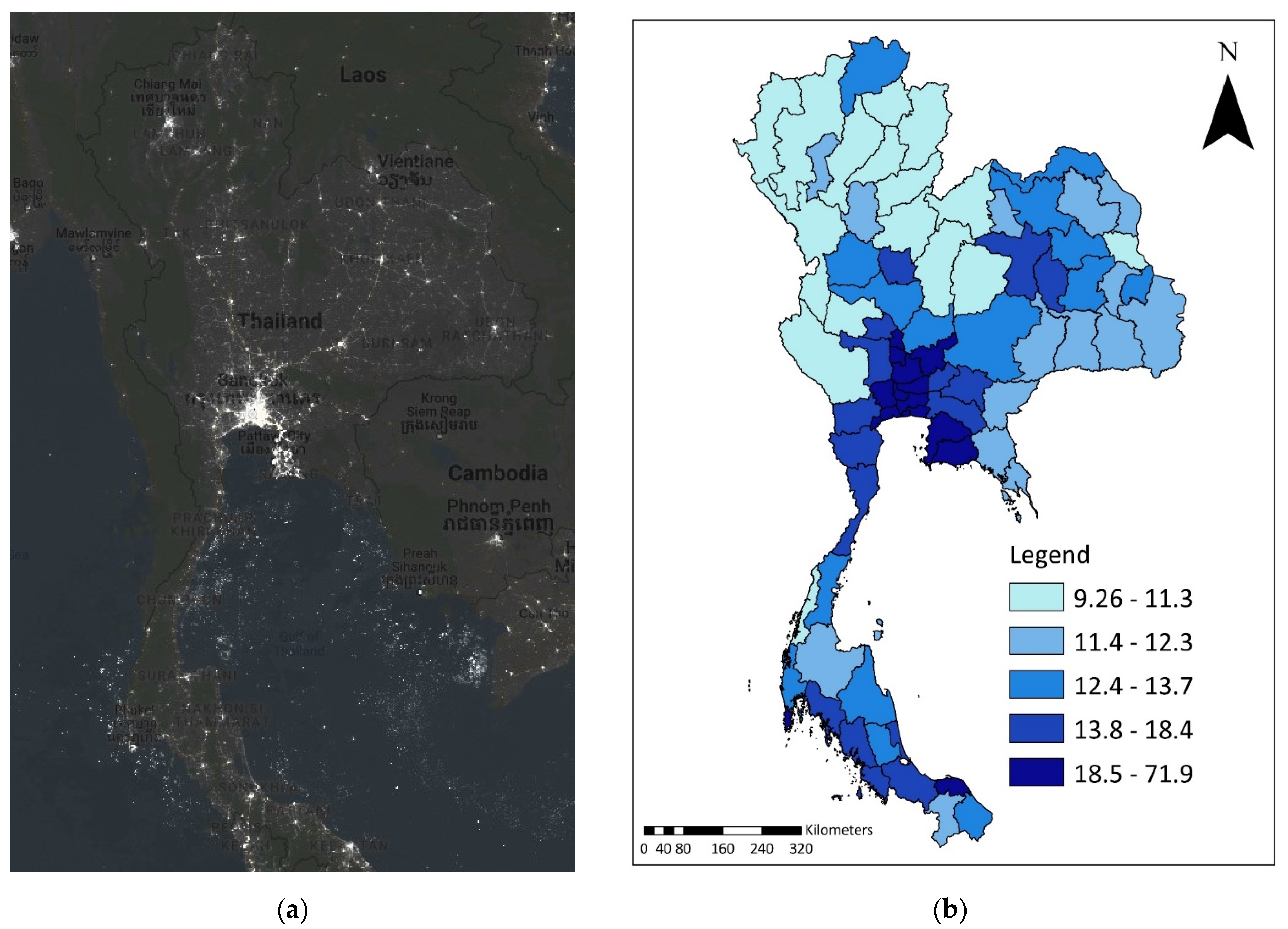
Figure 1. Comparison between original nighttime light (NTL) data and transformed data in 2021: (a) original data; (b) transformed data.
Economies 10 00319 g001
Figure 2. Comparison between original data of the percentage of clay content and transformed data: (a) original data; (b) transformed data.
Economies 10 00319 g002
Figure 3. Comparison of median log hourly wage and population density in 2007 and 2017: (a) median log hourly wage in 2007; (b) median log hourly wage in 2017; (c) log population density (person per square kilometer) in 2007; (d) log population density (person per square kilometer) in 2017.
Economies 10 00319 g003
Figure 4. Relationship between population density and median hourly wage at the provincial level, 2007 to 2017.
Economies 10 00319 g004
Figure 5. Relationship between night-time light density and median hourly wage at the provincial level, 2007 to 2017.
Economies 10 00319 g005
Figure 6. The average spatial residual by province, 2007–2017.
Economies 10 00319 g006
Table 1. Descriptive statistics of variables in first-stage regression.
First-Stage Regression200720122017Pooled
Observations12,40312,37410,45335,230
Continuous variables
Log hourly wage3.323.703.933.63
(0.66)(0.50)(0.50)(0.64)
Age34.6635.2237.0535.56
(11.11)(10.49)(11.08)(10.93)
Categorical variables
Female52.75%50.83%49.44%51.06%
Less than primary—post secondary education92.44%90.36%88.57%90.56%
Tertiary education7.55%9.63%11.42%9.43%
Notes: Standard deviations are shown in parentheses.
Table 2. Descriptive statistics of variables in second-stage regression.
Second-Stage Regression200720122017Pooled
Observations7149499662629
Log population density4.955.015.065.06
(1.07)(1.11)(1.17)(1.12)
Log nighttime light density2.142.392.682.43
(0.7)(0.71)(0.55)(0.69)
Specialization 0.100.070.070.08
(0.13)(0.11)(0.11)(0.11)
Diversity1.732.112.092.00
(0.30)(0.50)(0.44)(0.45)
Competition0.750.760.770.76
(0.24)(0.25)(0.24)(0.24)
Notes: Standard deviations are shown in parentheses.
Table 3. Results of Mincer regression (Equation (11)).
Variables200720122017Pooled 2007, 2012, and 2017
Age0.0537 ***0.0427 ***0.0319 ***0.0438 ***
(27.31)(10.53)(16.62)(38.27)
Age squared−0.000563 ***−0.000468 ***−0.000308 ***−0.000464 ***
(−22.92)(−17.84)(−12.69)(−31.77)
Female−0.197 ***−0.150 ***−0.159 ***−0.175 ***
(−21.85)(−19.34)(−21.72)(−36.63)
Education Dummies
Primary0.148 ***0.0878 ***0.111 ***0.118 ***
(9.99)(6.57)(8.64)(14.93)
Lower secondary0.269 ***0.181 ***0.184 ***0.217 ***
(16.72)(12.97)(14.05)(26.03)
Upper secondary0.397 ***0.275 ***0.294 ***0.330 ***
(24.01)(19.36)(22.12)(38.68)
Post-secondary education0.676 ***0.494 ***0.495 ***0.561 ***
(31.58)(28.36)(30.48)(52.36)
Bachelor’s degree1.165 ***0.943 *** 0.894 ***1.002 ***
(56.38)(55.39)(58.33)(97.25)
Graduate (Master and PhD)1.979 ***1.528 ***1.423 ***1.636 ***
(32.32)(34.91)(33.25)(56.74)
Constant2.354 ***2.952 ***3.291 ***2.604 ***
(52.22)(73.82)(85.74)(107.69)
Industry dummiesIncludedIncludedIncludedIncluded
Year dummiesNot IncludedNot IncludedNot IncludedNot Included
Province dummiesIncludedIncludedIncludedIncluded
R squared0.4920.4920.5120.555
Number of observations12,40312,37410,45335,230
Notes: Education dummies denote the highest qualification obtained. The omitted education category is those workers who have less than a primary education; t and z statistics in parentheses; * p < 0.05, ** p < 0.01, *** p < 0.001.
Table 4. Results of the second-stage regression with population density as a proxy for local density.
VariablesOLS2SLS
Log population density0.10 ***0.19 ***
(11.64)(5.75)
Specialization−0.010.03
(−0.16)(0.37)
Diversity−0.03−0.12 **
(−1.56)(−3.18)
Competition−0.03−0.10 *
(−0.93)(−2.47)
Area6.94×10-70.0000106 **
(0.42)(2.70)
Constant−0.85 ***−1.14 ***
(−14.84)(−9.66)
Industry dummiesIncludedIncluded
Year dummiesIncludedIncluded
R squared0.350.33
Number of observations26292629
Notes: t and z statistics in parentheses; * p < 0.05, ** p < 0.01, *** p < 0.001.
Table 5. Durbin–Wu–Hausman test (with population density as a proxy for local density).
Null Hypothesis:
Log Population Density Is Exogenous
Test Statisticsp-ValueVerdict
Durbin (score)8.050.005Reject the null hypothesis
Wu-Hausman7.980.005Reject the null hypothesis
Table 6. Testing for the weak instrument (with population density as a proxy for local density).
Null Hypothesis:
Instrument Is Weak
10%15%20%Verdict
Minimum eigenvalue statistic = 200.11
2SLS Size of nominal 5% Wald test16.388.966.66Instrument is not weak
LIML Size of nominal 5% Wald test16.388.966.66Instrument is not weak
Notes: Testing for the weak instrument is based on the work of Stock and Yogo (2005).
Table 7. Results of second-stage regression with NTL density as a proxy for local density.
VariablesOLS2SLS
Log nighttime light density0.24 ***0.22 ***
(15.51)(5.98)
Specialization0.030.03
(0.42)(0.36)
Diversity −0.07 ***−0.06 *
(−3.64)(−2.20)
Competition−0.06−0.06
(−1.88)(−1.53)
Area5.27×10−6 **4.56×10⁻⁶
(3.18)(1.59)
Constant−0.80 ***−0.79 ***
(−15.30)(−12.00)
Industry dummiesIncludedIncluded
Year dummiesIncludedIncluded
R squared0.380.38
Number of observations26292629
Notes: t and z statistics in parentheses; * p < 0.05, ** p < 0.01, *** p < 0.001.
Table 8. Durbin–Wu–Hausman test (with NTL intensity as a proxy for local density).
Null Hypothesis:
Log Population Density Is Exogenous
Test Statisticsp-ValueVerdict
Durbin (score)0.090.76Fail to reject the null hypothesis
Wu-Hausman0.090.76Fail to reject the null hypothesis
Table 9. Testing for the weak instrument (with NTL intensity as a proxy for local density).
Null Hypothesis:
Instrument Is Weak
10%15%20%Verdict
Minimum eigenvalue statistic = 498.2
2SLS Size of nominal 5% Wald test16.388.966.66Instrument is not weak
LIML Size of nominal 5% Wald test16.388.966.66Instrument is not weak
Notes: Testing for the weak instrument is based on the work of Stock and Yogo (2005).
Publisher’s Note: MDPI stays neutral with regard to jurisdictional claims in published maps and institutional affiliations.