Abstract
To address the limitation regarding the supervised dataset scale in the semantic recognition of newly distributed types such as wisdom teeth and missing teeth, the multi-encoding contrastive learning for dual-stream self-supervised 3D dental segmentation network (MECSegNet) is proposed. First, a self-supervised encoder pre-training framework is designed by integrating 3D mesh feature representation to construct a deep feature encoding network, where the pre-trained encoder learns universal dental feature representations. Then, a multi-contrastive loss function is established to jointly optimize the self-supervised encoder, extracting effective local and global feature representations while incorporating a cross-stream contrastive loss to learn discriminative features from multiple perspectives. Finally, the improved encoder is integrated into a dual-stream network to build a fine-tuning framework for supervised fine-tuning on a small proportion of labeled data. Experimental results show that, with only 20% labeled data, the proposed MECSegNet achieves a 1.3% improvement in accuracy and a 79.81% reduction in computational cost compared to existing self-supervised methods, while maintaining comparable segmentation accuracy and efficiency to high-performance fully supervised methods.
1. Introduction
Smart healthcare [1,2] refers to an intelligent medical service model and application system that leverages new-generation technologies such as artificial intelligence, big data, and the Internet of Things to enable the intelligent analysis of medical data, the optimization of diagnostic and treatment processes, full-cycle health management, and cross-system collaboration. The core workflow of a virtual orthodontic system comprises four key stages: 3D modeling, dental segmentation, tooth arrangement planning [3], and soft tissue deformation. Among these, dental model segmentation serves as a critical step that directly influences the accuracy of orthodontic treatment planning. In clinical practice, intraoral scanning is employed to acquire a patient’s 3D dental model, which undergoes precise segmentation to extract individual tooth data, forming the foundation for treatment at various stages. Achieving highly accurate and automated dental segmentation holds significant clinical value for virtual orthodontic systems by enhancing diagnostic efficiency and therapeutic outcomes.
Current intelligent orthodontic systems demand higher performance from automated segmentation technologies. Although deep learning-based dental segmentation methods have seen significant progress, several challenges persist. Most existing 3D deep learning algorithms primarily focus on extracting complex local features [4]. However, the dental structure exhibits high morphological variability, strong intertooth similarity, and considerable malformation complexity. These characteristics often lead to misjudgments in intertooth boundary identification and malformed tooth segmentation when using conventional approaches, ultimately limiting their clinical applicability.
The 3D mesh data of dental models are acquired through intraoral scanners [5] and stored in STL format files. The scanned models exhibit high precision, with a single model typically comprising approximately 100,000 to 500,000 triangular meshes. Deep learning methods generally require the per-mesh annotation of these mesh models, making the labeling process for large datasets extremely time- and labor-intensive. Consequently, most fully supervised dental segmentation algorithms opt to downsample the models [6,7,8], reducing the number of meshes to between 10,000 and 20,000 before annotation and subsequent training in deep learning algorithms to minimize the labeling effort and computational resources. Furthermore, dental model data carry patient privacy concerns, making it challenging to construct a comprehensive dataset encompassing all malformation types at once. Additionally, significant variations exist in data quality across different intraoral scanners. These factors exacerbate the heterogeneity of dental data and further increase the difficulty of data annotation. Without guidance from dental professionals and specialized annotation, the performance of deep learning methods can be significantly compromised. Therefore, developing a segmentation method that simultaneously reduces the data annotation costs for dental models while improving the generalization capabilities across various newly distributed malformation types represents a critical challenge that must be addressed in intelligent orthodontics.
In summary, this paper proposes a self-supervised 3D dental segmentation method based on multi-encoder contrastive learning that eliminates the need for large-scale annotated dental datasets. The proposed approach can flexibly incorporate various unannotated dental models with novel malformation types, thereby rapidly enhancing the algorithm’s generalization capabilities and improving the overall efficiency of virtual orthodontic systems. The main contributions of this work are as follows:
(1) To address semantic segmentation confusion in newly distributed types (e.g., wisdom teeth and missing tooth malformations), we introduce a self-supervised contrastive learning framework. We construct a triple contrastive loss incorporating local, global, and cross-stream comparisons to jointly optimize the contrastive learning network. This multi-encoder approach learns discriminative global and local features of dental data from multiple perspectives.
(2) We design a dual-stream encoder architecture (local–global) to extract deep-level features while enhancing the synergistic relationships between feature representations. Through contrastive learning-based encoder pre-training, the system learns universal dental feature representations, effectively capturing the potential geometric characteristics of dental models.
(3) We develop a fine-tuning network framework by integrating the encoder structure, enabling supervised fine-tuning on small-scale datasets. This design facilitates the rapid convergence of the fine-tuning network and achieves superior generalization capabilities within limited training epochs.
2. Related Work
2.1. Fully Supervised Learning-Based Methods
2.1.1. Point Cloud Data-Oriented Approaches
In recent years, 3D deep learning technologies have brought groundbreaking advancements to the field of dental model segmentation. Point cloud-oriented deep learning algorithms, with their concise and universal data representation schemes and network architectures, have significantly improved both the accuracy and efficiency of dental mesh segmentation, thereby driving the development of virtual orthodontic systems. These point cloud-based segmentation methods work by abstracting dental mesh data into point cloud format and leveraging point cloud deep learning algorithms to achieve segmentation. The inherent irregularity and unordered nature of point cloud data align well with the geometric characteristics of dental models. This approach enables the design of dental segmentation algorithms using point cloud deep learning methods without requiring complex data format conversions, offering advantages in terms of high computational efficiency and reduced data volumes.
Since PointNet [9] first introduced a deep learning framework for direct point cloud processing, point cloud segmentation algorithms have undergone rapid development. The efficient processing capability for point cloud data provides a fast and low-cost solution for mesh segmentation. Particularly for large-scale datasets, point cloud segmentation methods can significantly reduce computational resource consumption. By extracting both local and global features from point cloud data, these methods can provide rich geometric information for mesh segmentation, thereby improving the segmentation accuracy. PointNet++ [10] enhanced local feature extraction through hierarchical feature learning mechanisms, although it did not resolve the challenge of interpoint relationship modeling. PointCNN [11] employed X-Conv operators to achieve feature reweighting and the permutation of point cloud data, substantially improving the performance of convolutional neural networks on unordered data. PAConv [12] balanced model performance and computational efficiency via a dynamic convolution kernel construction strategy but exhibited limitations in detailed feature processing. RandLA-Net [13] represented a large-scale point cloud semantic segmentation algorithm that demonstrated outstanding efficiency and accuracy through random sampling and local feature aggregation modules. PointMLP [4] realized efficient point cloud feature learning via lightweight geometric affine modules. PCT [14] introduced Transformer [15] to point cloud processing, improving the segmentation performance through coordinate embedding and offset attention mechanisms.
2.1.2. Mesh-Oriented Methods
Several researchers have proposed deep learning algorithms specifically designed for 3D mesh data segmentation, accounting for their topological connectivity and distribution specificity. Xu et al. [16] developed a two-level hierarchical CNN model based on deep convolutional neural networks, effectively addressing the limitations of conventional methods in handling complex dental cases. Their dual-stage framework separately handles gingival segmentation and intertooth segmentation, incorporating an improved fuzzy clustering boundary optimization algorithm to refine segmentation edges and a boundary-aware mesh simplification algorithm to enhance the feature extraction efficiency. However, this hierarchical structure cannot correct gingival segmentation errors during the intertooth segmentation phase, nor can it adequately process malformed data such as wisdom teeth or erupting supernumerary teeth. MeshNet [17] pioneered direct mesh-oriented 3D shape representation learning by treating meshes as fundamental units, with specialized modules to handle irregular mesh data’s complexity. While demonstrating strong performance in 3D shape classification and retrieval tasks with low computational overhead, its efficacy in complex scenarios and large-scale datasets remains unexplored. MeshSegNet [7] extended the PointNet [9] framework to directly process mesh elements as input, enabling multi-scale local geometric feature learning through a densely connected architecture for local–global feature fusion. Despite achieving promising results on proprietary datasets, its requirement for large-scale adjacency matrix computations leads to prohibitive resource consumption, hindering clinical deployment. DCM-Net [18] integrated geodesic and Euclidean convolutions with mesh simplification to construct a multi-resolution architecture. While excelling in general 3D semantic segmentation tasks, its generalization capability on dental models remains unverified.
To address the topological characteristics of mesh data, Zhao et al. [19] proposed a dual-branch graph attention convolutional network that integrates fine-grained local features with global features through a local spatial enhancement module and a layer-wise feature aggregation mechanism. However, its segmentation accuracy requires further improvement. TFormer [20] developed a segmentation network based on 3D Transformer [15] that effectively distinguishes tooth and gingival boundaries by capturing local and global dependencies. The introduction of a point curvature-based geometric constraint loss function yields smoother segmentation boundaries on high-resolution 3D datasets. Nevertheless, the method demonstrates limited robustness when processing complex malformed models. MBESegNet [21] employs a bidirectional enhancement module and multi-scale learning for dental model segmentation, achieving superior performance on proprietary datasets. However, the model’s generalization capability remains unverified as it was only tested on specific datasets, and its effectiveness in complex clinical scenarios has not been thoroughly investigated. Ref. [22] enhanced the extraction of central point coordinates and normal vector information through the deep learning of multiple geometric features. While this method excels in intertooth boundary segmentation and effectively separates adjacent teeth, its performance on severely malformed dental structures remains untested. Jana et al. [6] introduced a simplified mesh cell representation-based approach for 3D dental segmentation. Their method incorporates data pre-processing, augmentation, and a segmentation network with dedicated geometric and curvature processing branches, reducing the structural constraints present in existing methods. Although the experimental results on the 3DTeethSeg’22 dataset [23] surpassed those of other approaches, the method produces fragmented segmentation patches at the boundaries of some malformed dental models.
2.2. Self-Supervised Learning-Based Methods
To reduce the annotation costs and enhance the generalization capabilities of deep learning algorithms, self-supervised learning methods have emerged as a research focus. An improved semi-supervised MeshSegNet [24] generates self-supervised signals through spectral clustering [25] and combines them with a self-supervised loss function to jointly train labeled and unlabeled data. While demonstrating superior generalization performance compared to fully supervised methods on small-scale datasets, its segmentation effectiveness for specific tooth positions (e.g., wisdom teeth) remains unverified. He et al. [26] enhanced the DGCNN [27] algorithm by employing a point-wise contrastive loss function for large-scale dataset pre-training, significantly reducing the manual annotation requirements. Although the fine-tuned model outperforms other fully supervised methods, its computational resource dependence during training still limits its practical deployment efficiency. STSNet [28] adopts a self-supervised pre-training strategy with multi-view contrastive learning, leveraging unlabeled data to strengthen its feature extraction capabilities. The method achieved dental segmentation using only 40% labeled data. Ma et al. [29] proposed a semi-supervised multi-level dental segmentation network that effectively integrates local and global features through dedicated local feature processing and global feature extraction streams. While exhibiting improved performance across various malformed dental models, the method struggles with wisdom tooth data.
Moreover, self-supervised learning strategies from point cloud segmentation have inspired new approaches for mesh segmentation by reducing the reliance on annotated data, thereby lowering both the cost and complexity. Zhang et al. [30] proposed an unsupervised segmentation algorithm leveraging superpoint generation and region-growing strategies, offering a novel direction to minimize the point cloud annotation costs. SQN [31] was developed for the weakly supervised semantic segmentation of large-scale point clouds. By employing point neighborhood queries to fully exploit sparse training signals, this method achieves competitive performance across multiple datasets with low annotation costs, although its boundary region segmentation remains suboptimal. PointMAE [32] advanced point cloud self-supervised learning through Point-BERT [33], which partitions point clouds into irregular patches and randomly masks them. An asymmetric autoencoder based on the standard Transformer [14] architecture then learns features to reconstruct the masked patches. While demonstrating excellent performance in various downstream tasks, the method’s adaptability to diverse point cloud data in complex scenarios requires further exploration. Xu et al. [34] introduced a weakly supervised point cloud segmentation method that approximates gradient learning with additional constraints. Their approach achieved performance comparable to or surpassing that of fully supervised methods using only sparse annotations. However, the segmentation accuracy and adaptability for complex scenes and few-shot categories still need improvement.
Although the aforementioned algorithms have achieved remarkable progress in improving the segmentation accuracy and reducing the annotation costs, several critical challenges remain for clinical application. First, the effective integration of coarse-grained and fine-grained segmentation remains difficult for complex malformed dental models—such as wisdom teeth and multi-tooth edentulous cases—resulting in limited generalization capabilities for extreme morphological variations. Second, while high-precision mesh- or point cloud-based algorithms demonstrate strong performance, they commonly suffer from three inherent limitations, namely the ineffective extraction of local boundary features, high computational complexity, and poor real-time performance, making them unsuitable for clinical scenarios requiring instant diagnostic feedback. Third, although self-supervised learning methods significantly reduce the annotation dependency, their feature learning mechanisms still exhibit sensitivity to various noise patterns in dental models, necessitating further optimization for clinical robustness.
3. Proposed Method
3.1. Overall Architecture Design
Orthodontic patients typically present with severe malformation conditions. For representative malformation categories (e.g., wisdom teeth and severe edentulous cases), most deep learning segmentation algorithms underperform, frequently exhibiting semantic confusion. To address this challenge, we propose a self-supervised contrastive learning segmentation network with enhanced mesh feature representation, termed MECSegNet. Building upon the framework in [29], our method incorporates a self-supervised contrastive learning architecture integrated with improved 3D mesh feature representation. The network employs local and global encoders to design a multi-optimization loss function, enabling the pre-trained encoder to learn universal dental feature representations. This approach significantly enhances the performance of self-supervised learning on extreme malformation cases.
The structure of the two-stream self-supervised contrastive learning network model for enhanced mesh feature representation is shown in Figure 1. It mainly consists of paired data extraction, feature encoding, and multi-loss joint optimization. First, the original data are augmented to generate two augmented sample pairs through augmentation technology. According to the requirements of contrastive learning, some meshes are selected to form paired samples, which are converted into a feature matrix. N represents the number of dental meshes, and 24 represents the key feature dimension of each triangular mesh (including 3D center point coordinates, 9-dimensional vertex coordinates, 3D mesh surface normal vectors, and 9-dimensional neighborhood topology association features). The paired features are input into the two-stream encoder of the improved mesh feature representation to obtain two pairwise feature representations with discriminative properties. Here, local encoders and global encoders are designed based on the two-stream network to generate corresponding local paired feature representations and global paired feature representations, respectively. A multi-loss joint training structure is designed for the network output paired data to learn the essential features of dental data from multiple perspectives. The optimization loss of multi-loss joint training is as follows:
where L is the InfoNCE loss function, is the joint loss, is the local loss, is the global loss, and is the cross-stream loss; the values of 0.5, 0.5, and 0.1 are determined through a hyperparameter tuning process on the validation set. The local loss is calculated on the local paired feature representation, the global loss is calculated on the global paired feature representation, and the cross-stream loss is calculated by selecting one of the local paired features and the global paired features.
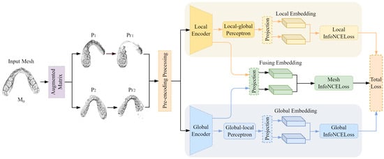
Figure 1.
The structure of the two-stream self-supervised segmentation network model with enhanced network feature representation.
3.2. Paired Feature Extraction
As the self-supervised approach in this study employs contrastive learning, it requires the construction of paired data based on the characteristics of dental data to feed into the contrastive learning framework for the extraction of high-level representational features. Accordingly, for the original data sample M0 in the unlabeled dataset, we integrate two augmentation techniques—random rotation and random translation—to generate two paired augmented matrices. The random rotation utilizes a rotational transformation expressed through axis–angle representation to derive rotation matrices. By implementing rigid-body rotation through rotation axis vector A and rotation angle T, we obtain compact 3D rotation matrices. This constructed rotation matrix formulation demonstrates enhanced adaptability for application in augmented coordinate transformations.
First, randomly generate a vector with a length of 3 and use it as rotation axis vector A. Then, convert the set initial rotation angle into rotation radians and introduce a random number as rotation angle T to make the rotation random. Finally, normalize rotation axis vector A and perform cross-multiplication and matrix exponential operations on the result after dot multiplication with rotation angle T to obtain the final rotation matrix R. The formula is as follows:
where represents the generation of a random vector of the corresponding dimension, r represents the set initial rotation angle, and I represents the unit matrix; ⊗ denotes the Kronecker product.
The two relative transformation matrices are applied to M0 to obtain the augmented samples M1 and M2. For the augmented samples, the key dental features are extracted to convert them into 24-dimensional feature matrices P1 and P2 with 10,000 meshes. The k-nearest neighbor search algorithm is used to randomly select partial meshes of the two augmented samples. In order to make the paired data similar, when the two randomly selected partial meshes are mapped back to the original sample M0, a certain number of repeated meshes should be included to form correspondence. The specific process is shown in Figure 2.
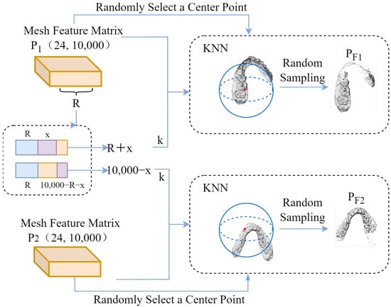
Figure 2.
Obtaining paired jaw areas.
The k-nearest neighbor search algorithm is used to obtain paired dental region features. First, according to the mesh length of the mesh feature matrix, an integer R in the range of is randomly selected as the number of meshes in the repeated mesh area in the paired samples. Based on this analysis, the mesh lengths of the paired samples are and , respectively, which are used as the numbers of meshes in the k-nearest neighbor search algorithm for the two augmented samples k. Here, x represents a random positive integer in the range of .
At the same time, a 24-dimensional feature of a mesh is randomly selected in the mesh feature matrix as the central reference eigenvalue. By calculating the Euclidean distance between the central reference eigenvalue and other mesh eigenvalues, the nearest k meshes are determined to form the dental region features, and, finally, the paired dental region features are formed. In addition, in order to normalize the paired features of the input encoder, the data length of the paired features needs to be kept consistent. To this end, 4000 mesh features are randomly sampled as paired input mesh feature data for the contrastive learning encoder.
3.3. Multi-Encoder Design
In order to enable the neural network to learn the internal common features of unlabeled data, the contrastive representation learning method is adopted, comparing different views of the same data. By calculating the similarity and differences between the data and optimizing the loss, the distance between the paired data in the feature space is shortened, and the distance between other data in the feature space is increased. Based on this, the intrinsic structure and more discriminative features of the dental data are learned. In order to effectively extract the potential feature representation of the dental mesh, PnP-3D [35] is used to improve the two-stream multi-level network [29]. The shallow and deep feature contexts are fused successively to refine the feature representation of the dental mesh, so that the self-supervised contrastive learning can more effectively extract local discriminative features and global discriminative features.
The encoder architecture of two-stream self-supervised contrastive learning is shown in Figure 3. It improves upon the two-stream semi-supervised segmentation network framework. In order to enable the self-supervised contrastive learning framework to extract the deep spatial context features of the 3D dental mesh model, inspired by PnP-3D in the representation of 3D point cloud features, PnP-3D is used to optimize the input shallow features. At the same time, the original local feature processing stream learns high-dimensional transformation residual features by stacking residual blocks, so there is a problem regarding relatively singular feature types. Based on PnP-3D, the local encoder is improved to capture the local dependencies between meshes and the global features between channels, forming spatial complementarity with the local residual features and fine-tuning and optimizing the local features to ensure that they have stronger representation capabilities. In addition, in order to better utilize the feature information at different levels, the features of different network levels in the encoder are densely connected to strengthen the synergistic relationship between the representation features.
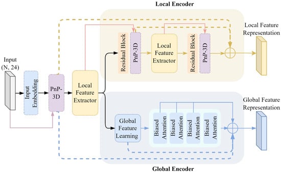
Figure 3.
Comparative learning encoder.
3.3.1. Embedded Feature Modeling
For the output of the input embedding network, PnP-3D is used to model its feature geometric relationship. The embedded feature geometric relationship modeling process is shown in Figure 4. Herein, Conv1D refers to 1D convolution, BN denotes batch normalization, ReLU and Mish are activation functions, and MLP stands for multi-layer perceptron. The inherent 3D geometric information is deeply integrated with the embedded feature , while capturing the shape characteristics of the teeth and the spatial position relationship of a single tooth in the dental model to enhance the expressiveness of the feature. PnP-3D mainly includes two parts: local context fusion and global bilinear regularization. For the original input of the entire encoder, the mesh center point coordinate is , which is first used as the coordinate guide for local context fusion. The input feature is processed by the input embedding network as the embedded feature to enhance the abstractness and expressiveness of the original feature, which helps PnP-3D to learn the geometric structure of the dental mesh data. The entire PnP-3D processing process is recorded as , and the geometric perception feature can be obtained as follows:
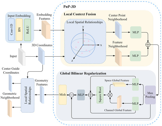
Figure 4.
Modeling process of embedding feature geometric relations.
In addition, in order to enable the encoder to fully capture the neighborhood features of the dental mesh, the local features are embedded in the original mesh feature modeling. After the embedded feature geometric relationship modeling, KNN is used to extract the mesh neighborhood features of all mesh center points. This allows the network to not only encode the single mesh features of the dental model but also process the mesh features of its surrounding areas. The local features of the dental mesh model are used as input features for the global encoder and the local encoder to capture refined local mesh feature information. The geometric perception feature and the 3D coordinates C of the original mesh center point are used as the input of the local feature extractor. The local spatial relationship modeling is shown in Figure 4, and the center-guided coordinates and its corresponding geometric neighborhood are obtained as follows:
where the number of points of the center guide coordinate and the original mesh center point C is the same, and corresponds one by one to the geometric neighborhood in the feature space to form a guide correspondence relationship.
3.3.2. Local Encoder
By introducing PnP-3D to improve the residual block, the local geometric spatial relationship of the point cloud is better captured, which compensates for the shortcomings of the stacked residual block in 3D mesh geometry modeling and enhances the geometric perception ability of the encoder. It then generates more discriminative local features and enhances the characterization ability of contrastive learning on local mesh features.
The local feature processing flow in the two-stream self-supervised encoder architecture is designed through the PnP-3D improved residual block. The PnP-3D improved residual block process in the local encoder is shown in Figure 5. Here, the residual block only uses two residual stackings. For the geometric neighborhood output by embedding geometric feature relationship modeling, the local subtle changes in the geometric neighborhood features are captured through continuous residual transformation. The improved residual design avoids information loss while improving the discrimination ability for local features. The entire residual processing process is briefly expressed as
where is the ith residual feature; represents i consecutive convolution operations, each of which is a 1-dimensional convolution; and the convolution is followed by batch normalization and a ReLU activation function. In particular, for the residual connection operation, the activation function is processed after the feature connection.
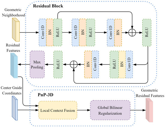
Figure 5.
PnP-3D improved residual block.
The two residual features are obtained after the output of the PnP-3D improved residual block, and the center-guided coordinates are output by the embedded geometric feature relationship modeling. PnP-3D is used for residual feature geometric modeling to obtain the geometric residual feature :
where the two residual features contain detailed information about the local area of the mesh, while the center-guided coordinates can provide a global reference for residual geometric feature modeling. Fusing the two through PnP-3D enables us to combine low-level 3D geometric features with high-level residual semantic features to obtain higher-quality feature representations. At the same time, it can enhance the model’s perception of the 3D geometric structure of the mesh and improve the discrimination of local features.
For geometric residual features and center-guided coordinates , as with the output feature processing in PnP-3D in Figure 4, local spatial relationship modeling is used as a local feature extractor to obtain the residual mesh-guided coordinates and geometric residual feature neighborhood :
The entire PnP-3D improved residual block operation is recorded as . For the residual mesh-guided coordinate and the geometric residual feature neighborhood , geometric feature perception modeling is performed to obtain the deep geometric residual feature :
In order to enable the local encoder to generate more discriminative representation features, the geometric feature models at different levels are connected to fuse the semantic feature representations at different levels. Based on this, the multi-level connection feature of the local encoder is expressed as
3.3.3. Global Encoder
For the construction of the global encoder, the network architecture setting in [28] is referenced, which consists of a global feature learning network and a multi-scale bias attention mechanism. The entire global encoder models the geometric neighborhood as a whole. Here, the global feature learning network is extracted by a simple residual transformation, which fuses the shallow local information and the deep semantic features and then abstracts the initial global information to obtain the initial global embedding information :
where is maximum pooling, through which the residual extraction features are transformed to obtain a simple global abstraction and then processed by the MLP to obtain global embedding information.
For the geometric perception feature , the output of the global feature extraction network , and the output feature of the multi-layer bias attention , a multi-level feature connection is used as the representation feature of the global encoder:
3.4. Supervised Fine-Tuning Framework
The contrastive learning pre-training framework needs to be further fine-tuned on downstream tasks to adapt to the task requirements of 3D dental model segmentation. Here, 20% of the labeled data are used for supervised fine-tuning, and the fine-tuning network framework is shown in Figure 6. Unlike the self-supervised encoder, the network input data are 24-dimensional dental features of 10,000 meshes at the labeled level. Downsampling processing is set before the two local feature processors, with 2500 meshes sampled in the first and 625 meshes sampled in the second. At the same time, an upsampling operation is set at the end of the local feature processing stream and after the dual-stream feature splicing, feature propagation is used to restore the resolution of the previous level, and a shallow residual network is used after feature propagation for propagation feature learning.
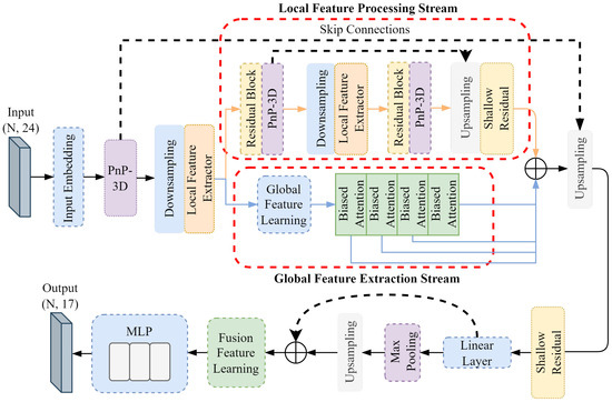
Figure 6.
Fine-tuning network framework.
The pre-trained weights of the self-supervised encoder are used as the initialization weights of the entire fine-tuning network. Since the self-supervised contrastive learning encoder has learned common discriminant features, the use of pre-trained weights can enable the encoder of the fine-tuning network to extract common dental features. This helps the fine-tuning network to converge quickly and achieve better results within a limited number of training rounds.
4. Experiments
4.1. Dataset Construction and Processing
The self-built malformation dataset is derived from real clinical cases, and high-precision intraoral scanners are used for data collection. It contains 620 hemimaxillary malformation models, covering seven major types of deformities: wisdom teeth, tooth dislocation, tooth loss, incomplete eruption, abnormal tooth spacing, crowded dentition, and implant residue. This dataset not only has rich clinical diversity but also has detailed classification and annotation information for some major deformity categories; thus, it can provide a high-quality data foundation for subsequent deep learning model training and evaluation.
In total, 80% of the severe deformity data and mild-to-moderate deformity data in the malformation dataset, representing a total of 495 mouths, are taken as the self-supervised dataset, and 20% of each, representing a total of 125 mouths, are taken as the fine-tuning dataset; meanwhile, data for a total of 925 mouths are enlarged for supervised fine-tuning.
In order to prevent the algorithm from having class imbalance problems on severe deformation data, and to enhance the generalization performance of the algorithm on severe deformation data, the supervised data are augmented in different proportions according to the deformity classification. The mild-and-moderate deformation data are augmented at a ratio of 1:5, and the severe deformation data are augmented at a ratio of 1:10. The data augmentation technique used randomly combines translation, rotation, and scaling as follows.
(1) Random translation: Random translation along the X, Y, and Z axes, with a length range of [−10, 10];
(2) Random rotation: Random rotation along the X, Y, and Z axes, with an angle range of [−180, 180];
(3) Random scaling: Random scaling along the X, Y, and Z axes, with a ratio range of [0.8, 1.0];
(4) Randomly deletion of 1% of the triangular meshes in a single model during training.
4.2. Comparative Experiment
The hardware environment of the experiment is as follows: NVIDIA GeForce RTX 3090 (The manufacturer of the NVIDIA GeForce RTX 3090 is NVIDIA, whose headquarters is located in Santa Clara, CA, USA), 24 GB memory. The software environment is as follows: Windows 10 64-bit version, Python 3.8, Pytorch 1.10.0, cuda 11.3.
The experimental training parameters are set as follows: the training cycle of the self-supervised pre-training encoder is 100 epochs, and the batch size is 4; the loss function of the self-supervised fitting optimization is PointNCELoss, the optimizer is Adam, the learning rate is 0.001, and the learning rate is adaptively adjusted by the Reduce LR On Plateau method based on the validation set loss. The training cycle of supervised fine-tuning is 200 epochs, and the loss function of fitting optimization is the Generalized Dice Loss (GDL). Other parameters are consistent with those in self-supervised pre-training.
4.2.1. Quantitative Comparison
In order to evaluate the performance of the proposed MECSegNet, comparative experiments were carried out on a self-built malformation dataset. In addition to comparing it with the self-supervised method of dental segmentation, the proposed MECSegNet was also compared with other point cloud segmentation algorithms and methods dedicated to segmenting dental models under full supervision. Therefore, all comparative experiments were divided into two parts: full supervision and self-supervision. The results are shown in Table 1.

Table 1.
Comparative experimental results.
The comparison algorithms selected in the fully supervised experiment include PointNet, PointNet++, PointMLP, PCT, MeshSegNet, MBESegNet, and MGFLNet. The proposed MECSegNet is also compared with the fully supervised experimental setting. All comparison experimental parameters are the same as the parameters of the proposed MECSegNet in the supervised fine-tuning part.
The method selected for the self-supervised experiment is the self-supervised method used for 3D dental models in [26,29], and its hyperparameter configuration is consistent with that in our self-supervised experiments.
As shown in Table 1, the proposed MECSegNet has superior performance under full supervision. Compared with PointNet, PointNet++, PointMLP, PCT, MeshSegNet, MBESegNet, and MGFLNet, the proposed MECSegNet achieves 5.61%, 13.89%, 2.25%, 3.62%, 10.13%, 29.14%, and 22.58% improvements in OA, respectively, and 12.97%, 32.16%, 5.10%, 10.65%, 19.68%, 51.87%, and 32.46% improvements in the mIoU, respectively.
Under self-supervision, the proposed MECSegNet is compared with the method in [26], and the OA is improved by 1.30%, while the mIoU is improved by 4.19%; compared with the method in [29], the OA is improved by 5.10%, and the mIoU is improved by 12.06%. The proposed MECSegNet under self-supervision is further compared with the fully supervised algorithms PointNet, PointNet++, PCT, MeshSegNet, MBESegNet, and MGFLNet, trained on all data. The OA is improved by 4.16%, 12.44%, 2.17%, 8.68%, 27.69%, and 21.13%, respectively; the mIoU is improved by 7.45%, 26.64%, 5.03%, 14.16%, 46.35%, and 26.94%, respectively. Compared with the fully supervised algorithm PointMLP, the proposed MECSegNet improves the OA by 0.80% and reduces the mIoU by 0.42%, and it is essentially the same as PointMLP in terms of accuracy.
At the same time, the comparison of the indicators Param and FLOPs shows that the lightweight nature of MECSegNet results in better overall performance and it can achieve efficient dental model segmentation with less computing resource consumption and a smaller parameter volume. In summary, the proposed MECSegNet has advanced performance under both full supervision and self-supervision conditions.
4.2.2. Quantitative Comparison
In order to intuitively display the segmentation results of the comparative experiment through a segmentation result diagram, four cases of wisdom teeth and missing teeth in different conditions were selected from the test data for visual analysis. The visual segmentation result comparison diagram is shown in Figure 7. The deformity conditions of these four cases of dental data are introduced as follows.
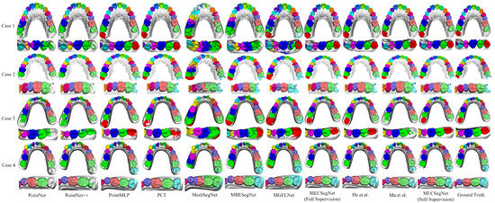
Figure 7.
Visualization of segmentation results.
Case 1: There are 14 teeth and these include the left wisdom tooth; the left first premolar is missing; and the right second molar has a residual root socket from an implant.
Case 2: There are 16 teeth; there are wisdom teeth in the bilateral half-scan state.
Case 3: A plaster scan model—there are 15 teeth, including the left wisdom tooth, and the right dentition is crowded.
Case 4: A plaster scan model—there are 14 teeth, including the right wisdom tooth; the right lateral incisor is missing; the left canine is crowded and outside the dentition; and the central incisor has a large gap.
The performance of each algorithm shown in Figure 7 on deformed dental regions is analyzed in depth, and the effect of the comparison algorithm in actual segmentation is further explained. The specific performance outcomes are as follows.
PointNet can identify large tooth gaps, but it can easily experience feature confusion in wisdom tooth data, resulting in segmentation errors in the dental model. PointNet++ has errors in the segmentation of small patches, and it can easily misidentify wisdom teeth as second molars and performs poorly on extreme deformation data. PointMLP can recognize various deformation data, but the recognition of second molar and wisdom tooth data is prone to oversegmentation to the gingival part, resulting in semantic overflow. PCT can recognize wisdom tooth data, but there are small areas of misidentification of patches in some areas, and a small number of wisdom teeth are not fully segmented.
MeshSegNet performs poorly in incisor semantics and cannot correctly identify wisdom tooth semantics. It can easily misidentify the gingival area as tooth semantics. MBESegNet has the problems of semantic confusion between teeth, unclear boundary segmentation, poor wisdom tooth recognition effects, and difficulties in dealing with various missing tooth data. The segmentation effect of MGFLNet is unstable, especially for cases with a complex gingival geometry, and it can easily segment the data into scattered and small meshes.
In contrast, the proposed MECSegNet is closest to the ground truth under full supervision, and it can still effectively identify wisdom tooth data with only 20% labeled data. Compared with the methods in [26,29], the number of mis-segmentations is very small, which demonstrates the effectiveness of the self-supervised dental model segmentation algorithm.
4.2.3. Comparison with 3DTeethSeg’22 Dataset
Comparative experiments were also conducted on the public dental model segmentation dataset 3DTeethSeg’22 to verify the robustness of the proposed algorithm on other datasets. The experimental results are shown in Table 2. Here, the dataset was pre-processed, the 3DTeethSeg’22 dataset was downsampled to 10,000 meshes, and dental models with labels mapped onto the meshes were trained and tested.
Table 2.
Comparative experimental results.
As can be seen from Table 2, the proposed MECSegNet is close to the best method, PointMLP, under full supervision and has smaller Params and FLOPs values. The proposed MECSegNet can surpass PointNet, PointNet++, MeshSegNet, MBESegNet, the method in [26], and the method in [29] under self-supervision using only 20% supervised data. Among them, the OA is improved by 1.56%, 4.11%, 2.54%, 6.95%, 0.37%, and 0.50%, respectively; the mIoU is improved by 4.38%, 9.58%, 5.33%, 16.54%, 0.70%, and 1.10%, respectively. It is close to the effects of PointMLP and PCT, with only 1.15% and 0.38% reductions in OA and 2.80% and 0.33% reductions in the mIoU. At the same time, it is essentially the same as MGFLNet, with a 0.11% improvement in OA and a 0.18% reduction in the mIoU.
4.3. Ablation Experiment
4.3.1. Effectiveness of Self-Supervised Contrastive Learning Pre-Training
In order to evaluate the importance of self-supervised pre-training in improving the overall performance of the algorithm, an ablation experiment is performed. The self-supervised contrastive learning pre-training part of the algorithm is removed, and only the supervised fine-tuning part is retained. The network is trained based on only 20% of the labeled supervised data to analyze the performance of the algorithm when supervised fine-tuning is performed on only labeled data.
The supervised fine-tuning network with only 20% labeled data was compared with the original self-supervised complete algorithm by ablation, and the convergence comparison of the training loss is shown in Figure 8. Compared with the network without self-supervision, the proposed method converges faster and has a lower final loss value.
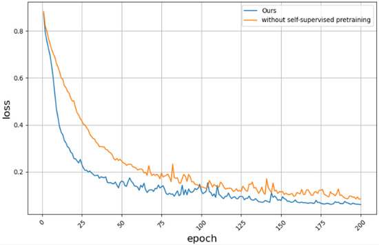
Figure 8.
Is there a loss convergence plot for self-Supervised contrastive learning pre-training.
The segmentation results of the self-supervised ablation experiment are shown in Table 3. The proposed method has 3.02% and 7.61% higher values for the OA and mIoU than the supervised fine-tuning network with only 20% labeled data, respectively, which fully demonstrates the effectiveness of the proposed self-supervised contrastive learning. Through contrastive learning pre-training, the proposed method can show stronger adaptability on unseen data. This shows that self-supervised contrastive learning pre-training can enable the model to learn common feature representations in a large amount of unlabeled data to enrich the model’s knowledge reserves. It enables it to more accurately extract features and identify common features when facing new data, thereby improving the overall performance of the algorithm in segmentation tasks.
Table 3.
Segmentation results with and without self-supervised contrastive learning pre-training.
4.3.2. Effectiveness of the Improved Network Model
In order to analyze the actual effect of the improved network model, the proposed MECSegNet is compared with the network model of reference [29] under self-supervision. The two-stream network of reference [29] is pre-trained on its encoder by self-supervised comparative learning, and supervised fine-tuning is performed on the two-stream network using 20% labeled data to test the improvement effect of the model under limited labeled data, reflecting the optimization effect of the improved algorithm on model performance. The experimental results are shown in Table 4.
Table 4.
Segmentation results with and without self-supervised contrastive learning pre-training.
As can be seen from Table 4, the proposed MECSegNet improves the OA and mIoU by 3.89% and 9.36%, respectively, compared with the two-stream algorithm before improvement. This shows the effectiveness of the improved network in the self-supervised encoder and supervised fine-tuning part. By improving the three-dimensional spatial feature representation of the mesh through PnP-3D, the generalization performance of the self-supervised segmentation algorithm on limited labeled data can be effectively improved.
4.3.3. Effectiveness of Feature Encoding of Each Part of Contrastive Learning
In order to verify the effectiveness of each part of the encoding in the pre-trained encoder of self-supervised contrastive learning, ablation experiments were performed on each feature encoding and cross-stream encoding part in the pre-trained encoder. We removes the local encoding, global encoding, and cross-stream encoding in the pre-training for loss optimization. The encoder is pre-trained by combining the encoding of each part, and the pre-trained parameters are used for supervised fine-tuning. The experimental results are shown in Table 5.
Table 5.
Segmentation results of self-supervised learning with and without local feature encoder.
Structure 1 only includes local feature encoding. The proposed method has 0.81% and 2.86% greater segmentation effects in terms of the OA and mIoU than only local feature encoding in self-supervised learning. This shows the effectiveness of global feature encoding and cross-stream feature encoding in the pre-training of self-supervised contrastive learning. It can fully learn the global universal features of the dental mesh, which helps to enhance the semantic recognition of tooth positions in the dental model.
Structure 2 includes only global feature encoding, and the proposed method has 1.00% and 3.14% greater segmentation effects in terms of the OA and mIoU, respectively, than the global feature encoder in self-supervised learning. This shows the importance of local feature encoding and cross-stream feature encoding in the pre-training of self-supervised contrastive learning, enabling the model to fully learn the local universal features of the dental mesh and helping to improve the local effect of the segmentation task.
Structure 3 is cross-stream contrast ablation, and the proposed method has 0.58% and 2.23% greater segmentation effects in terms of the OA and mIoU, respectively, than self-supervised learning without cross-stream feature encoding. This shows that cross-stream feature comparison in the pre-trained network of self-supervised contrastive learning can assist in feature alignment between global features and local features.
5. Conclusions
This paper proposes a self-supervised dental model segmentation method based on multiple encoding contrastive learning. The encoder is pre-trained by self-supervised contrastive learning to improve the generalization of deep learning methods in the dental model segmentation task. By introducing the self-supervised contrastive learning framework, the two-stream encoder is designed using embedded feature geometric relationship modeling and the PnP-3D improved residual block to extract dental augmented pair features. Then, the encoder is pre-trained via the triple loss of local features, global features, and cross-stream features to learn the universal features of the dental mesh model from multiple angles. The experimental results show that the self-supervised dental segmentation method with the improved two-stream encoder design can achieve better training results on limited labeled data.
However, for small triangular areas in crowded dentition, the algorithm is prone to identifying them as the semantics of a nearby tooth, resulting in the incorrect recognition of the gingival mesh of the triangular area. Meanwhile, the proposed method should be integrated into the orthodontic workflow via algorithmic interfaces, and scanner variability should be addressed through data standardization in the pre-processing stage. In the future, we will continue to study the small-sample dental segmentation method for triangular areas and establish an adaptive post-processing optimization process to dynamically adjust the segmentation results according to the geometric and topological characteristics of the triangular area to reduce the probability of misidentification.
Author Contributions
Conceptualization, T.M. and J.Z.; methodology, T.M., J.Z. and X.W.; software, X.W. and J.Z.; validation, X.W. and J.Z.; formal analysis, J.Z. and X.W.; resources, X.W., J.Z. and Z.Z.; data curation, X.W., J.Z. and Y.L. (Yawen Li); writing—original draft preparation, X.W. and J.Z.; writing—review and editing, X.W.; visualization, J.Z., Z.Z. and Y.L. (Yawen Li); supervision, T.M. and J.Z.; funding acquisition, T.M. and Y.L. (Yuancheng Li). All authors have read and agreed to the published version of the manuscript.
Funding
This work was supported by the National Key R&D Program of China (No. 2022ZD0119005) and in part by the Shaanxi Natural Science Fundamental Research Program Project (No. 2022JM-508).
Institutional Review Board Statement
Not applicable.
Informed Consent Statement
Not applicable.
Data Availability Statement
The datasets analyzed in the paper are sourced from the 3DTeethSeg’22 dataset: https://github.com/abenhamadou/3DTeethSeg22_challenge.
Conflicts of Interest
The authors declare no conflicts of interest.
References
- Chen, D.; Zhu, M.; Qiao, Y.; Wang, J.; Zhang, X. An ergonomic design method of manned cabin driven by human operation performance. Adv. Des. Res. 2023, 1, 2949–7825. [Google Scholar] [CrossRef]
- Ma, T.; Dang, Z.; Yang, Y.; Yang, J.; Li, J. Dental panoramic X-ray image segmentation for multi-feature coordinate position learning. Digit. Health 2024, 10, 20552076241277154. [Google Scholar] [CrossRef] [PubMed]
- Ma, T.; Zeng, Y.; Pei, W.; Li, C.; Li, Y. Tooth position prediction method based on adaptive geometry optimization. PLoS ONE 2025, 20, e0327498. [Google Scholar] [CrossRef] [PubMed]
- Ma, X.; Qin, C.; You, H.; Ran, H.; Fu, Y. Rethinking Network Design and Local Geometry in Point Cloud: A Simple Residual MLP Framework. arXiv 2022, arXiv:2202.07123. [Google Scholar] [CrossRef]
- Ma, T.; Wei, X.; Zhai, J.; Zhang, Z.; Li, Y.; Li, Y. Feature-guided multilayer encoding–decoding network for segmentation for 3D intraoral scan data. Sci. Rep. 2025, 15, 32129. [Google Scholar] [CrossRef]
- Jana, A.; Subhash, H.M.; Metaxas, D. 3D tooth mesh segmentation with simplified mesh cell representation. In Proceedings of the 2023 IEEE 20th International Symposium on Biomedical Imaging (ISBI), Cartagena, Colombia, 18–21 April 2023; IEEE: Piscataway, NJ, USA, 2023; pp. 1–5. [Google Scholar]
- Lian, C.; Wang, L.; Wu, T.H.; Wang, F.; Yap, P.T.; Ko, C.C.; Shen, D. Deep Multi-Scale Mesh Feature Learning for Automated Labeling of Raw Dental Surfaces from 3D Intraoral Scanners. IEEE Trans. Med. Imaging 2020, 39, 2440–2450. [Google Scholar] [CrossRef] [PubMed]
- Ma, T.; Li, J.; Dang, Z.; Li, Y.; Li, Y. A Dual-Stream Dental Panoramic X-Ray Image Segmentation Method Based on Transformer Heterogeneous Feature Complementation. Technologies 2025, 13, 293. [Google Scholar] [CrossRef]
- Qi, C.R.; Su, H.; Mo, K.; Guibas, L.J. Pointnet: Deep learning on point sets for 3D classification and segmentation. In Proceedings of the IEEE Conference on Computer Vision and Pattern Recognition, Honolulu, HI, USA, 21–26 July 2017; pp. 652–660. [Google Scholar]
- Qi, C.R.; Yi, L.; Su, H.; Guibas, L.J. PointNet++: Deep Hierarchical Feature Learning on Point Sets in a Metric Space. Adv. Neural Inf. Process. Syst. 2017, 30, 5105–5114. [Google Scholar]
- Li, Y.; Bu, R.; Sun, M.; Wu, W.; Di, X.; Chen, B. PointCNN: Convolution on X-Transformed Points. Adv. Neural Inf. Process. Syst. 2018, 31, 828–838. [Google Scholar]
- Xu, M.; Ding, R.; Zhao, H.; Qi, X. Paconv: Position adaptive convolution with dynamic kernel assembling on point clouds. In Proceedings of the IEEE/CVF Conference on Computer Vision and Pattern Recognition, Nashville, TN, USA, 20–25 June 2021; pp. 3173–3182. [Google Scholar]
- Hu, Q.; Yang, B.; Xie, L.; Rosa, S.; Guo, Y.; Wang, Z.; Trigoni, N.; Markham, A. Randla-net: Efficient semantic segmentation of large-scale point clouds. In Proceedings of the IEEE/CVF Conference on Computer Vision and Pattern Recognition, Seattle, WA, USA, 13–19 June 2020; pp. 11108–11117. [Google Scholar]
- Guo, M.H.; Cai, J.X.; Liu, Z.N.; Mu, T.J.; Martin, R.R.; Hu, S.-M. PCT: Point Cloud Transformer. Comput. Vis. Media 2021, 7, 187–199. [Google Scholar] [CrossRef]
- Vaswani, A.; Shazeer, N.; Parmar, N.; Uszkoreit, J.; Jones, L.; Gomez, A.N.; Kaiser, Ł.; Polosukhin, I. Attention Is All You Need. Adv. Neural Inf. Process. Syst. 2017, 30, 6000–6010. [Google Scholar]
- Xu, X.; Liu, C.; Zheng, Y. 3D Tooth Segmentation and Labeling Using Deep Convolutional Neural Networks. IEEE Trans. Vis. Comput. Graph. 2018, 25, 2336–2348. [Google Scholar] [CrossRef] [PubMed]
- Feng, Y.; Feng, Y.; You, H.; Zhao, X.; Gao, Y. Meshnet: Mesh neural network for 3D shape representation. In Proceedings of the AAAI Conference on Artificial Intelligence, Honolulu, HI, USA, 27 January–1 February 2019; Volume 33, pp. 8279–8286. [Google Scholar]
- Schult, J.; Engelmann, F.; Kontogianni, T.; Leibe, B. Dualconvmesh-net: Joint geodesic and euclidean convolutions on 3D meshes. In Proceedings of the IEEE/CVF Conference on Computer Vision and Pattern Recognition, Seattle, WA, USA, 13–19 June 2020; pp. 8612–8622. [Google Scholar]
- Zhao, Y.; Zhang, L.M.; Yang, C.S.; Tan, Y.; Liu, Y.; Li, P.; Huang, T.; Gao, C. 3D Dental Model Segmentation with Graph Attentional Convolution Network. Pattern Recognit. Lett. 2021, 152, 79–85. [Google Scholar] [CrossRef]
- Xiong, H.; Li, K.; Tan, K.; Feng, Y.; Zhou, J.T.; Hao, J.; Liu, Z. TFormer: 3D Tooth Segmentation in Mesh Scans with Geometry Guided Transformer. arXiv 2022, arXiv:2210.16627. [Google Scholar] [CrossRef]
- Li, Z.; Liu, T.; Wang, J.; Zhang, C.; Jia, X. Multi-Scale Bidirectional Enhancement Network for 3D Dental Model Segmentation. IEEE Trans. Med. Imaging 2022, 42, 467–480. [Google Scholar]
- Ma, T.; Yang, Y.; Zhai, J.; Yang, J.; Zhang, J. A tooth segmentation method based on multiple geometric feature learning. Healthcare 2022, 10, 2089. [Google Scholar] [CrossRef]
- Ben-Hamadou, A.; Smaoui, O.; Chaabouni-Chouayakh, H.; Rekik, A.; Pujades, S.; Boyer, E.; Strippoli, J.; Thollot, A.; Setbon, H.; Trosset, C.; et al. Teeth3DS: A Benchmark for Teeth Segmentation and Labeling from Intra-Oral 3D Scans. arXiv 2022, arXiv:2210.06094. [Google Scholar]
- Alsheghri, A.; Ghadiri, F.; Zhang, Y.; Lessard, O.; Keren, J.; Cheriet, F.; Guibault, F. Semi-Supervised Segmentation of Tooth from 3D Scanned Dental Arches. In Medical Imaging 2022: Image Processing; SPIE: Bellingham, WA, USA, 2022; Volume 12032, pp. 766–771. [Google Scholar]
- Liu, R.; Zhang, H. Segmentation of 3D Meshes through Spectral Clustering. In Proceedings of the 12th Pacific Conference on Computer Graphics and Applications (PG 2004), Seoul, Republic of Korea, 6–8 October 2004; IEEE: Piscataway, NJ, USA, 2004; pp. 298–305. [Google Scholar]
- He, X.; Wang, H.; Hu, H.; Yang, J.; Feng, Y.; Wang, G.; Zuozhu, L. Unsupervised Pre-Training Improves Tooth Segmentation in 3-Dimensional Intraoral Mesh Scans. In Proceedings of the International Conference on Medical Imaging with Deep Learning, Virtual, 6–8 July 2022; pp. 493–507. [Google Scholar]
- Wang, Y.; Sun, Y.; Liu, Z.; Sarma, S.E.; Bronstein, M.M.; Solomon, J.M. Dynamic graph cnn for learning on point clouds. ACM Trans. Graph. (TOG) 2019, 38, 146. [Google Scholar] [CrossRef]
- Liu, Z.; He, X.; Wang, H.; Xiong, H.; Zhang, Y.; Wang, G.; Hao, J.; Feng, Y.; Zhu, F.; Hu, H. Hierarchical self-supervised learning for 3D tooth segmentation in intra-oral mesh scans. IEEE Trans. Med Imaging 2022, 42, 467–480. [Google Scholar] [CrossRef] [PubMed]
- Ma, T.; Zhai, J.; Wei, X.; Leng, Y.; Li, Y. Semi-Supervised Learning-Based Dual-Stream Multi-Hierarchical Semantic Segmentation Method for Malocclusion Models. J.-Comput.-Aided Des. Comput. Graph. 2025, 1–12. [Google Scholar] [CrossRef]
- Zhang, Z.; Yang, B.; Wang, B.; Li, B. GrowSP: Unsupervised Semantic Segmentation of 3D Point Clouds. In Proceedings of the IEEE/CVF Conference on Computer Vision and Pattern Recognition, Vancouver, BC, Canada, 17–24 June 2023; IEEE: Piscataway, NJ, USA, 2023; pp. 17619–17629. [Google Scholar]
- Hu, Q.; Yang, B.; Fang, G.; Guo, Y.; Leonardis, A.; Trigoni, N.; Markham, A. SQN: Weakly-Supervised Semantic Segmentation of Large-Scale 3D Point Clouds. In Proceedings of the European Conference on Computer Vision, Tel Aviv, Israel, 23–27 October 2022; Springer: Cham, Switzerland, 2022; pp. 600–619. [Google Scholar]
- Pang, Y.; Wang, W.; Tay, F.E.H.; Liu, W.; Tian, Y.; Yuan, L. Masked Autoencoders for Point Cloud Self-Supervised Learning. In Proceedings of the European Conference on Computer Vision, Tel Aviv, Israel, 23–27 October 2022; Springer: Cham, Switzerland, 2022; pp. 604–621. [Google Scholar]
- Yu, X.; Tang, L.; Rao, Y.; Huang, T.; Zhou, J.; Lu, J. Point-BERT: Pre-Training 3D Point Cloud Transformers with Masked Point Modeling. In Proceedings of the IEEE/CVF Conference on Computer Vision and Pattern Recognition, New Orleans, LA, USA, 18–24 June 2022; IEEE: Piscataway, NJ, USA, 2022; pp. 19313–19322. [Google Scholar]
- Xu, X.; Lee, G.H. Weakly Supervised Semantic Point Cloud Segmentation: Towards 10x Fewer Labels. In Proceedings of the IEEE/CVF Conference on Computer Vision and Pattern Recognition, Seattle, WA, USA, 13–19 June 2020; IEEE: Piscataway, NJ, USA, 2020; pp. 13706–13715. [Google Scholar]
- Qiu, S.; Anwar, S.; Barnes, N. PnP-3D: A Plug-and-Play for 3D Point Clouds. IEEE Trans. Pattern Anal. Mach. Intell. 2021, 45, 1312–1319. [Google Scholar] [CrossRef]
Disclaimer/Publisher’s Note: The statements, opinions and data contained in all publications are solely those of the individual author(s) and contributor(s) and not of MDPI and/or the editor(s). MDPI and/or the editor(s) disclaim responsibility for any injury to people or property resulting from any ideas, methods, instructions or products referred to in the content. |
© 2025 by the authors. Licensee MDPI, Basel, Switzerland. This article is an open access article distributed under the terms and conditions of the Creative Commons Attribution (CC BY) license (https://creativecommons.org/licenses/by/4.0/).