Abstract
Lane-changing maneuvers critically influence traffic flow and safety. This study introduces the Global Optimal Lane-Changing (GOLC) model, a framework that optimizes decisions by quantitatively predicting their systemic effects on surrounding traffic. Unlike traditional models that focus on immediate neighbors, the GOLC model integrates a kinematic wave model to precisely quantify the spatiotemporal impacts on the entire affected platoon, striking a balance between local vehicle actions and global traffic efficiency. Implemented in the Simulation of Urban Mobility (SUMO) environment, the GOLC model is evaluated against benchmark models Minimizing Overall Braking Induced by Lane Changes (MOBIL) and SUMO LC2013. Comparative evaluations demonstrate the GOLC model’s superior performance. In a three-lane scenario, the GOLC model significantly enhances traffic efficiency, reducing average delay by 3.4% to 46.8% compared to MOBIL under medium- to high-flow conditions. It also fosters a safer environment by reducing unnecessary lane changes by 1.1 times compared to the LC2013 model. In incident scenarios, the GOLC model shows greater adaptability, achieving higher average speeds and lower travel times while minimizing speed dispersion and deceleration. These findings validate the effectiveness of embedding macroscopic traffic theory into microscopic driving decisions. The model’s unique strength lies in its ability to predict and minimize the collective negative impact on all affected vehicles, representing a significant step towards real-world implementation in Advanced Driver-Assistance Systems (ADAS) and enhancing safety in next-generation intelligent transportation systems.
1. Introduction
The rapid development of Advanced Driver-Assistance Systems (ADAS) has opened new avenues for enhancing road capacity through precise control over the movements of individual vehicles. Lane-changing behavior, being a fundamental aspect of lateral vehicle motion, plays a critical role in this process. However, such uncoordinated maneuvers often have unintended consequences, adversely affecting surrounding vehicles and contributing to disturbances that can degrade the operational efficiency of the entire road network [1]. To address this challenge, it is essential to leverage the perception and computational capabilities of modern ADAS technologies, enabling a more accurate and rational prediction of the impact of lane-changing decisions on the surrounding traffic environment. By integrating these predictions into the lane-changing decision-making process, it becomes possible to optimize vehicle actions, potentially improving overall traffic flow and safety.
When making lane-changing decisions, most existing vehicle lane-changing models—such as the Gipps-type model, the utility theory model, and the cellular automata model—typically evaluate the risks and benefits of lane-changing behavior from the perspective of the lane-changing vehicle [2]. However, these models often fail to fully account for the broader impact of lane-changing maneuvers on the surrounding traffic environment, focusing primarily on the behavior of the individual vehicle rather than considering the collective effect on the entire system. As a result, they cannot provide a global optimal lane-changing decision that minimizes the total travel time of all vehicles within the road network. A notable exception is the MOBIL (Minimizing Overall Braking Induced by Lane Changes) model, which takes into account the lane-changing vehicle and two adjacent following vehicles, one from the target lane and one from the original lane. Despite its merits, the MOBIL model assumes that only two vehicles are impacted by the lane change, which is not always the case. In fact, recent studies based on real-world data indicate that a single lane-changing maneuver typically affects 4 to 5 vehicles for a duration of approximately 12 to 20 s [3]. This limitation means that such locally optimal decisions can inadvertently trigger cascading decelerations, contributing to traffic oscillations and phantom jams. A global perspective, in contrast, anticipates this ripple effect. The practical benefits of such a forward-looking model are significant, including enhanced traffic stability, reduced unnecessary braking, lower fuel consumption, and, ultimately, improved overall road network capacity. Given this, the primary goal of this paper is to explore how to quantitatively estimate the impact of lane-changing behavior before making lane-changing decisions, and to incorporate this impact into the decision-making process to improve traffic flow optimization.
Research on the impact of lane-changing behavior can be broadly classified into two categories: the effects of mandatory lane changes in specific road sections (such as at freeway ramps, incident sites, and signalized intersections), and the effects of discretionary lane changes in other general road sections. Gong and Du [4] utilized traffic flow theory to explore the spatial interaction mechanism of multiple lane changes and proposed a method for calculating the optimal lane-change prompt point near exit ramps. Mehr and Eskandarian [5] proposed an innovative sentinel system for intelligent vehicles to enhance traffic safety and efficiency after freeway incidents. Similarly, Fu et al. [6] developed a cellular automaton (CA) model to study the complex lane-changing behaviors of left-turning vehicles in contraflow lane designs at signalized intersections. Xiao et al. [7] also explored discretionary lane-changing on multi-lane curved roads using lattice hydrodynamic models, analyzing traffic stability to explain the formation of bottlenecks. Chen and Ahn [8] applied traffic flow theory to study the spatial disruptions caused by the limited acceleration of vehicles during multiple lane changes. Tian et al. [9] proposed a two-lane lattice model to investigate the synergistic effects of drivers’ desire for smooth driving and aggressive lane-changing behaviors on traffic stability.
Limited research efforts have employed vehicle-trajectory data to explore the specific impacts of lane-changing behavior on discrete aspects of transportation systems, particularly focusing on traffic safety, operational efficiency, and energy consumption. He et al. [3] introduced a novel approach based on real vehicle-trajectory data to study the impact of a single discretionary lane-changing behavior on surrounding traffic. Their analysis of high-precision Zen-traffic data revealed that, on average, a lane change affects 4 to 5 vehicles for a duration of 12 to 13 s. Chen et al. [10] developed a proactive risk-level prediction method for lane-changing behavior, enabling the estimation of collision risk before the lane-changing vehicle completes the maneuver. Wang et al. [11] used Next Generation Simulation (NGSIM) trajectory data to confirm the important influence of driving habits on traffic efficiency during lane-changing process. Yan et al. [12] developed an ecological evaluation framework for analyzing lane-changing behaviors, through which they identified the variation trend in accelerator pedal depth as a critical determinant influencing vehicular fuel consumption. Yan et al. [13] reviewed the research on lane-changing duration and its influencing factors.
Research on lane-changing decision-making model can be categorized into rule-based lane-changing models, utility-based lane-changing models, and artificial intelligence-based lane-changing models [2]. Kesting et al. [14] introduced the MOBIL model, which incorporates both safety criteria and incentive criteria. According to this model, a lane change occurs only when the expected acceleration of adjacent rear vehicle in the target lane exceeds a minimum threshold, and the total acceleration change of three vehicles involved—the lane-changing vehicle and two adjacent rear vehicles (one from the target lane and one from the original lane)—exceeds a predefined threshold. Li et al. [15] developed a lane-changing model for connected and automated vehicles based on safety potential field theory. It analyzed the distribution of safety potential fields for the relevant vehicles and derived the minimum safety distance required during the lane-changing process. Chen et al. [16] proposed three lane-changing control strategies for merge bottlenecks, demonstrating that connected and automated vehicle can enhance overall traffic system performance. Xie et al. [17] developed a data-driven lane-changing model based on deep learning, which utilized deep belief networks for decision-making and long short-term memory neural networks for lane-changing execution. The model was trained and tested using NGSIM data. Gao et al. [18] proposed a multi-intelligent vehicle lane-changing method using deep reinforcement learning. Compared with other methods, the new method can improve average vehicle speed and mitigate traffic congestion. Yang et al. [19] proposed a deep reinforcement learning algorithm that integrates an LSTM trajectory prediction model to enhance the safety and efficiency of lane-changing decisions. To address the challenge of collaboration in multi-agent scenarios, Bi et al. [20] proposed a Mix Q-learning method for collaborative lane-changing decisions, which coordinates individual and global Q networks to balance individual and collective benefits.
Some researchers use game theory to study drivers’ lane-changing decisions [21,22,23,24,25,26]. Ali et al. [21] combined target lane selection using the utility theory approach with gap acceptance behavior modeled by game theory to create a comprehensive lane-changing decision framework. The results indicated that the novel framework could handle failed lane-changing scenarios, making it well-suited for connected driving traffic environments and capable of more accurately simulating real lane-changing decisions. Guo and Harmati [22] viewed the lane-changing process as a non-zero-sum, non-cooperative game among multiple agents, with the goal of maximizing lane capacity. A new decomposition algorithm based on game theory was proposed to improve computational efficiency. Simulations demonstrated that, under congested traffic conditions, this approach outperformed rule-based methods in therms of lane-changing decision-making. Yao and Du [23] also employed a game-theoretic framework to examine lane-changing behaviors in the vicinity of bus bay stops. Their findings underscored the significance of bus drivers’ driving styles in elucidating the interactions between passenger vehicles and bus drivers’ behaviors. Ji and Levinson, Ji et al. [24,25] developed two-player non-cooperative lane-changing game framework to study interactions between lane-changing vehicle and the following vehicle in the target lane. The simulation results demonstrated the new method can reduce aggressive lane changes in congested traffic. To address the challenges of generalization in complex scenarios, Yang et al. [26] proposed a hybrid model that combines game theory with deep reinforcement learning (DRL), using the DRL agent to adaptively adjust the game-theoretic payoff function to enhance safety and efficiency.
Researchers have increasingly incorporated trajectory planning components into lane-changing decision models, recognizing the importance of path optimization in the lane-changing process [27,28,29,30,31]. Huang et al. [27] proposed a novel approach for lane-changing control using improved random trees to generate trajectory clusters. They applied fuzzy linguistic preference relations to identify driver preferences, enabling personalized trajectory planning and lane-change control. Jin et al. [28] employed quintic polynomials for lane-changing trajectory planning and a tracking error model for lateral and longitudinal controllers, demonstrating enhanced tracking performance. Sun et al. [29] considered the motion control of the lane-changing vehicle, the vehicle on the target lane, and the following vehicles on the original lane into upper-layer and lower-layer, and established a multi-objective optimization framework to design a smooth lane-changing trajectory. Xiong et al. [30] proposed a trajectory planning algorithm that incorporates a predictive model to estimate the number of vehicles affected by a lane change, thereby minimizing its impact. Zhang et al. [31] developed an integrated learning model that recognizes driver lane-changing intention in a connected environment, finding that connectivity significantly increases the prediction time window. Similarly, Jing et al. [32] utilized deep reinforcement learning as a decision model to directly plan efficient and eco-friendly lane-changing trajectories, demonstrating significant reductions in both fuel consumption and maneuver completion time.
Although the existing literature has made significant advances, several key challenges remain. Utility-based models like MOBIL, while foundational, are limited by their local perspective; AI-based models, though powerful, often lack interpretability, posing challenges for safety verification; and other paradigms frequently rely on simplifying assumptions, such as perfect driver rationality. A common, unresolved challenge across these approaches is the difficulty of quantitatively predicting the global impact of a lane-changing maneuver before it occurs and subsequently incorporating this systemic impact into the decision-making process. To address this gap, this paper first relaxes the assumption in the MOBIL model, which considers only two following vehicles, by utilizing the kinematic wave model from traffic flow theory and vehicle-following characteristics. This approach predicts the number of vehicles affected by lane-changing behavior and models the motion transition changes of all the impacted following vehicles. Subsequently, the paper develops a secondary module in the SUMO simulation software via the Traffic Control Interface (TraCI) interface to simulate the newly proposed global optimal lane-changing model. The main contributions of this paper are as follows:
- A novel Global Optimal Lane-Changing (GOLC) model is proposed that fully accounts for the systemic impact of lane changes on all affected vehicles. The model’s effectiveness is demonstrated by simulation results, which show that in the tested scenarios, it in particular, decreases the average delay by 3.4% to 46.8% compared to the MOBIL model under medium- to high-flow conditions and reduces the average number of lane changes by 1.1 times relative to LC2013 under low- to medium-flow conditions.This model provides a ‘globally optimal’ decision at the platoon level, aiming to minimize unnecessary lane-changing maneuvers by considering the entire traffic wave generated by the action, which is a significant expansion over models that only consider immediate neighbors.
- The performance of the proposed model is rigorously evaluated through a comparative analysis with established benchmarks (MOBIL and LC2013), which validates its advantages: (1) the new proposed global optimal lane-changing model outperforms the MOBIL model in certain traffic efficiency and safety metrics; (2) the new model demonstrates superior performance over the LC2013 model in terms of specific traffic safety indicators. Furthermore, in the context of the broader literature that includes complex ‘black-box’ AI models, a key contribution of our GOLC model is its transparent, ‘white-box’ decision logic, which is derived from interpretable traffic flow principles and offers a clear advantage for safety verification.
The rest of the paper is organized as follows. Section 2 introduces the MOBIL lane-changing model and Intelligent Driver Model (IDM) car-following model, presents the proposed global optimal lane-changing model, and analyses the number of vehicles impacted by lane-changing behavior. Section 3 outlines the simulation method for implementing the global lane-changing model and discusses the traffic simulation scenarios, evaluation indicators and simulation parameters. Section 4 presents a comparative analysis of the simulation results for three lane-changing models: the MOBIL model, LC2013 model, and the global optimal lane-changing model. Section 5 discusses the findings, including the model’s assumptions, limitations, and a roadmap for real-world implementation. Finally, Section 6 concludes the work.
2. Methodology
This section details the formulation of the proposed Global Optimal Lane-Changing (GOLC) model. In Section 2.1, we review the foundational models upon which our work is built—the MOBIL lane-changing model and the IDM car-following model. In Section 2.2, we introduce our primary contribution, the GOLC model, which extends the MOBIL framework. Finally, in Section 2.3, we detail the novel method developed to quantify the number of vehicles impacted by a lane change, which is a core component of the GOLC model.
2.1. The MOBIL Lane-Changing Model and IDM Car-Following Model
The MOBIL lane-changing model, proposed by Kesting et al. [14], evaluates a lane change based on the vehicles involved, as illustrated in Figure 1. This includes the self-vehicle (SV), its leading vehicle (LV) and following vehicle () in the original lane, and the target-lane leading vehicle (TLV) and target-lane following vehicle (). The model is designed to minimize the braking induced by the lane change on the SV, , and . This model incorporates two key criteria: the safety criteria and incentive criteria. The safety criterion stipulates that when the self-vehicle enters target lane, the acceleration of the adjacent rear vehicle in the target lane must exceed a safety threshold (in m/s2). In other words, the deceleration of vehicle cannot be smaller than the safety limit:
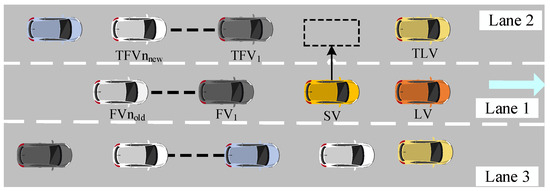
Figure 1.
Schematic diagram of lane-changing behavior.
The incentive criterion stipulates that when the self-vehicle enters target lane instantaneously, the acceleration changes of the self-vehicle () and two immediately following vehicles (,) must exceed a given threshold (in m/s2). In other words, the acceleration gain generated by lane-changing should be greater than a certain value:
where p is the politeness factor, which represents the extent to which the driver considers the acceleration gains of two adjacent vehicles in both lanes during the lane-change process. The value of p ranges from 0 to 1, with a larger value indicating that the driver gives more consideration to the acceleration gains of the adjacent vehicles.
Since the predicted accelerations () used in the MOBIL lane-changing model cannot be directly obtained, they needs to be estimated using a car-following model. In this paper, the commonly used IDM is employed to predict these parameters. The IDM, proposed by [33], considers that vehicle acceleration is influenced by several factors, including maximum acceleration (in m/s2), vehicle speed v (in m/s), free flow speed (in m/s), acceleration index (dimensionless), desired vehicle spacing (in m), vehicle spacing s (in m), speed difference (in m/s), stationary safety distance (in m), safe time headway T (in s), and vehicle comfortable deceleration b (in m/s2). The specific calculation formula is as follows:
2.2. The Global Optimal Lane-Changing Model
Building upon the incentive criterion of the MOBIL model, this section introduces our primary contribution: the GOLC model. When the vehicle in front suddenly decelerates or accelerates while driving, the self-vehicle will most likely adjust its speed to maintain safety and traffic efficiency. In the lane-changing decision model, the MOBIL model only accounts for the acceleration changes of the self-vehicle and the adjacent following vehicles, but it does not fully capture the broader impact of lane-changing behavior on surrounding traffic. In other words, the model should consider all vehicles affected by the lane change, not just those ‘immediately’ adjacent vehicles. Let the number of affected vehicles in the original lane and the target lane be denoted as and , respectively. This means the model considers the entire platoon of following vehicles in both the original lane (from to ) and the target lane (from to ), extending the scenario shown in Figure 1. Consequently, Equation (2) should be rewritten as Equation (5). The method for determining and will be shown in the next section.
where and represent the accelerations of the i-th and j-th following vehicles in the original lane and the target lane, respectively, after the vehicle moves to the target lane. Similar to the MOBIL lane-changing model, and can be easily calculated using the car-following model, assuming the self-vehicle instantaneously moves into the target lane and the space gaps of and change suddenly. However, since the space gaps of – and – do not changed instantaneously, their accelerations would not be directly affected according to the car-following model’s calculations. Therefore, alternative methods need to be employed to calculate their accelerations. The change in vehicle acceleration is caused by lane-changing is assumed to follow a decreasing acceleration pattern, where the vehicles – and – imitate the acceleration-change pattern of the preceding vehicle, as described by the following equation:
To better illustrate the core contribution of our work, Figure 2 provides a side-by-side comparison of the incentive logic, contrasting the local perspective of models like MOBIL with the global perspective of the GOLC model. The key distinction lies in the scope of impact assessment. While MOBIL considers a fixed set of three vehicles, the GOLC model first dynamically quantifies the number of all affected vehicles before evaluating the systemic impact on the entire platoon.
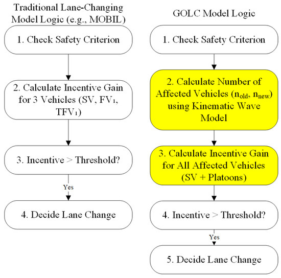
Figure 2.
Comparison of local and global lane-changing models. The highlighted step represents the core contribution of the GOLC model.
2.3. The Number of Vehicles Impacted by Lane-Changing Behavior
A core component of the GOLC model is the ability to quantify the number of impacted vehicles ( and ); this section presents the novel method developed for this purpose. This paper employs traffic flow theory to analyze the number of vehicles impacted by lane-changing, assuming that the fluctuations in acceleration caused by lane-changing generate traffic waves. Before the lane-changing wave is generated, vehicles travel on road section at an average speed (in m/s), with a traffic density of (in veh/m) and a traffic flow of (in veh/s). After the lane-changing wave is generated, the wave propagates at the speed of (in m/s), and the speed of vehicles passing through the traffic wave surface is , with a traffic density of and a traffic flow of . If the lane-changing wave lasts for a duration of (in s), the number of vehicles passing through the traffic wave surface can be calculated as follows:
This equation involves . The vehicle’s speed before lane-changing can be easily obtained, the traffic flow before lane-changing can be calculated using the classic speed-density relationship, such as Green-shields equation, as shown in Equation (10).
where is the jam density (in veh/m). The lane-changing wave duration can be interpreted as the lane-changing impact time. A recent study on lane-changing impacts, based on actual data, reveals that the lane-changing impact time is influenced by various factors, such as driver attributes and traffic scenes, leading to significant fluctuations and making accurate estimation challenging. Therefore, this paper adopts the average lane-changing impact time of 12.5 s, obtained from previous studies ([3,34]), as the value of . Furthermore, the range of is expanded to 5–20 s.
The last parameter in Equation (9) is the wave speed . By substituting the basic relationship of traffic flow q, density k, and speed v (), along with the density-speed relationship (Equation (10)), into the wave speed calculation equation, we can derive the relationship between wave speed and vehicle’s speeds, as shown in Equation (11).
When the traffic flow is in a balanced state, meaning that the vehicles are moving at a constant speed, the relationship between space gap and vehicle’s speed can be calculated by the IDM model (Equation (3)), assuming that .
The traffic flow is in a balanced state before lane-changing, after the lane-changing effect dissipates, the traffic flow returns to a balanced state. During this process, the space gap between vehicles can be assumed to become times the original value. The vehicle’s average acceleration during this period can be obtained by adjusting the acceleration calculated using Equations (3) and (13), taking into the account the change in space gap. It is assumed that the average acceleration during this period is adjusted by a factor of , where is a dimensionless deceleration-reduction coefficient representing the ratio of instantaneous to average deceleration. The corresponding calculation equation is shown in Equation (14). Then the speed of the vehicle can then be determined. Finally, by substituting Equation (15) into Equation (11) and combining it with Equation (8), Equation (16) can be derived, which allows for calculation of the number of vehicles affected by lane-changing. Although Equation (16) appears complicated, it only requires real-time collection of vehicle speed data, other parameters are hyper-parameters that are solely dependent on road conditions.
From Equation (16), it can be observed that the longer lane-changing impact time is, the more vehicles are affected. Similarly, the closer the vehicle speed is to the free-flow speed , the more vehicles are impacted. To better illustrate the influences of and on the number of impacted vehicles, these two parameters are discretized, while other hyper-parameters are set to , , , , , or 2. The number of vehicles impacted by lane-changing is calculated using Equation (16), and the results are shown in Figure 3. As the number of vehicles in target (original) lane increases (decreases), the space gap-change coefficient for target (original) lane is set to 0.5 (2). As shown in Figure 3, the number of affected vehicles in the target lane is greater than that in the original lane. Additionally, when lane-changing impact time is set to be greater than 15 s, the number of affected vehicles tends be overestimated. The acceleration correction parameter can be determined through simulation experiments.
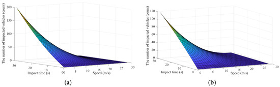
Figure 3.
The number of vehicles impacted by lane-changing in different lanes. (a) Impact in the target lane. (b) Impact in the original lane.
3. Simulations
This paper utilizes the TraCI interface to perform secondary development of the SUMO simulation software (version 1.22.0), enabling the simulation of the newly proposed lane-changing model, namely the Global Optimal Lane-Changing (GOLC) model.
3.1. The Traffic Scene and Simulation Flowchart
The purpose of this simulation is to evaluate the advantages and disadvantages of the proposed lane-changing model. To eliminate the influence of special road segments, a simple two-way, six-lane straight road is selected as the traffic scenario, featuring a maximum speed limit of 100 km/h, lane widths of 3.75 m, and a total length of 2 km. Two distinct driving scenarios are simulated on this segment: (i) a baseline scenario reflecting standard, unobstructed traffic flow; and (ii) an incident scenario in which an accident-induced obstruction blocks the middle lane. The benchmark lane-changing models used for comparison are the LC 2013 model provided by SUMO and the MOBIL lane-changing model. Since the MOBIL and the GOLC models cannot be used directly implemented in the SUMO simulation software, this paper employs Python (version 3.12) programming to construct both models and utilizes the TraCI interface to enable communication between SUMO and Python.
The simulation flowchart of the GOLC model is shown in in Figure 4. Given that the GOLC model exhibits a higher degree of complexity compared to the MOBIL model, the latter can be derived through the elimination of specific procedural steps from the former. Consequently, the flowchart illustrating the MOBIL simulation has been intentionally omitted from this presentation. The primary code used to implement both models consists of the following steps: (1) Analyze all vehicles in the traffic scenario to identify the self-vehicle’s leading and following vehicles in both the self-lane and adjacent lanes, and gather the relevant parameters; (2) Calculate the safety criteria using Equation (1), then determine the number of impacted vehicles using Equation (16), and calculate the incentive criteria using by using Equation (8); (3) Determine whether to change lanes and the direction of the lane change (left or right). Lane-changing occurs only when both safety and incentive criteria are met. The direction of lane change (left or right) is based on the magnitude of the lane-changing benefits, which is the left-hand term of Equation (8). Additionally, if there are no following vehicles for self-vehicle, the acceleration parameters of following vehicles are set to 0. If there are no leading vehicles for the self-vehicle, the speed parameters of the leading vehicles are set to the maximum speed limit, the gap between the leading vehicle and self-vehicle is set to infinity.
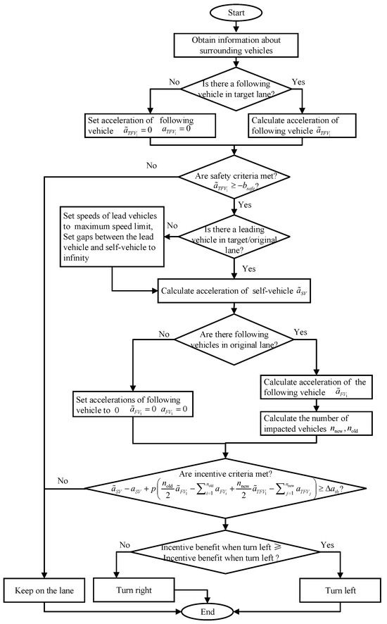
Figure 4.
The simulation flowchart of the GOLC model.
3.2. Evaluation Indicators
This paper uses several indicators, including the number of lane changes, vehicle travel time, delay time, speed dispersion, and vehicle deceleration, to evaluate and compare the performance of different lane-changing models.
Frequent discretionary lane changes can reduce driving comfort, increase risks, and prolong travel time. Therefore, the total or average number of lane changes all vehicles throughout the simulation can serve as an indicator of the lane-changing model’s quality. Generally speaking, under identical conditions, a lane-changing model with fewer lane-changes is considered superior.
The purpose of discretionary lane change is to achieve a better driving environment. Key indicators, such as average travel time () (in s), average delay time () (in s), and the proportion of average delay to average travel time () (dimensionless), are essential for assessing the rationality of lance-changing decisions and evaluating the impact of different lane-changing models on traffic efficiency. The smaller the values of these indicators, the better the lane-changing model employed.
where and are the actual travel time and the expected travel time (in s) of the i-th vehicle, respectively. n is the total number of vehicles in the simulation process.
Vehicle speed dispersion is a key measure of the traffic disturbance caused by lane-changing behavior [35]. The speed standard deviation, 85th percentile vehicle speed, and 15th percentile vehicle speed are selected as indicators to assess the degree of vehicle speed dispersion. The speed standard deviation describes the deviation of each vehicle’s speed from the average speed of all vehicles. The 85th and 15th percentiles speed are commonly used as benchmarks for determining the maximum and minimum allowable speed on roads. These indicators serve as important references for traffic safety indicators. The smaller the speed standard deviation, the smaller the disturbance caused by lane-changing, and the safer the traffic environment.
The lane-changing model should aim to minimize the braking behavior of surrounding vehicles. Frequent braking not only increases the travel time but also lead to higher fuel consumption and greater traffic emissions. Therefore, the paper uses the number of braking vehicles and the total deceleration of all vehicles as indicators to evaluate the performance of different lane-changing models.
3.3. Parameter Settings
Except for the deceleration-reduction coefficient , all other hyper-parameters have been given in the model introduction part. represents the ration of instantaneous deceleration to average deceleration, and it is a value greater than 1. All other parameters are kept constant, and is varied from 2 to 10. Simulations are conducted, and the average travel time and number of lane changes are used as evaluation indicators to determine the optimal value of .
The simulation results are shown in Table 1. When or 6, the average travel time and number of lane changes are at their smallest, and either value can be selected. However, since yields better results than , is chosen. It is worth noting that although the difference in average travel time is small for different values of , considering the large number of vehicles, the difference still has certain significance. For completeness, the other parameters are set as follows: , , or 2, , , , , , .

Table 1.
Simulation results under different deceleration-reduction coefficients when input flow is 4500 veh/h.
To analyze the impact of different lane-changing models on various vehicle-movement indicators under different traffic flow conditions, this paper sets the initial traffic flow range to [500–5000 veh/h] at intervals. This range was deliberately chosen to cover key traffic states, from free-flow to congested conditions. The interval was deemed sufficient to capture the performance trends of the different models as traffic density increases, striking a balance between granular detail and computational efficiency. Therefore, the selected set is representative and sufficient for the study’s primary objective of conducting a fundamental comparative analysis. Each simulation lasts for , with a time step of , a standard value in microscopic traffic simulation that provides sufficient temporal resolution to accurately capture vehicle dynamics without excessive computational cost.
4. Results Analysis
This section presents a comparative analysis of the simulation results for the GOLC, MOBIL [14], and LC2013 models across the scenarios and parameters detailed in the previous section. The performance of each model is evaluated based on key metrics for traffic efficiency and safety. The analysis begins with Scenario (i), the baseline case representing standard, unobstructed traffic flow.
4.1. Spatiotemporal Trajectory
The space-time trajectory diagram for different lane-changing models at a traffic volume of 4500 veh/h is shown in in Figure 5. As seen from Figure 5a,c, both LC2013 and GOLC lane-changing models produce favorable results. Except for the initial stage, vehicles maintain high-speed operation. However, Figure 5b demonstrates that traffic flow using MOBIL lane-changing model exhibits significant traffic fluctuations between 500–700 s and 500–1200 m. This indicates that the newly proposed GOLC model perfroms better than MOBIL model.
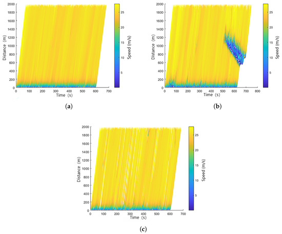
Figure 5.
The space-time trajectory diagram for different lane-changing models when traffic volume is 4500 veh/h. (a) LC2013 model. (b) MOBIL model. (c) GOLC model.
4.2. The Number of Lane Changes
The simulation results for the total number of lane changes and the average number of lane change, as generated by different lane-changing models, are presented in Figure 6. As illustrated in Figure 6, both the total and average number of lane changes initially increase and then decrease with increasing traffic flow. For the MOBIL lane-changing model, both metrics peak at approximately 4500 veh/h. For the GOLC model, the peak occurs at around 4000 veh/h. In contrast, for the LC2013 model, the largest number of lane changes occurs at a traffic flow of about 2600 veh/h, while the maximum average number of lane changes is observed at around 1000 veh/h. With the exception of extremely high traffic flows exceeding 4800 veh/h, the GOLC model consistently generates fewer lane changes and a lower average number of lane changes than the MOBIL model across almost all traffic flow levels. This indicates that the GOLC model is more effective at minimizing lane changes. For traffic flows below approximately 3700 veh/h, both the total and average number of lane changes generated by GOLC model are lower than those of the LC2013 model. When the traffic volume is less than 2500 veh/h, the LC2013 model results in significantly more lane changes than the GOLC model. In the simulated three-lane road scenario spanning 2 km, with traffic volumes ranging from 500 to 3500 vehicles per hour, the GOLC model generated an average of 1.1 fewer lane changes per vehicle compared to the LC2013 model. These findings suggest that under low- and medium-traffic flow conditions, the GOLC model is more efficient by reducing what it considers to be unnecessary lane changes generated by the LC2013 model.
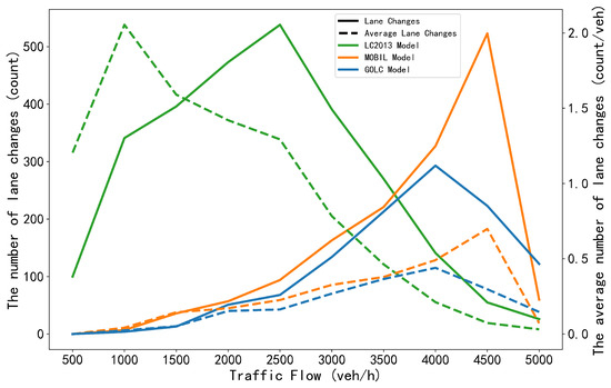
Figure 6.
The lane-change numbers under different traffic volumes for different LC models in scenario (i).
4.3. The Average Travel Time and the Average Delay Time
The average travel time and average delay time for different lane-changing models under varying traffic volumes are presented in Figure 7. As illustrated in the figure, within the traffic flow range of 3500 to 5000 veh/h, the MOBIL model exhibits significantly higher average travel times and delays compared to the other two models under investigation. Specifically, in this traffic regime, the GOLC model demonstrates a notable reduction in delay, achieving an average decrease of 25.11% relative to the MOBIL model. This indicates that by relaxing the assumption in the MOBIL model, where only two following vehicles are considered, and by incorporating the impact of multiple following vehicles as done in the GOLC model, traffic delays can be significantly reduced, leading to improved traffic efficiency.
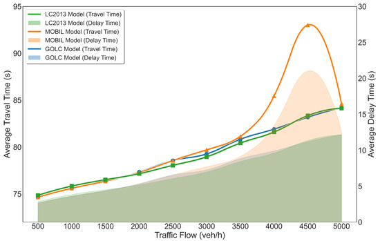
Figure 7.
The average travel time and average delay time under different traffic volumes for different LC models in scenario (i).
4.4. Traffic Safety Analysis
The standard deviation of speed and the violin chart of vehicle speeds under different traffic volumes for different lane-changing models are shown in Figure 8 and Figure 9. When the traffic flow ranges from 500 to 3500 veh/h, the speed standard deviations generated by the three lane-changing models are similar. However, when the traffic flow is between 4000 and 4500 veh/h, the speed standard deviation generated by the MOBIL lane-changing model is significantly higher than that of the GOLC or LC2013 model. A large standard deviation of vehicle speeds indicates greater speed dispersion, which increases driving risks and is detrimental to traffic safety. Figure 9 further illustrates this point, as the violin plot (Figure 9b) for the MOBIL model shows a noticeable tailing phenomenon, confirming the large dispersion in vehicle speeds. This suggests that under high traffic flow conditions, the lane-changing behavior generated by the GOLC model can help reduce traffic risks compared to the MOBIL model.
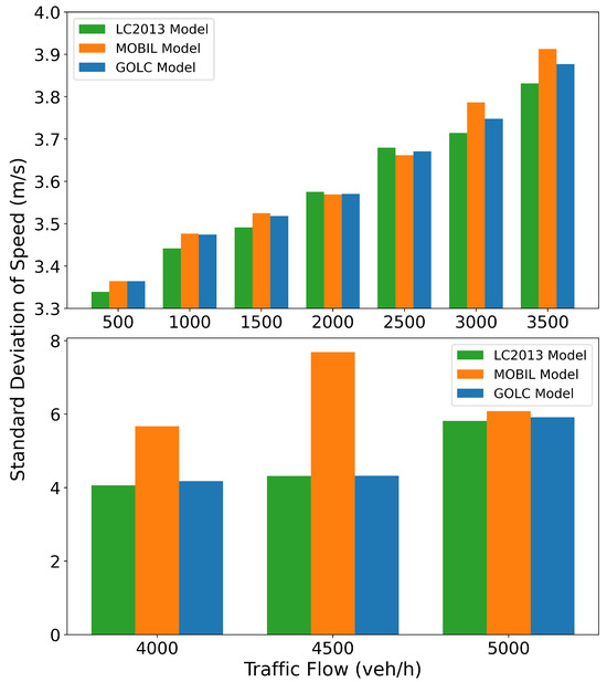
Figure 8.
The standard deviation of speed under different traffic volumes for different LC models in scenario (i).
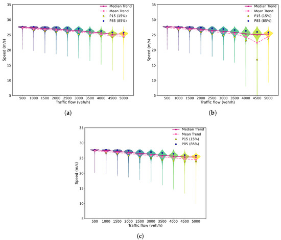
Figure 9.
The violin chart of vehicle speeds under different traffic volumes for different LC models in scenario (i). (a) LC2013 model. (b) MOBIL model. (c) GOLC model.
Total deceleration quantifies the cumulative magnitude of braking events. A lower value indicates smoother traffic flow and enhanced safety. The total decelerations of all vehicles and the number of breaking vehicles under different traffic volume for different lane-changing models are shown in Figure 10 and Figure 11. When the traffic flow is between 500 and 2500 veh/h, the total decelerations of all vehicles generated by three lane-changing models are relatively small. However, when the traffic flow is between 3000 and 4500 veh/h, the total deceleration generated by the MOBIL lane-changing model is significantly higher than that of the GOLC model. Despite this, the number of braking vehicles generated by both models within this traffic flow range is comparable, suggesting that the lane-changing behavior induced by the MOBIL model results in a higher average deceleration compared to the GOLC model. When traffic flow reaches 5000 veh/h, the total decelerations generated by all three lane-changing models are similar. This indicates that in terms of the total deceleration caused by lane-changing, the GOLC model performs significantly better than the MOBIL model in medium- and high-traffic scenarios, while the effects of the three lane-changing models are nearly identical in other scenarios. When the traffic flow is between 500 and 3500 veh/h, the number of braking vehicles generated by the LC2013 model is higher than that of the GOLC model. In other traffic scenarios, the number of braking vehicles generated by all three lane-changing models is similar. This indicates that, under low and medium-traffic flow conditions, the lane-changing behavior generated by the GOLC model affects fewer vehicles and performs better than the LC2013 model.
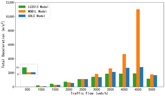
Figure 10.
All the vehicles’ total decelerations under different traffic volume for different LC models in scenario (i).
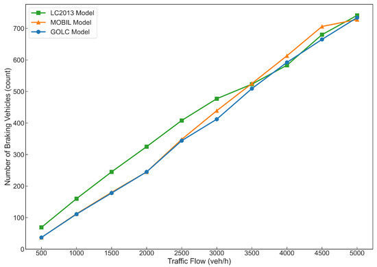
Figure 11.
The number of braking vehicles under different traffic volume for different LC models in scenario (i).
Complementing Scenario (i), to analyze the impact of different lane-changing models on various vehicle-movement indicators under disrupted traffic flow conditions, this paper sets the initial traffic flow range in Scenario (ii) to [1000–5000 veh/h] at 1000 veh/h intervals. At 300 s into the simulation, a traffic incident occurs in the 800–1200 m segment, rendering the middle lane impassable. In the incident scenario, the MOBIL model and the GOLC model exhibit an abnormally high rate of lane-change operations in the SUMO environment. To enhance simulation fidelity, a lane-change cooldown interval is introduced for each model. Based on the results of multiple simulation experiments, the configuration yielding optimal performance is selected, with cooldown durations of 15 s at flow rates of 1000, 2000, and 3000 veh/h, 30 s at 4000 veh/h, and 25 s at 5000 veh/h.
4.5. Travel Efficiency
In the incident scenario, different lane-changing models exhibit a significant increase in lane-change frequency as evidenced by Figure 12, since vehicles are required to perform additional maneuvers to mitigate the accident’s impact on travel efficiency. For flows between 1000 to 3000 veh/h, both the GOLC model and the MOBIL model generate more lane changes than the LC2013 model. As flow increases, the GOLC model’s frequency falls below that of the LC2013 model beyond 4400 veh/h. While the MOBIL model’s count, though reduced, remains higher than the GOLC model’s. However, lane-change frequency alone is an insufficient metric for evaluating model effectiveness in incident scenarios, as such events inherently compel vehicles to perform additional maneuvers. Therefore, average travel time and delay time are analyzed in Figure 13.
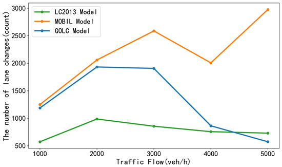
Figure 12.
The lane-change numbers under different traffic volumes for different LC models in scenario (ii).
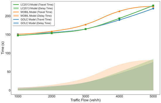
Figure 13.
The average travel time and average delay time under different traffic volumes for different LC models in scenario (ii).
As shown in Figure 13, for flows from 1000 to 3000 veh/h, the LC2013 model yields the shortest travel times and lowest delays. As flow increases, the GOLC model surpasses the LC2013 model at 3000 veh/h and subsequently records the best performance up to 5000 veh/h. The MOBIL model consistently produces the longest travel times and greatest delays. These results suggest that the GOLC model’s adaptive strategy effectively reduces travel time in medium to high flows. In contrast, the LC2013 model’s conservative behavior limits its performance, and the MOBIL model’s high maneuver rate fails to produce corresponding time savings, increasing its performance deficit. In summary, the GOLC model shows superior adaptability to accident-induced disruptions, outperforming both the MOBIL model and the LC2013 model in overall travel efficiency under medium- to high-flow conditions, while the MOBIL model’s suitability remains limited.
4.6. Traffic Safety
To evaluate the safety performance of the different models under the incident scenario, key traffic state parameters including average speed, speed standard deviation, and total deceleration were analyzed across a range of traffic flows.
The relationships between traffic flow and average speed in Figure 14 and between traffic flow and speed stability in Figure 15 reveal critical differences between the models. While the average speed for all models decreases as flow increases, their performance characteristics diverge significantly. In the 1000 to 3000 veh/h range, the GOLC model’s average speed is slightly lower than the LC2013 model’s, but this gap progressively narrows. As flow surpasses 3000 veh/h, the GOLC model’s average speed overtakes that of the LC2013 model. This is complemented by its superior stability; the GOLC model maintains a consistently low-speed standard deviation at medium to high flows. In contrast, the LC2013 model, while starting with the lowest standard deviation at 1000 veh/h, becomes increasingly unstable at higher flows, with its speed deviation eventually exceeding that of the generally poor-performing MOBIL model. The MOBIL model consistently exhibits the lowest average speed and a high speed standard deviation, indicating poor performance in both efficiency and safety.
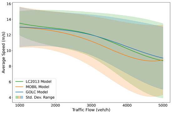
Figure 14.
The average speed under different traffic volumes for different LC models in scenario (ii).
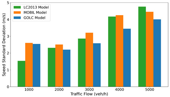
Figure 15.
The standard deviation of speed under different traffic volumes for different LC models in scenario (ii).
The analysis of total deceleration presented in Figure 16 reveals even more pronounced differences. The value for the MOBIL model escalates dramatically in medium- and high-traffic scenarios, becoming significantly higher than that of the GOLC and LC2013 models. Whereas the LC2013 model yields lower total deceleration than the GOLC model at flows of 1000 to 3000 veh/h, the GOLC model registers the lower total deceleration at 4000 veh/h. This indicates that while the LC2013 model is more effective at minimizing deceleration in lower-density traffic, the GOLC model’s strategy becomes more advantageous for maintaining smooth flow under very high-density conditions.
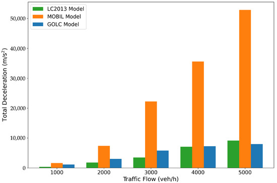
Figure 16.
All the vehicles’ total decelerations under different traffic volume for different LC models in scenario (ii).
4.7. On the Interpretation of ‘Global Optimal’
The term ‘global optimal,’ as used in this paper’s title and contributions, warrants clarification to avoid ambiguity. In the strict sense of control theory and optimization, a global optimum refers to a solution that is superior to all other feasible solutions across the entire problem space and time horizon. Our model does not claim to achieve global optimality in this network-wide, long-term context.
Instead, ‘global optimal’ is used here to describe the scope of the decision-making process for a single maneuver. It signifies that the GOLC model’s decision is optimal for the entire affected platoon of vehicles, in contrast to traditional models like MOBIL, which are only locally optimal as they consider just a few immediate vehicles. This claim of systemic superiority is not merely theoretical; it is directly supported by our simulation results in Section 4. The significant reductions in average delay, speed dispersion, and total deceleration observed when using the GOLC model—especially compared to the locally optimal MOBIL model in high-flow and incident scenarios—provide empirical evidence that optimizing for the entire platoon yields demonstrably superior outcomes at a systemic, albeit localized, level. Therefore, while not globally optimal in the network-wide sense, the GOLC model represents a critical step from local optimization towards a more holistic, system-level approach, which we refer to as being ‘globally optimal at the platoon level.’
5. Discussion
The simulation results presented in this study demonstrate the theoretical advantages of the GOLC model in enhancing traffic efficiency and safety compared to established benchmarks. However, the transition from a simulated environment to real-world application presents several challenges and limitations that warrant discussion.
5.1. Model Assumptions and Real-World Data Calibration
The GOLC model’s foundation rests on the use of idealized kinematic wave equations to calculate the number of affected vehicles, which assumes a continuous and homogeneous traffic flow. This is an idealization, as real-world driver reactions are discrete, nonlinear, and influenced by a multitude of human factors such as attention, experience, and individual behavior. However, despite these abstractions, this physics-based approach provides a crucial theoretical foundation for understanding the systemic impact of lane changes and represents a significant advancement over models that consider only immediate neighbors. In reality, these variations in driving can lead to different outcomes than predicted by the idealized wave equations, meaning the model’s impact estimates may be exaggerated in some cases. To address potentially poorer performance when applied to real-world data, future work could focus on developing a hybrid model that integrates machine learning components to capture the stochastic nature of driver heterogeneity, thereby refining the impact prediction.
Similarly, the model assumes a linear distribution of acceleration change propagating through the following platoon. This is a first-order approximation, as the reaction of each driver is highly individual and may not follow a simple proportional decay. The model also relies on two key parameters, the politeness factor (‘p’) and the incentive threshold (‘’), to govern its decision-making. We acknowledge that quantifying complex human behaviors like altruism and motivation with constant parameters is a simplification. However, a theoretical analysis clarifies their critical roles. The politeness factor ‘p’ directly controls the trade-off between the subject vehicle’s gain and the disruption caused to others; a higher ‘p’ value makes the model more ‘altruistic,’ leading to fewer but more systemically beneficial lane changes. The incentive threshold ‘’ acts as a general filter, making the model more conservative by requiring a larger potential gain for any maneuver to be considered. Together, these parameters serve as powerful, interpretable levers for tuning the model’s assertiveness to match different driving styles or traffic scenarios.
Furthermore, as this study focuses on theoretical development, many parameters in the model were not obtained through direct measurement but were predefined based on benchmark values from the literature that represent standard traffic conditions. We acknowledge that in real-world applications, this could lead to errors if these parameters are not properly adjusted. A key strength of our model, however, is that many of its core parameters are directly tied to fundamental and observable traffic characteristics such as speed and density. Therefore, for any practical deployment, a rigorous calibration process using local, real-world trajectory data is essential to accurately reflect the specific driving culture and road conditions of a given area. To ground our model in reality as much as possible at this stage, we adopted a lane-changing impact time (‘’ = 12.5 s) directly from empirical studies using real-world data [3,34]. However, we acknowledge that using a constant average value is a simplification. The actual impact time is highly context-dependent, varying with traffic conditions (e.g., congestion levels) and road types (e.g., highways vs. urban streets), making a universal value difficult to establish. Our analysis in Section 2.3 (see Figure 3), which illustrates the theoretical impact of varying ‘’ on the number of affected vehicles, underscores that for practical application, this parameter must be carefully calibrated to reflect local conditions. Validating the model’s core cause-and-effect mechanisms also presents significant challenges, which is why controlled simulation serves as a critical first step.
5.2. Validation in a Simulated Environment
A significant limitation of this study is that the GOLC model has been validated exclusively within the SUMO simulation environment. While simulation allows for controlled and repeatable experiments, it does not fully capture the complexities and unpredictability of real-world traffic. For instance, factors such as imperfect sensor data from cameras or LiDAR, and communication latencies in a connected vehicle network, would introduce noise and delays into the state variables (e.g., speed, position) used by the model. Specifically, errors in vehicle state estimation would directly propagate into the car-following model calculations, leading to inaccurate predictions of accelerations. This, in turn, could cause the GOLC model to misjudge the safety and incentive criteria, potentially resulting in either overly conservative behavior (missing safe lane-changing opportunities) or overly aggressive maneuvers. Furthermore, the presence of non-standard vehicle types or vulnerable road users (pedestrians, cyclists) was not considered, as the kinematic wave theory is ill-suited to model their distinct and often erratic movement patterns.
The current study was also limited to a straight highway segment. Our results confirm that the GOLC model provides excellent performance and clear advantages in this context of uninterrupted flow. However, its applicability to more complex geometries with interrupted flow, such as merges, diverges, and urban intersections, is a considerable research challenge. In these more complex scenarios, the model’s effectiveness may be influenced by other factors, such as the prevalence of mandatory lane changes, which operate on a different logic than the benefit-driven discretionary maneuvers our model is designed for. These scenarios introduce numerous additional factors, including traffic signals, complex right-of-way rules, and interactions with turning or crossing traffic, which are not accounted for in the current formulation. For example, at an intersection, the ‘optimal’ lane-changing decision is constrained not only by traffic efficiency but also by signal timing and the presence of opposing vehicles, fundamentally altering the problem definition. Therefore, extending the GOLC model to such environments would require substantial modifications, and its direct application is currently limited. It is important to note that the high-flow conditions simulated in both our baseline and incident scenarios already produced severe congestion and stop-and-go waves. The strong performance of the GOLC model under these demanding conditions has demonstrated its effectiveness. However, the model has not been tested in conditions of complete gridlock, where traffic is at a total standstill. In such paralyzed traffic flow, the opportunities and incentives for lane-changing are minimal, and the applicability of any discretionary lane-changing model becomes inherently limited. Thus, while our model is effective in congested and stop-and-go traffic, its behavior in a completely gridlocked regime remains an open question.
Furthermore, the model’s scalability and real-time performance in large-scale, multi-agent environments require careful consideration. The computational cost of running the GOLC model is a critical factor for ADAS integration. Unlike the MOBIL model, which performs a fixed number of calculations for three key vehicles, the GOLC model’s complexity scales with the number of affected vehicles ( and ). However, it is important to note that the calculations themselves—solving algebraic equations from the IDM and kinematic wave theory—are computationally inexpensive. The primary overhead comes from iterating through the platoon. Based on our simulation environment, even in dense traffic where the platoon size might reach 10–15 vehicles, the total computation time per decision step remains on the order of milliseconds, well within the capabilities of modern automotive-grade processors. This suggests that the model is feasible for real-time ADAS integration. Nevertheless, for deployment in very large-scale, dense networks, further code optimization would be essential to guarantee real-time performance under all conditions. Additionally, while our model’s ‘global’ perspective is an advancement, it is still limited to the immediate consequences of a single maneuver. In a large multi-agent environment, it does not currently model systemic, network-wide chain reactions. Addressing these higher-level dynamics is a complex but important direction for future research.
5.3. Comparison with Other Modeling Paradigms
This paper provides a quantitative comparison against the widely used MOBIL and LC2013 models. It is also valuable to qualitatively position the GOLC model within the broader landscape of lane-changing research, particularly in relation to artificial intelligence (AI)-based approaches. AI models, such as those using deep reinforcement learning [18,32], have shown great promise in learning complex driving behaviors from large datasets. Their strength lies in their ability to capture nuanced, nonlinear interactions without relying on explicit physical formulations. However, they often function as ‘black boxes,’ making their decision-making process difficult to interpret and their safety difficult to formally verify, a challenge that has motivated the development of hybrid approaches [26].
In contrast, the GOLC model is a ‘white-box’ model. Its decisions are fully interpretable and are derived from established traffic flow principles. This transparency is a significant advantage for safety-critical applications like autonomous driving. The trade-off is a reliance on idealized assumptions, as discussed previously. We believe that physics-based models like GOLC and data-driven AI models are not mutually exclusive. A promising direction for future research is the development of hybrid models that combine the predictive power of AI with the interpretability and safety guarantees of physics-based frameworks.
5.4. Roadmap for Real-World Implementation
Bridging the gap between simulation and real-world deployment requires a phased approach. The first step is offline validation using large-scale, real-world trajectory datasets. This would allow for the calibration of model parameters and an assessment of its performance against actual human driving behavior. The subsequent phase would involve Hardware-in-the-Loop (HIL) and Vehicle-in-the-Loop (VIL) simulations, which test the model’s real-time computational performance and its interaction with physical vehicle components. The final stage would be controlled field testing on a closed track, followed by pilot programs in live traffic. This roadmap provides a clear pathway to progressively validate and refine the GOLC model, addressing any performance gaps identified at each stage, for its eventual integration into production ADAS.
6. Conclusions
This paper presents the Global Optimal Lane-Changing (GOLC) model, a novel framework that addresses the limitations of existing approaches like the MOBIL model, which consider only a few adjacent vehicles. The model’s key advantage lies in its ability to move beyond a localized perspective. By integrating kinematic wave theory, the GOLC model establishes a relationship between key traffic parameters and the number of impacted vehicles. It then models the dynamic behavior of the entire affected platoon, assuming following vehicles replicate the deceleration of the leading vehicle in a decreasing form. This allows the GOLC model to quantitatively predict and fully account for the systemic, spatiotemporal impact of a lane change, leading to decisions that are globally superior and result in a reduction in unnecessary lane changes.
Furthermore, this paper implements the GOLC model through a joint simulation framework combining SUMO and Python, and compares the performance of the GOLC model with that of the MOBIL and LC2013 models in both standard and incident-induced traffic scenarios. Through the comparison of various performance indicators—including space-time trajectory diagrams, lane changes number, vehicle travel time and delay time, speed dispersion, and vehicle deceleration—the following conclusions are drawn:
- 1.
- Traffic efficiency: In baseline traffic scenarios, the GOLC model performs comparably to the LC2013 model. Under incident scenarios, its advantages become more pronounced. The GOLC model demonstrates superior adaptability to disruptions, achieving higher average speeds and lower travel times than both the LC2013 and MOBIL models, particularly under medium- to high-flow conditions.
- 2.
- Traffic safety: The GOLC model consistently fosters a safer traffic environment. In standard scenarios, it reduces unnecessary lane changes and braking events compared to the LC2013 model under low and medium flows. In the more demanding incident scenario, it demonstrates superior safety performance across the board by simultaneously minimizing speed dispersion and reducing the magnitude of deceleration, outperforming both the LC2013 and MOBIL models.
Despite these promising results, the study has several limitations, primarily its reliance on idealized assumptions and a simulated environment, as detailed in the Discussion section. Future research will focus on the roadmap outlined, beginning with validating and calibrating the GOLC model against real-world trajectory data before extending its application to more complex traffic scenarios. Addressing these challenges is crucial for realizing the model’s full potential. Ultimately, the GOLC model provides a robust and interpretable physics-based logic that can serve as a foundational component for next-generation Advanced Driver-Assistance Systems (ADAS) and centralized traffic control strategies, contributing to the development of safer and more efficient autonomous transportation systems.
Author Contributions
Conceptualization, J.H. and Y.H.; methodology, J.H.; software, Y.H.; validation, W.Z., Z.Z., W.L. and T.W.; formal analysis, J.H. and Y.H.; investigation, W.Z.; resources, J.H.; data curation, Y.H.; writing—original draft preparation, J.H., Y.H. and Z.Z.; writing—review and editing, W.Z. and Z.Z.; visualization, Z.Z., T.W. and W.L.; supervision, J.H. and Z.Z.; project administration, J.H.; funding acquisition, J.H. All authors have read and agreed to the published version of the manuscript.
Funding
This research was funded by the National Natural Science Foundation of China, grant numbers 72371004 and 72001007.
Institutional Review Board Statement
Not applicable.
Informed Consent Statement
Not applicable.
Data Availability Statement
The data presented in this study are available on request from the corresponding author.
Conflicts of Interest
The authors declare no conflicts of interest.
References
- Di, Y.; Zhang, W.; Ding, H.; Zheng, X.; Ran, B. Cooperative control of dynamic CAV dedicated lanes and vehicle active lane-changing in expressway bottleneck areas. Phys. A Stat. Mech. Its Appl. 2024, 638, 129623. [Google Scholar] [CrossRef]
- Zheng, Z. Recent developments and research needs in modeling lane-changing. Transp. Res. Part B Methodol. 2014, 60, 16–32. [Google Scholar] [CrossRef]
- He, J.; Qu, J.; Zhang, J.; He, Z. The impact of a single discretionary lane change on surrounding traffic: An analytic investigation. IEEE Trans. Intell. Transp. Syst. 2022, 24, 554–563. [Google Scholar] [CrossRef]
- Gong, S.; Du, L. Optimal location of advance warning for mandatory lane change near a two-lane highway off-ramp. Transp. Res. Part B Methodol. 2016, 84, 1–30. [Google Scholar] [CrossRef]
- Mehr, G.; Eskandarian, A. Sentinel: An onboard lane change advisory system for intelligent vehicles to reduce traffic delay during freeway incidents. IEEE Trans. Intell. Transp. Syst. 2021, 23, 8906–8917. [Google Scholar] [CrossRef]
- Fu, D.J.; Zhang, C.B.; Liu, J.; Li, T.; Li, Q.L. Research of the left-turn vehicles lane-changing behaviors at signalized intersections with contraflow lane. Phys. A Stat. Mech. Its Appl. 2024, 633, 129364. [Google Scholar] [CrossRef]
- Xiao, Y.; Wu, W.; Zhai, C.; Zhai, M.; Zhang, J. Analysis of empirical lane-changing rate effect on multi-lane traffic on curved roads. Chin. J. Phys. 2025, 95, 260–274. [Google Scholar] [CrossRef]
- Chen, D.; Ahn, S. Capacity-drop at extended bottlenecks: Merge, diverge, and weave. Transp. Res. Part B Methodol. 2018, 108, 1–20. [Google Scholar] [CrossRef]
- Tian, C.; Yang, S.; Kang, Y. A novel two-lane lattice model considering the synergistic effects of drivers’ smooth driving and aggressive lane-changing behaviors. Symmetry 2024, 16, 1430. [Google Scholar] [CrossRef]
- Chen, T.; Shi, X.; Wong, Y.D.; Yu, X. Predicting lane-changing risk level based on vehicles’ space-series features: A pre-emptive learning approach. Transp. Res. Part C Emerg. Technol. 2020, 116, 102646. [Google Scholar] [CrossRef]
- Wang, T.; Lu, H.; Sun, Z.; Wang, J. Lane changing and keeping as mediating variables to investigate the impact of driving habits on efficiency: An EWM-GRA and CB-SEM approach with trajectory data. IET Intell. Transp. Syst. 2024, 18, 230–243. [Google Scholar] [CrossRef]
- Yan, L.; Gao, Y.; Deng, G.; Guo, J. Eco-driving strategies in lane-change behaviors use: How do drivers reduce fuel consumption? Travel Behav. Soc. 2025, 39, 100970. [Google Scholar] [CrossRef]
- Yang, F.; Liu, Q. Driver Lane-changing and Intelligent Vehicles Lane-changing Duration: State of the Art. In Proceedings of the 2024 8th CAA International Conference on Vehicular Control and Intelligence (CVCI), Chongqing, China, 25–27 October 2024; pp. 1–8. [Google Scholar]
- Kesting, A.; Treiber, M.; Helbing, D. General lane-changing model MOBIL for car-following models. Transp. Res. Rec. 2007, 1999, 86–94. [Google Scholar] [CrossRef]
- Li, L.; Gan, J.; Zhou, K.; Qu, X.; Ran, B. A novel lane-changing model of connected and automated vehicles: Using the safety potential field theory. Phys. A Stat. Mech. Its Appl. 2020, 559, 125039. [Google Scholar] [CrossRef]
- Chen, D.; Srivastava, A.; Ahn, S. Harnessing connected and automated vehicle technologies to control lane changes at freeway merge bottlenecks in mixed traffic. Transp. Res. Part C Emerg. Technol. 2021, 123, 102950. [Google Scholar] [CrossRef]
- Xie, D.F.; Fang, Z.Z.; Jia, B.; He, Z. A data-driven lane-changing model based on deep learning. Transp. Res. Part C Emerg. Technol. 2019, 106, 41–60. [Google Scholar] [CrossRef]
- Gao, H.; Zhao, M.; Zheng, X.; Wang, C.; Zhou, L.; Wang, Y.; Ma, L.; Cheng, B.; Wu, Z.; Li, Y. An improved hierarchical deep reinforcement learning algorithm for multi-intelligent vehicle lane change. Neurocomputing 2024, 609, 128482. [Google Scholar] [CrossRef]
- Yang, Z.; Wu, Z.; Wang, Y.; Wu, H. Deep Reinforcement Learning Lane-Changing Decision Algorithm for Intelligent Vehicles Combining LSTM Trajectory Prediction. World Electr. Veh. J. 2024, 15, 173. [Google Scholar] [CrossRef]
- Bi, X.; He, M.; Sun, Y. Mix Q-learning for lane-changing: A collaborative decision-making method in multi-agent deep reinforcement learning. IEEE Trans. Veh. Technol. 2025, 74, 8664–8677. [Google Scholar] [CrossRef]
- Ali, Y.; Zheng, Z.; Haque, M.M.; Yildirimoglu, M.; Washington, S. CLACD: A complete LAne-Changing decision modeling framework for the connected and traditional environments. Transp. Res. Part C Emerg. Technol. 2021, 128, 103162. [Google Scholar] [CrossRef]
- Guo, J.; Harmati, I. Lane-changing decision modelling in congested traffic with a game theory-based decomposition algorithm. Eng. Appl. Artif. Intell. 2022, 107, 104530. [Google Scholar] [CrossRef]
- Yao, R.; Du, X. Modelling lane-changing behaviors for bus exiting at bus bay stops considering driving styles: A game theoretical approach. Travel Behav. Soc. 2022, 29, 319–329. [Google Scholar] [CrossRef]
- Ji, A.; Levinson, D. Estimating the social gap with a game theory model of lane-changing. IEEE Trans. Intell. Transp. Syst. 2020, 22, 6320–6329. [Google Scholar] [CrossRef]
- Ji, A.; Ramezani, M.; Levinson, D. Pricing lane changes. Transp. Res. Part C Emerg. Technol. 2023, 149, 104062. [Google Scholar] [CrossRef]
- Yang, L.; Cao, C.; Zhao, Q.; Yang, J.; Fan, A. Lane-Changing Strategy for Autonomous Vehicle with Adaptive Adjustment of Decision-Making Preference based on Game Theory. IEEE Trans. Veh. Technol. 2025. early access. [Google Scholar] [CrossRef]
- Huang, C.; Huang, H.; Hang, P.; Gao, H.; Wu, J.; Huang, Z.; Lv, C. Personalized trajectory planning and control of lane-change maneuvers for autonomous driving. IEEE Trans. Veh. Technol. 2021, 70, 5511–5523. [Google Scholar] [CrossRef]
- Jin, M.; Qu, M.; Gao, Q.; Huang, Z.; Su, T.; Liang, Z. Advanced Trajectory Planning and Control for Autonomous Vehicles with Quintic Polynomials. Sensors 2024, 24, 7928. [Google Scholar] [CrossRef] [PubMed]
- Sun, K.; Gong, S.; Zhou, Y.; Chen, Z.; Zhao, X.; Wu, X. A multi-vehicle cooperative control scheme in mitigating traffic oscillation with smooth tracking-objective switching for a single-vehicle lane change scenario. Transp. Res. Part C Emerg. Technol. 2024, 159, 104487. [Google Scholar] [CrossRef]
- Xiong, X.; He, Y.; Cai, Y.; Liu, Q.; Wang, H.; Chen, L. A lane-changing trajectory planning algorithm based on lane-change impact prediction. IEEE Trans. Intell. Veh. 2024, 9, 7912–7930. [Google Scholar] [CrossRef]
- Zhang, H.; Gao, S.; Guo, Y. Driver lane-changing intention recognition based on stacking ensemble learning in the connected environment: A driving simulator study. IEEE Trans. Intell. Transp. Syst. 2023, 25, 1503–1518. [Google Scholar] [CrossRef]
- Jing, S.; Feng, Y.; Hui, F.; Liu, J.; Zhao, X.; Khattak, A.J. Efficient and Eco Lane-Changing Trajectory Planning for Connected and Automated Vehicles: Deep Reinforcement Learning-Based Method. IEEE Trans. Intell. Transp. Syst. 2025, 26, 9882–9892. [Google Scholar] [CrossRef]
- Treiber, M.; Hennecke, A.; Helbing, D. Congested traffic states in empirical observations and microscopic simulations. Phys. Rev. E 2000, 62, 1805. [Google Scholar] [CrossRef]
- Oh, S.; Yeo, H. Estimation of capacity drop in highway merging sections. Transp. Res. Rec. 2012, 2286, 111–121. [Google Scholar] [CrossRef]
- Shankar, V.; Mannering, F. Modeling the endogeneity of lane-mean speeds and lane-speed deviations: A structural equations approach. Transp. Res. Part A Policy Pract. 1998, 32, 311–322. [Google Scholar] [CrossRef]


Disclaimer/Publisher’s Note: The statements, opinions and data contained in all publications are solely those of the individual author(s) and contributor(s) and not of MDPI and/or the editor(s). MDPI and/or the editor(s) disclaim responsibility for any injury to people or property resulting from any ideas, methods, instructions or products referred to in the content. |
© 2025 by the authors. Licensee MDPI, Basel, Switzerland. This article is an open access article distributed under the terms and conditions of the Creative Commons Attribution (CC BY) license (https://creativecommons.org/licenses/by/4.0/).