Innovative Investigation of the Influence of a Variable Load on Unbalance Fault Diagnosis Technologies

Abstract

This paper focuses on the influence of torsional loading on the vibration-based unbalance fault diagnosis technology under variable-speed conditions. The coupled flexural–torsional nonstationary governing equations of motion are obtained and solved numerically. Taking the short-time chirp Fourier transform from the acceleration signal, which is determined from the numerical solutions, the influence of variable loading on the magnitude of the fundamental rotational harmonic—a diagnostic feature for conventional unbalance diagnosis technology—as well as its speed-invariant version for novel unbalance diagnosis technology is assessed. Numerical assessment shows that despite the stationary conditions, where the first rotational harmonic magnitude is independent from the torsional load, the conventional unbalance technology depends on the variable torsional load. However, the novel speed-invariant diagnostic technology is independent of the variable torsional load. The dependency of the conventional unbalance fault diagnosis technology on the variable torsional load and the independency of the novel speed-invariant unbalance diagnostic technology on the variable loading are justified by performing thorough experimental investigations on a variable-speed wind turbine with a permissible level of unbalance.

1. Introduction

In practice, it is not possible to have a fully balanced rotating machine [1]. So, all the rotating machines experience a permissible level of unbalance, which is not harmful for their operational conditions [1]. However, if the unbalance fault severity is increased, the level of stress coming from the fault will also be increased, which can even lead to catastrophic damage [1,2].

In view of the physical nature of the unbalance phenomenon, which is caused by the centrifugal excitation [3,4], this fault is reflected in the magnitude of the first rotational harmonic associated with the vibration signal [5,6,7,8,9,10]. Thus, the intensity of this particular frequency component is proportional to the machine rotational speed [11]. This speed dependency is the main signature that distinguishes the mass unbalance fault from other types of load-related faults [12].

Puerto-Santana et al. [13] assessed the unbalance fault diagnosis in a general disc–shaft-bearing system operating at multiple constant rotational speeds. Regarding the dependency of the fundamental rotational harmonic intensity on the operational speed, they indicated that the diagnostic system should be calibrated at different levels of the rotational speed. Furthermore, diagnosis must be carried out in no-load conditions. Notably, this study did not cover non-stationary conditions.

Ewert et al. [14] diagnosed an unbalance fault in a servo-drive system that includes two rotors with elastic interconnections and operates under variable rotational speeds. They processed vibration data using short-time Fourier transform and diagnosed the fault by monitoring the magnitude of the frequency component that coincides with the fundamental rotational harmonic. This investigation was performed in no-active load conditions, and the results were reported only for one constant operational speed.

According to reference [2], around 20% of wind turbines are operating under unbalanced conditions caused by blade imperfections, which may occur during the manufacturing, transportation, or installation processes [15] or during the operational conditions due to icing [16,17] or erosion [18,19]. These make wind turbines one of the most vulnerable rotating machines to the unbalance fault [20], whose health conditions need to be continuously monitored in order to avoid high maintenance costs [21].

Ramlau and Niebsch [22] adopted the finite element method to assess the unbalance fault in wind turbines operating under fixed rotational speed. Analyzing the nacelle vibrations, they showed that the unbalance fault manifests in the magnitude of the first rotational harmonic. Since the machine that was investigated operates under constant speed, dependency on rotational speed and torsional load was not challenging and so not addressed.

Li et al. [23] diagnosed an unbalance fault in wind turbines operating under variable-speed conditions. They developed a numerical model in G.H. Bladed 4.2 software and obtained the aerodynamic torque signal. Afterward, to detect the unbalance fault, they applied order tracking to evaluate the amplitude ratio between the first and third harmonics. Without any discussion about the dependency of the fault indicator on the rotational speed or the torsional load, this study assessed unbalance diagnosis in nonstationary conditions.

The order tracking method adopts the speed signal, which can be obtained either by a tachometer sensor [24,25] or estimated from the main signal itself [26,27,28,29,30], and reconstructs the signal in the order domain. Wu et al. [31] estimated the rotational speed by processing the vibration signal collected from a disc–shaft system run by a variable-speed induction motor. They used the order tracking method and obtained the magnitude of the fundamental rotational harmonic to diagnose the unbalance fault under variable-speed conditions. They showed that their technology can extract the fault indicator much more accurately compared to the short-time Fourier transform, the technique usually used for processing nonstationary signals. Notably, the dependency between the rotational speed and the load remained unexamined in this study.

Xu et al. [32] assessed unbalance diagnosis in a variable-speed 750 kW wind turbine. They adopted complex Morlet wavelet transform to process the nonstationary vibration signal that is acquired from the turbine drivetrain outer casing. The unbalance fault indicator was defined as the ratio of the sum of the fundamental and second harmonic magnitudes to the third harmonic intensity. They showed that this diagnostic feature is sensitive to the unbalance fault severity. However, the dependency on the rotational speed and load has not been addressed in this study.

Due to the speed-dependent nature of the first rotational harmonic magnitude in the vibration signal, this diagnostic feature is not suitable for unbalance fault diagnosis in variable-speed machines because the health monitoring system cannot judge whether changing the fault severity causes the change in the fault indicator or it has simply been changed due to the change in the rotational speed. To remove this incapability of the conventional unbalance diagnostic feature, Askari et al. [33] proposed the novel speed-invariant unbalance fault indicator. They collected vibration data from the main bearing of a 2.3 MW wind turbine, which is the closest part to the blades, the most vulnerable parts to the unbalance fault, over a time period long enough to cover all possible situations and rotational speeds. Processing these nonstationary data, they indicated that their novel diagnostic feature behaves stably all the time, and its values are not dependent on the rotational speed. However, the dependency on the torsional load has not been addressed in this study.

Aside from the dependency on the rotational speed, torsional load dependency needs to be taken into account, because it will not be possible to judge the cause of change in the fault indicator if it depends on the torsional load. To date, there exist only a few studies dealing with this issue. Investigating the unbalance fault in a three-phase induction motor, Salah et al. [34] experimentally showed that the vibration fundamental harmonic is independent of the torsional load where different loads have been applied via a magnetic brake. Modeling the system via an equivalent mass–spring–damper system, the authors indicated that their experimental observations agree with those obtained theoretically. However, since their theoretical model does not account for the torsional motion where the influence of the torsional load is observable, one cannot rely on the conclusion drawn. Notably, this study has been carried out in stationary conditions.

Conducting experiments on a disc–shaft system run by an induction motor, Suri [35] indicated that torsional load does not have any clear effects on the vibration fundamental rotational harmonic intensity. This investigation was also performed in stationary conditions.

Askari et al. [36] developed a coupled flexural–torsional dynamical model and theoretically investigated the influence of the torsional load on the magnitude of the vibration fundamental rotational harmonic in stationary conditions. Comparing the level of the conventional unbalance diagnostic feature as well as the novel speed-invariant fault indicator [33], they indicated that these features are not affected by the torsional load. Conducting comprehensive experimental trials on a gearmotor running a loaded belt–conveyor system, they experimentally verified their theoretical conclusion.

Based on the literature reviewed above and according to the best of the authors’ knowledge, the influence of the variable torsional load on the traditional and the newly developed speed-invariant unbalance fault indicators [33] has not been investigated. The importance of this investigation is highlighted by the fact that variable loads necessarily cause variable speeds. Therefore, the present paper theoretically and experimentally focuses on this issue in variable-speed conditions for the first time. To this end, the unbalanced disk–shaft system’s nonstationary flexural–torsional dynamics under variable load and speed conditions are theoretically investigated. Adopting the Galerkin weighted residual method [37,38], the governing equations of motion are solved. Given the variable-speed conditions, the acceleration signal, which is determined from the displacement solutions, is processed by the short-time chirp Fourier transform (STCFT) technique, proposed by L Gelman et al. [39], and benefits from an accurate extraction of the harmonic intensities to obtain the magnitude of the fundamental rotational harmonic. The dependency of the fundamental rotational harmonic intensity—the conventional unbalance fault indicator—as well as the proposed speed-invariant diagnostic feature [33] on the variable torsional load is theoretically assessed. The theoretical conclusions are supported by conducting comprehensive experimental trials on a 2.3 MW variable-speed wind turbine with a permissible level of unbalance over a long period of time.

So, the novelties of the present paper are

-

Nonstationary coupled flexural–torsional model governing dynamics of an unbalanced disk–shaft system.

-

Theoretical and experimental investigations of the influence of variable torsional load on 1X rotational harmonic magnitudes, which serves as the unbalance fault indicator for conventional technology, for the first time worldwide.

-

Theoretical and experimental investigations of the influence of the variable torsional load on the speed-invariant unbalance diagnostic feature, a novel technology, for the first time worldwide.

-

Comparison of the effect of variable torsional load on conventional unbalance technology and the novel speed-invariant technology.

In view of the novelties mentioned above, the objectives of the present paper are as follows:

-

To obtain and to solve the coupled equations of motion governing flexural–torsional dynamics of unbalanced disc–shaft systems subjected to variable load and rotational speed conditions.

-

To obtain the nonstationary acceleration signal and its 1X magnitudes by applying the higher-order STCFT.

-

To numerically investigate the influence of the variable torsional load on the intensity of the fundamental rotational harmonic of the acceleration signal.

-

To numerically investigate the influence of the variable torsional load on the speed-invariant unbalance fault indicator.

-

To process the nonstationary vibration data acquired from the main bearing of a 2.3 MW wind turbine with a permissible level of unbalance.

-

To evaluate the normalized cross-covariance [40] between the unbalance diagnostic features and the wind speed—acting as a representative for the level of torsional load—to quantify the load dependency of the fault indicators.

-

To experimentally investigate the influence of the variable torsional load on the conventional unbalance fault indicator.

-

To experimentally investigate the influence of the variable torsional load on the speed-invariant unbalance diagnostic feature.

-

To compare the effects of variable torsional load on the 1× magnitudes, the conventional unbalance fault indicator, and the speed-invariant unbalance feature.

The organization of the present paper is as follows: In Section 2, the coupled flexural–torsional dynamical model introduced in Ref. [36] is developed for variable load and rotational speed conditions. The nonstationary equations of motion are solved numerically in this section. This section employs the STCFT to numerically evaluate the conventional unbalance fault indicator, i.e., the 1X magnitude of the acceleration signal, along with the proposed speed-invariant diagnostic feature [33]. Section 3 provides details of the experimental setup and the data-capturing system installed at the wind turbine nacelle compartment. Details of the experimental data processing procedure are also provided in this section. Numerical and experimental results are discussed in Section 4. Main conclusions of the present study are summarized in Section 5.

2. Theoretical Background

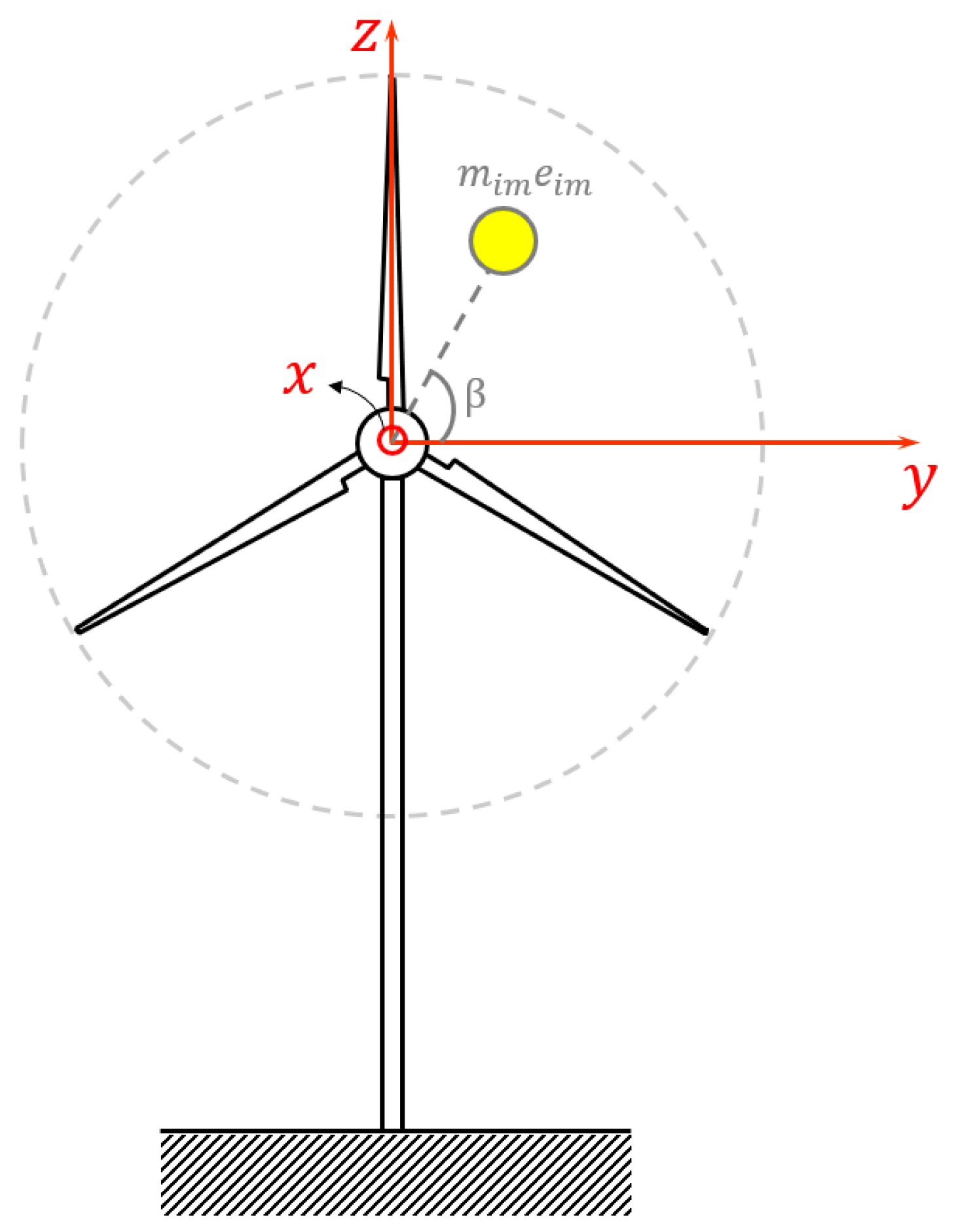
2.1. Nonstationary Equations of Motion

Figure 1 illustrates the schematic views for a shaft–disc system as a representative of an arbitrary unbalanced rotor.

The fixed coordinate system $x-y-z$ is attached to the shaft left support. The non-inertial coordinate system $\xi -\eta -\zeta$ is also attached to the shaft centerline. Considering that the torsional load and the rotational speed are time-varying parameters, the stationary coupled flexural–torsional unbalance model, introduced by Askari et al. [36], is updated for the nonstationary conditions as follows:

$$\delta u:EA{u}^{″}+C_u\dot{u}+\left[\rho A+\left(M_d+m_{im}\right)H\left(x-x_d\right)\right]\ddot{u}=0,$$

(1)

$$\begin{array}{c}\delta v:E{I}_{sh}{v}^{″″}+C_v\dot{v}+\left[\rho A+\left(M_d+m_{im}\right)H\left(x-x_d\right)\right]\ddot{v}\\ -\left[\rho I_{sh}+I_{d}H\left(x-x_d\right)\right]({\ddot{v}}^{″}+2\mathsf{\Omega }{\dot{w}}^{″}+2\ddot{\phi }{w}^{″}+2\dot{\mathsf{\Omega }}{w}^{″}\\ +2{\ddot{\phi }}^{\prime }{w}^{\prime }+2{\dot{\phi }}^{\prime }{\dot{w}}^{\prime }+2\dot{\phi }{\dot{w}}^{″})\\ =m_{im}{e}_{im}H(x\\ -x_d\left)\right[\left({\mathsf{\Omega }}^2+2\mathsf{\Omega }\dot{\phi }\right)\mathrm{c}\mathrm{o}\mathrm{s}\left({\int }_0^t\mathsf{\Omega }\mathrm{d}t\right)\\ +\left(\ddot{\phi }+\dot{\mathsf{\Omega }}-{\mathsf{\Omega }}^2\phi \right)\mathrm{s}\mathrm{i}\mathrm{n}\left({\int }_0^t\mathsf{\Omega }\mathrm{d}t\right)],\end{array}$$

(2)

$$\begin{array}{c}\delta w:E{I}_{sh}{w}^{″″}+C_w\dot{w}+\left[\rho A+\left(M_d+m_{im}\right)H\left(x-x_d\right)\right]\ddot{w}\\ -\left[\rho I_{sh}+I_{d}H\left(x-x_d\right)\right]\left({\ddot{w}}^{″}-2\mathsf{\Omega }{\dot{v}}^{″}-2{\dot{\phi }}^{\prime }{\dot{v}}^{\prime }-2\dot{\phi }{\dot{v}}^{″}\right)\\ =m_{im}{e}_{im}H\left(x-x_d\right)[\left({\mathsf{\Omega }}^2+2\mathsf{\Omega }\dot{\phi }\right)\mathrm{s}\mathrm{i}\mathrm{n}\left({\int }_0^t\mathsf{\Omega }\mathrm{d}t\right)\\ -\left(\ddot{\phi }+\dot{\mathsf{\Omega }}-{\mathsf{\Omega }}^2\phi \right)\mathrm{c}\mathrm{o}\mathrm{s}\left({\int }_0^t\mathsf{\Omega }\mathrm{d}t\right)],\end{array}$$

(3)

$$\begin{array}{c}\delta \phi :-G{J}_{sh}{\phi }^{″}+C_{\phi }\dot{\phi }+m_{im}{e}_{im}^{2}H\left(x-x_d\right)\left(\ddot{\phi }+\dot{\mathsf{\Omega }}\right)+\left[\rho J_{sh}+J_{d}H\left(x-x_d\right)\right]\left(\ddot{\phi }+\dot{\mathsf{\Omega }}+{\ddot{v}}^{\prime }{w}^{\prime }+\dot{v}\prime \dot{w}\prime \right)=T_{L}H(x-\\ x_T)+m_{im}{e}_{im}H\left(x-x_d\right)\left[\ddot{v}\mathrm{s}\mathrm{i}\mathrm{n}\left({\int }_0^t\mathsf{\Omega }\mathrm{d}t\right)-\ddot{w}\mathrm{c}\mathrm{o}\mathrm{s}\left({\int }_0^t\mathsf{\Omega }\mathrm{d}t\right)\right].\end{array}$$

(4)

where t is the time; the prime and dot signs denote partial differentiation with respect to x and t, respectively; the dependent variables u, v, w, and $\phi$ refer to the axial, lateral, transversal, and torsional displacements of the system, respectively; $\Omega$ denotes the time-varying rotational speed; and $T_L$ is the variable torsional load. The angle $\beta$ in Figure 1 refers to the torsional displacement, superimposed over the rigid-body rotation [36]. $\rho$, E, G, A, $I_{sh}$, and $J_{sh}$ are the density, modulus of elasticity, shear modulus, cross-sectional area, second moment of the cross-sectional area, and polar second moment of the cross-sectional area of the shaft, respectively; $C_u$, $C_v$, $C_w$, and $C_{\phi }$ are the axial, lateral, transversal, and torsional damping coefficients; $M_d$, $I_d$, and $J_d$ are the mass, the mass moment of inertia, and the polar mass moment of inertia of the disc, respectively; $x_d$ and $x_T$ denote the locations of the disc and the torsional load, respectively; $m_{im}$ is the unbalance mass placed at the distance $e_{im}$ from the rotation center; and $H\left(x\right)$ is the Heaviside function.

In view of the fact that any continuous function can be approximated by piecewise linear functions [41,42], the entire time-domain signal is segmented into intervals where the torsional load is linearly approximated over time:

$$T_L\left(t\right)=T_0+T_{1}t\mathrm{F}\mathrm{o}\mathrm{r}{t}_i\le t<t_{i+1},$$

(5)

where $T_0$ and $T_1$ are the constant torque and the torque rate of change in N.m and N.m/s over the interval [$t_i,t_{i+1}$], (i = 1, 2, 3, …), respectively.

Given Newton’s second law for rigid body rotational motion [11], i.e., $M=J\alpha$, where $M$ is the net torsional load acting on the system in N.m, $J$ is the equivalent rotary inertia of the system in kg.m², and $\alpha$ is the rotational acceleration in Rad/s², linear variation in the torsional load implies second-order nonlinear variation for the rotational speed. That is, the rotational speed over the interval [$t_i,t_{i+1}$] (i = 1, 2, 3, …) takes the form of

$$\mathsf{\Omega }\left(t\right)=2\pi \left(f_0+f_{1}t+f_2{t}^2\right)\mathrm{F}\mathrm{o}\mathrm{r}{t}_i\le t<t_{i+1},$$

(6)

where $f_0$ is the initial constant rotational speed in Hz over the time interval [$t_i,t_{i+1}$], (i = 1, 2, 3, …). $f_1$ also denotes the chirp rate in Hz/s over that interval and $f_2$ is the variation of the chirp rate in Hz/s over that interval.

As seen from Equations (1)–(4), the axial motion is independent from the torsional and flexural dynamics of the system. Focusing on the coupled flexural–torsional dynamics of the system, assuming the first mode only contributes to system dynamics [36], and following the Galerkin weighted residual method [37,38] for simply supported boundary conditions with sinusoidal basis functions [36], the reduced flexural–torsional governing equations of motion over the ith time segment take the form of

$$\begin{array}{c}{K}_y{v}_{mid}+C_y{\dot{v}}_{mid}+M_y{\ddot{v}}_{mid}+{2\pi B}_1\left[\left(f_0+f_{1}t+f_2{t}^2\right){\dot{w}}_{mid}+\left(f_1+{2f}_{2}t\right)w_{mid}\right]\\ +B_2\left({\ddot{\phi }}_{mid}{w}_{mid}+{\dot{\phi }}_{mid}{\dot{w}}_{mid}\right)\\ =m_{im}{e}_{im}\left\{\right[{4{\pi }^2\left(f_0+f_{1}t+f_2{t}^2\right)}^2\\ +4\pi \left(f_0+f_{1}t+f_2{t}^2\right)\mathrm{s}\mathrm{i}\mathrm{n}\left({\displaystyle \frac{\pi x_d}{L}}\right){\dot{\phi }}_{mid}\left]\mathrm{c}\mathrm{o}\mathrm{s}\right[2\pi (f_{0}t+{\displaystyle \frac{1}{2}}{f}_1{t}^2\\ +{\displaystyle \frac{1}{3}}{f}_2{t}^3)+{\theta }_0]\\ +[\left[{\ddot{\phi }}_{mid}-{4{\pi }^2\left(f_0+f_{1}t+f_2{t}^2\right)}^2{\phi }_{mid}\right]sin\left({\displaystyle \frac{\pi x_d}{L}}\right)\\ +2\pi \left(f_1+{2f}_{2}t\right)]\mathrm{s}\mathrm{i}\mathrm{n}2\pi \left(f_{0}t+{\displaystyle \frac{1}{2}}{f}_1{t}^2+{\displaystyle \frac{1}{3}}{f}_2{t}^3\right)\\ +{\theta }_0\left]\right\}\mathrm{s}\mathrm{i}\mathrm{n}\left({\displaystyle \frac{\pi x_d}{L}}\right),\end{array}$$

(7)

$$\begin{array}{c}{K}_z{w}_{mid}+C_z{\dot{w}}_{mid}+M_z{\ddot{w}}_{mid}-{2\pi B}_1\left(f_0+f_{1}t+f_2{t}^2\right){\dot{v}}_{mid}-B_2{\dot{\phi }}_{mid}{\dot{v}}_{mid}\\ =m_{im}{e}_{im}\left\{\right[4{\pi }^2{\left(f_0+f_{1}t+f_2{t}^2\right)}^2\\ +4\pi \left(f_0+f_{1}t+f_2{t}^2\right)sin\left({\displaystyle \frac{\pi x_d}{L}}\right){\dot{\phi }}_{mid}\left]sin\right[2\pi (f_{0}t+{\displaystyle \frac{1}{2}}{f}_1{t}^2\\ +{\displaystyle \frac{1}{3}}{f}_2{t}^3)+{\theta }_0]\\ -[\left[{\ddot{\phi }}_{mid}-{4{\pi }^2\left(f_0+f_{1}t+f_2{t}^2\right)}^2{\phi }_{mid}\right]sin\left({\displaystyle \frac{\pi x_d}{L}}\right)\\ +2\pi \left(f_1+{2f}_{2}t\right)\left]cos\right[2\pi \left(f_{0}t+{\displaystyle \frac{1}{2}}{f}_1{t}^2+{\displaystyle \frac{1}{3}}{f}_2{t}^3\right)\\ +{\theta }_0\left]\right\}\mathrm{s}\mathrm{i}\mathrm{n}\left({\displaystyle \frac{\pi x_d}{L}}\right),\end{array}$$

(8)

$$\begin{array}{c}{K}_t{\phi }_{mid}+C_t{\dot{\phi }}_{mid}+M_t{\ddot{\phi }}_{mid}+B_3\left({\ddot{v}}_{mid}{w}_{mid}+{\dot{v}}_{mid}{\dot{w}}_{mid}\right)+B_4\left(f_1+{2f}_{2}t\right)\\ =\left(T_{1}t+T_0\right)\mathrm{s}\mathrm{i}\mathrm{n}\left({\displaystyle \frac{\pi x_T}{L}}\right)\\ +m_{im}{e}_{im}\{{\ddot{v}}_{mid}sin\left[2\pi \left(f_{0}t+{\displaystyle \frac{1}{2}}{f}_1{t}^2+{\displaystyle \frac{1}{3}}{f}_2{t}^3\right)+{\theta }_0\right]\\ -{\ddot{w}}_{mid}cos\left[2\pi \left(f_{0}t+{\displaystyle \frac{1}{2}}{f}_1{t}^2+{\displaystyle \frac{1}{3}}{f}_2{t}^3\right)+{\theta }_0\right]\}{\mathrm{s}\mathrm{i}\mathrm{n}}^2\left({\displaystyle \frac{\pi x_d}{L}}\right).\end{array}$$

(9)

where ${\theta }_0$ is the initial angle of unbalance in Rad over the ith time interval (i = 1, 2, 3, …).

The model coefficients are also given by

$$\begin{gathered} K_y=E{I}_{sh}{\left({\displaystyle \frac{\pi }{L}}\right)}^4{\int }_0^L{sin}^2\left({\displaystyle \frac{\pi x}{L}}\right)dx,{C_y=C}_v{\int }_0^L{sin}^2\left({\displaystyle \frac{\pi x}{L}}\right)dx, \\ \begin{array}{cc}{M}_y& =\rho A{\int }_0^L{sin}^2\left({\displaystyle \frac{\pi x}{L}}\right)dx+\left(M_d+m_{im}\right){\mathrm{s}\mathrm{i}\mathrm{n}}^2\left({\displaystyle \frac{\pi x_d}{L}}\right)\hfill \\ & +\rho I_{sh}{\left({\displaystyle \frac{\pi }{L}}\right)}^2{\int }_0^L{sin}^2\left({\displaystyle \frac{\pi x}{L}}\right)dx+{{\left({\displaystyle \frac{\pi }{L}}\right)}^2{sin}^2\left({\displaystyle \frac{\pi x_d}{L}}\right)I}_d,\hfill \end{array} \\ {B}_1=2{\left({\displaystyle \frac{\pi }{L}}\right)}^2\left[\rho I_{sh}{\int }_0^L{sin}^2\left({\displaystyle \frac{\pi x}{L}}\right)dx+I_d{\mathrm{s}\mathrm{i}\mathrm{n}}^2\left({\displaystyle \frac{\pi x_d}{L}}\right)\right], \\ \begin{array}{cc}{B}_2=& -2\rho I_{sh}{\left({\displaystyle \frac{\pi }{L}}\right)}^2{\int }_0^L\left[{cos}^2\left({\displaystyle \frac{\pi x}{L}}\right)sin\left({\displaystyle \frac{\pi x}{L}}\right)-{sin}^3\left({\displaystyle \frac{\pi x}{L}}\right)\right]dx\hfill \\ & -2{{\left({\displaystyle \frac{\pi }{L}}\right)}^2\left[{cos}^2\left({\displaystyle \frac{\pi x_d}{L}}\right)sin\left({\displaystyle \frac{\pi x_d}{L}}\right)-{sin}^3\left({\displaystyle \frac{\pi x_d}{L}}\right)\right]I}_d,\hfill \end{array} \\ {K}_z=E{I}_{sh}{\left({\displaystyle \frac{\pi }{L}}\right)}^4{\int }_0^L{sin}^2\left({\displaystyle \frac{\pi x}{L}}\right)dx,{C_z=C}_w{\int }_0^L{sin}^2\left({\displaystyle \frac{\pi x}{L}}\right)dx, \\ \begin{array}{cc}{M}_z& =\rho A{\int }_0^L{sin}^2\left({\displaystyle \frac{\pi x}{L}}\right)dx+\left(M_d+m_{im}\right){\mathrm{s}\mathrm{i}\mathrm{n}}^2\left({\displaystyle \frac{\pi x_d}{L}}\right)\hfill \\ & +\rho I_{sh}{\left({\displaystyle \frac{\pi }{L}}\right)}^2{\int }_0^L{sin}^2\left({\displaystyle \frac{\pi x}{L}}\right)dx+{{\left({\displaystyle \frac{\pi }{L}}\right)}^2{sin}^2\left({\displaystyle \frac{\pi x_d}{L}}\right)I}_d,\hfill \end{array} \\ {K}_t={G{J}_{sh}\left({\displaystyle \frac{\pi }{L}}\right)}^2{\int }_0^L{sin}^2\left({\displaystyle \frac{\pi x}{L}}\right)dx,C_t=C_{\phi }{\int }_0^L{sin}^2\left({\displaystyle \frac{\pi x}{L}}\right)dx, \\ {M}_t=\rho J_{sh}{\int }_0^L{sin}^2\left({\displaystyle \frac{\pi x}{L}}\right)dx+J_d{\mathrm{s}\mathrm{i}\mathrm{n}}^2\left({\displaystyle \frac{\pi x_d}{L}}\right)+m_{im}{e}_{im}^2{\mathrm{s}\mathrm{i}\mathrm{n}}^2\left({\displaystyle \frac{\pi x_d}{L}}\right), \\ {B}_3=\rho {J_{sh}\left({\displaystyle \frac{\pi }{L}}\right)}^2{\int }_0^L{cos}^2\left({\displaystyle \frac{\pi x}{L}}\right)sin\left({\displaystyle \frac{\pi x}{L}}\right)dx+{J_{d}cos}^2\left({\displaystyle \frac{\pi x_d}{L}}\right)sin\left({\displaystyle \frac{\pi x_d}{L}}\right), \\ {B}_4=2\pi \left[\rho J_{sh}{\int }_0^{L}sin\left({\displaystyle \frac{\pi x}{L}}\right)dx+J_{d}sin\left({\displaystyle \frac{\pi x_d}{L}}\right)+m_{im}{e}_{im}^{2}sin\left({\displaystyle \frac{\pi x_d}{L}}\right)\right]. \end{gathered}$$

(10)

2.2. Solution Procedure

Equations (7)–(9) govern the nonstationary coupled flexural–torsional dynamics of an unbalanced rotor. This system of equations is solved numerically using the fourth-order Runge–Kutta method [42,43,44,45]. To this end, this system of three second-order initial value problems is rewritten in matrix form so that the second-order derivatives remain on the left-hand side, and all the other terms are moved to the right-hand side of the equations. Doing so, one gets

$$\left[\begin{array}{ccc}{\mathit{A}}_{11}& {\mathit{A}}_{12}& {\mathit{A}}_{13}\\ {\mathit{A}}_{21}& {\mathit{A}}_{22}& {\mathit{A}}_{23}\\ {\mathit{A}}_{31}& {\mathit{A}}_{32}& {\mathit{A}}_{33}\end{array}\right]\left\{\begin{array}{c}{\ddot{v}}_{mid}\\ {\ddot{w}}_{mid}\\ {\ddot{\phi }}_{mid}\end{array}\right\}=\left\{\begin{array}{c}{\mathit{b}}_1\\ {\mathit{b}}_2\\ {\mathit{b}}_3\end{array}\right\},$$

(11)

where

$$\begin{gathered} {\mathit{A}}_{11}=M_y,{\mathit{A}}_{12}=0, \\ {\mathit{A}}_{13}=B_2{w}_{mid}-m_{im}{e}_{im}{\mathrm{s}\mathrm{i}\mathrm{n}}^2\left({\displaystyle \frac{\pi x_d}{L}}\right)\mathrm{s}\mathrm{i}\mathrm{n}\left[2\pi \left(f_{0}t+{\displaystyle \frac{1}{2}}{f}_1{t}^2+{\displaystyle \frac{1}{3}}{f}_2{t}^3\right)+{\theta }_0\right], \\ {\mathit{A}}_{21}=0,{\mathit{A}}_{22}=M_z, \\ {\mathit{A}}_{23}=m_{im}{e}_{im}{\mathrm{s}\mathrm{i}\mathrm{n}}^2\left({\displaystyle \frac{\pi x_d}{L}}\right)\mathrm{c}\mathrm{o}\mathrm{s}\left[2\pi \left(f_{0}t+{\displaystyle \frac{1}{2}}{f}_1{t}^2+{\displaystyle \frac{1}{3}}{f}_2{t}^3\right)+{\theta }_0\right], \\ {\mathit{A}}_{31}=B_3{w}_{mid}-m_{im}{e}_{im}\mathrm{s}\mathrm{i}\mathrm{n}\left[2\pi \left(f_{0}t+{\displaystyle \frac{1}{2}}{f}_1{t}^2+{\displaystyle \frac{1}{3}}{f}_2{t}^3\right)+{\theta }_0\right]{\mathrm{s}\mathrm{i}\mathrm{n}}^2\left({\displaystyle \frac{\pi x_d}{L}}\right), \\ {\mathit{A}}_{32}=m_{im}{e}_{im}\mathrm{c}\mathrm{o}\mathrm{s}\left[2\pi \left(f_{0}t+{\displaystyle \frac{1}{2}}{f}_1{t}^2+{\displaystyle \frac{1}{3}}{f}_2{t}^3\right)+{\theta }_0\right]{\mathrm{s}\mathrm{i}\mathrm{n}}^2\left({\displaystyle \frac{\pi x_d}{L}}\right),{\mathit{A}}_{33}=M_t, \\ \begin{array}{c}{\mathit{b}}_1=-K_y{v}_{mid}-C_y{\dot{v}}_{mid}-{2\pi B}_1\left[\left(f_0+f_{1}t+f_2{t}^2\right){\dot{w}}_{mid}+\left(f_1+2f_{2}t\right)w_{mid}\right]\\ -B_2\left({\ddot{\phi }}_{mid}{w}_{mid}+{\dot{\phi }}_{mid}{\dot{w}}_{mid}\right)\\ +m_{im}{e}_{im}\left\{\right[{4{\pi }^2\left(f_0+f_{1}t+f_2{t}^2\right)}^2\\ +4\pi \left(f_0+f_{1}t+f_2{t}^2\right)\mathrm{s}\mathrm{i}\mathrm{n}\left({\displaystyle \frac{\pi x_d}{L}}\right){\dot{\phi }}_{mid}\left]\mathrm{c}\mathrm{o}\mathrm{s}\right[2\pi (f_{0}t+{\displaystyle \frac{1}{2}}{f}_1{t}^2\\ +{\displaystyle \frac{1}{3}}{f}_2{t}^3)+{\theta }_0]\\ +[-{4{\pi }^2\left(f_0+f_{1}t+f_2{t}^2\right)}^{2}sin\left({\displaystyle \frac{\pi x_d}{L}}\right){\phi }_{mid}\\ +2\pi \left(f_1+{2f}_{2}t\right)\left]\mathrm{s}\mathrm{i}\mathrm{n}\right[2\pi \left(f_{0}t+{\displaystyle \frac{1}{2}}{f}_1{t}^2+{\displaystyle \frac{1}{3}}{f}_2{t}^3\right)\\ +{\theta }_0\left]\right\}\mathrm{s}\mathrm{i}\mathrm{n}\left({\displaystyle \frac{\pi x_d}{L}}\right),\end{array} \\ \begin{array}{c}{\mathit{b}}_2={-K}_z{w}_{mid}-C_z{\dot{w}}_{mid}+{2\pi B}_1\left(f_0+f_{1}t+f_2{t}^2\right){\dot{v}}_{mid}+B_2{\dot{\phi }}_{mid}{\dot{v}}_{mid}\\ +m_{im}{e}_{im}\left\{\right[4{\pi }^2{\left(f_0+f_{1}t+f_2{t}^2\right)}^2\\ +4\pi \left(f_0+f_{1}t+f_2{t}^2\right)sin\left({\displaystyle \frac{\pi x_d}{L}}\right){\dot{\phi }}_{mid}\left]sin\right[2\pi (f_{0}t+{\displaystyle \frac{1}{2}}{f}_1{t}^2\\ +{\displaystyle \frac{1}{3}}{f}_2{t}^3)+{\theta }_0]\\ -[{-4{\pi }^2\left(f_0+f_{1}t+f_2{t}^2\right)}^{2}sin\left({\displaystyle \frac{\pi x_d}{L}}\right){\phi }_{mid}\\ +2\pi \left(f_1+{2f}_{2}t\right)\left]cos\right[2\pi \left(f_{0}t+{\displaystyle \frac{1}{2}}{f}_1{t}^2+{\displaystyle \frac{1}{3}}{f}_2{t}^3\right)\\ +{\theta }_0\left]\right\}\mathrm{s}\mathrm{i}\mathrm{n}\left({\displaystyle \frac{\pi x_d}{L}}\right),\end{array} \\ {\mathit{b}}_3=-K_t{\phi }_{mid}-C_t{\dot{\phi }}_{mid}-B_3{\dot{v}}_{mid}{\dot{w}}_{mid}-B_4\left(f_1+{2f}_{2}t\right)+\left(T_{1}t+T_0\right)\mathrm{s}\mathrm{i}\mathrm{n}\left({\displaystyle \frac{\pi x_T}{L}}\right). \end{gathered}$$

(12)

Multiplying both sides of Equation (11) by ${\mathbf{A}}^{-1}$ and rewriting the resulting equations in the form of a system of six first-order differential equations [36], the solutions were obtained via MATLAB, version R2024a, command ODE45. Given the fact that the vibration sensors provide accelerations, the acceleration signals are finally determined by adopting Equation (11) together with the zeroth and the first derivatives of the independent variables, which are already available as the output of the MATLAB command ODE45.

In view of the fact that the unbalance fault signature is reflected on the axes, which are perpendicular to the shaft direction, the acceleration signal should be considered along either the y or the z axes [33]. There is no difference between these two directions from a theoretical point of view because the shaft cross-section is symmetric. However, in practice, the signature of the unbalance fault can only be observed in the direction whose corresponding support stiffness is lower [33]. Therefore, just for the sake of brevity, the acceleration signal along the y-axis, which is along the horizon, is only considered in this study [36].

Considering the nonstationary acceleration signal in y direction, the magnitude of the fundamental rotational harmonic is obtained by adopting the higher-order STCFT [39], which is effectively utilized for fault diagnosis in nonstationary conditions [46,47]. This transform states

$$V\left(f,\tilde{T}\right)={\displaystyle \frac{1}{T}}{\int }_{-\infty }^{+\infty }h\left(t-\tilde{T}\right){\ddot{v}}_{mid}\left(t\right)e^{-2\pi j\left({\int }_0^{t}f\left(\tau \right)d\tau \right)}dt,$$

(13)

where $j=\sqrt{-1}$, and $h\left(t\right)$ is the time window with the duration of T and the center of $\tilde{T}$; here, the Hamming time window is chosen. $f\left(\tau \right)$ is the instantaneous rotational speed in Hz: $f\left(\tau \right)=f_0+f_1\tau +f_2{\tau }^2$.

Taking the higher-order STCFT from the transversal acceleration signal, the magnitude of the frequency component, which is the closest one to the rotational speed, is extracted as the conventional unbalance fault indicator S. Next, the speed-invariant unbalance diagnostic feature $S_N$ is obtained by [33]

$$S_N={\displaystyle \frac{S}{{\overline{f}}^4}}.$$

(14)

where $\overline{f}$ is the mean rotational speed over each time window. The unit of S is m/s², and so the unit of S_N becomes m.s².

3. Experimental Analysis

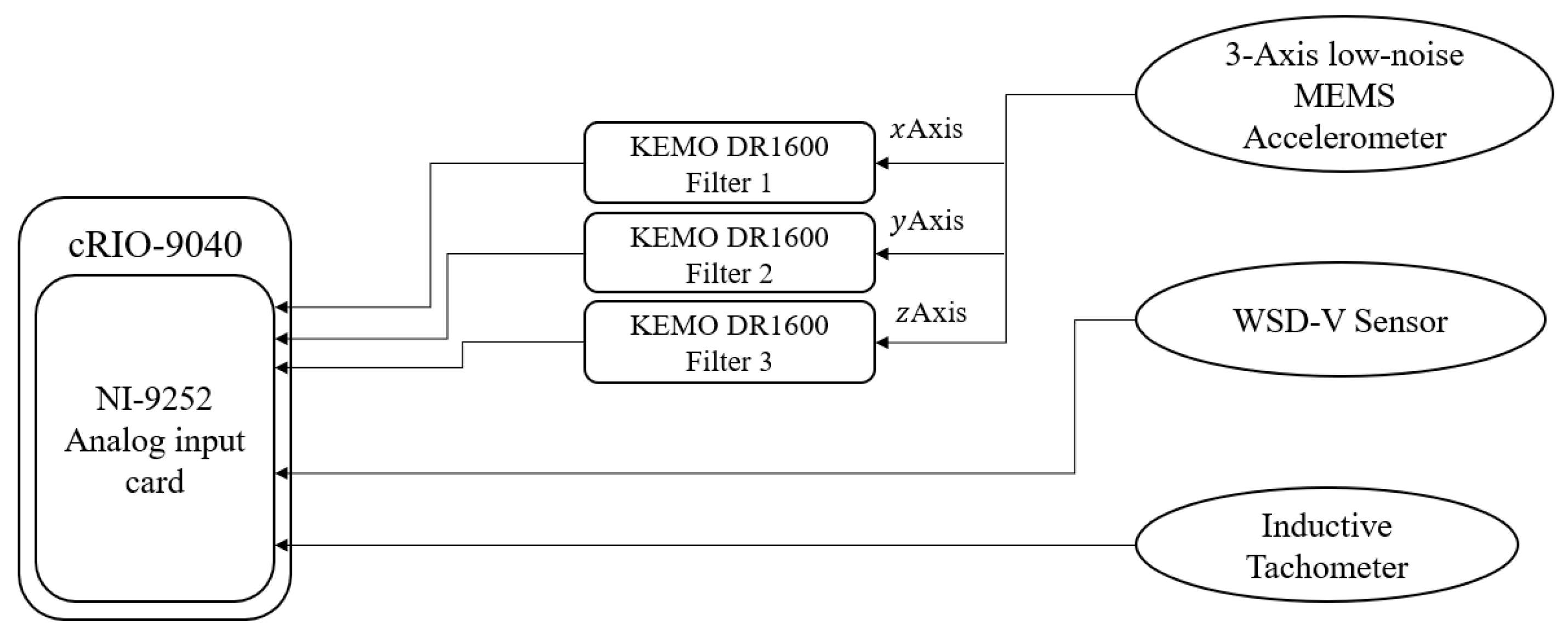
3.1. Experimental Setup

A variable-speed 2.3 MW wind turbine, operating within a permissible unbalance threshold of 5.94 × 10⁸ gr·mm [1,2,33], was used to validate the theory. This turbine is a horizontal-axis machine with three blades of 40 m length. The vibration, rotational speed, and wind speed data were collected over a long period of time to cover a broad range of wind and rotational speeds.

The data were collected using a system comprising a three-axial MEMS accelerometer, three KEMO filters, an inductive tachometer, a wind speed and direction sensor, and a data acquisition unit. The data acquisition unit, depicted schematically in Figure 2, was mounted within the turbine’s nacelle housing.

Two MEMS accelerometers, (a) ADXL354B and (b) PCB 3743F112G, whose details have been given in Table 2 of Ref. [33], were hired. The accelerometers were installed on the wind turbine’s main bearing so that they are as close as possible to the blades, the most vulnerable parts to the unbalance fault. The accelerometers were fed by 5 V voltage supplied from the USB A port on the cRIO—9040 system, whose details are given below. Figure 3 illustrates the directions of the accelerometer axes. As this figure depicts, the accelerometer coordinate system is set so that their x-axes are along the wind turbine’s main shaft, pointing outward. The y-axes are perpendicular to the wind turbine’s main shaft along the horizontal axis pointing to the right. The z-axes are towards the vertical direction, pointing upward.

The accelerometers’ outputs were amplified, and their frequency bandwidths were delimitated by using DR 1600 KEMO anti-aliasing filters. These filters have a power consumption of 3 W and operate at a supply voltage of 24 V. They function effectively within a temperature range of −10 °C to 45 °C, feature a bandwidth of 500 kHz, and exhibit total harmonic distortion below 0.003%. The filters are tunable to cover a broad gain range of $\times 1$, $\times 2$, $\times 5$, …, $\times 1000$. The gain and the cut-off frequencies of these adjustable filters were set to $\times 10$ and 10 kHz, respectively.

An LJ12A3-4-Z/BY inductive proximity sensor with 32 pulses per revolution was employed to measure the wind turbine’s main shaft’s rotational speed. This sensor features a detection distance of up to 4 mm, responds at frequencies up to 500 Hz, and functions reliably between −25 °C and 55 °C.

The wind speed data was measured via an MSL WSD-V sensor, which was fed by 24 V voltage. The sensor’s head unit functions reliably between −20 °C and 60 °C and is capable of measuring wind speeds between 0.5 m/s and 50 m/s, offering an accuracy of ±1.5 m/s and a resolution finer than 0.5 m/s. Notably, the output voltage ranges from 0 to 10 V, which was scaled so that 0 V is equivalent to 0 m/s and 10 V is equivalent to 50 m/s. In addition, the threshold for starting to operate was 0.5 m/s.

The analog outputs of the sensors are simultaneously sampled with a rate of 25 kS/s via an NI-9252 web DAQ card installed on a cRIO-9040 system, whose maximum input/output frequency is 20 MHz. This web DAQ card has eight inputs and provides 24-bit resolution with the maximum sampling rate of 50 kS/s. It can operate within the temperature range from −20 °C to 52 °C.

3.2. Processing Experimental Signals

As mentioned earlier, the higher-order STCFT, which is given in Equation (13), is adopted in this study to process the nonstationary wind turbine signals. Apart from the vibration signal, this technique requires the shaft rotational speed signal as well. The shaft rotational speed is extracted from the tachometer signal via the elapsed time method [48]. Processing the vibration signal in y direction, the net peak value, associated with the fundamental rotational harmonic, needs to be obtained. To this end, the mean noise level is calculated by averaging the intensities of the frequency components around the fundamental rotational harmonic peak that are contributing to the surrounding noise, not other stable peaks in the neighborhood of the fundamental peak. Therefore, the average surrounding noise level is given by [33,36,49]

$$N_{ave}={\displaystyle \frac{\sum _{i=1}^n{N}_i^{left}+\sum _{i=1}^n{N}_i^{right}}{2n}},$$

(15)

where $N_i^{\mathrm{l}\mathrm{e}\mathrm{f}\mathrm{t}}$ and $N_i^{\mathrm{r}\mathrm{i}\mathrm{g}\mathrm{h}\mathrm{t}}$ denote the magnitude of the ith component from the peak on its left- and right-hand sides, respectively.

It is found that the immediate component before and after the fundamental peak is influenced by that peak. So, excluding the immediate neighbors of the fundamental rotational harmonic peak, three frequency components on either side are selected and averaged, resulting in a total of six frequency components. Doing so, the net peak value becomes [33,36,49]

$$P_{net}=\sqrt{P^2-N_{ave}^2},$$

(16)

where P is the peak value.

For obtaining a signal-to-noise ratio related to the fundamental harmonic, the net peak value is normalized by the local interference level (i.e., $N_{ave}$); thus, the normalized conventional unbalance fault indicator (i.e., $\overline{S}$) is as follows:

$$\overline{S}={\displaystyle \frac{P_{net}}{N_{ave}}}.$$

(17)

The normalized version of the proposed speed-invariant unbalance diagnostic feature (${\overline{S}}_N$) is also given by [33]

$${\overline{S}}_N={\displaystyle \frac{\overline{S}}{{\overline{f}}^4}}.$$

(18)

Since $\overline{S}$ is dimensionless, the unit of ${\overline{S}}_N$ becomes Hz⁻⁴ or s⁴ [33,36].

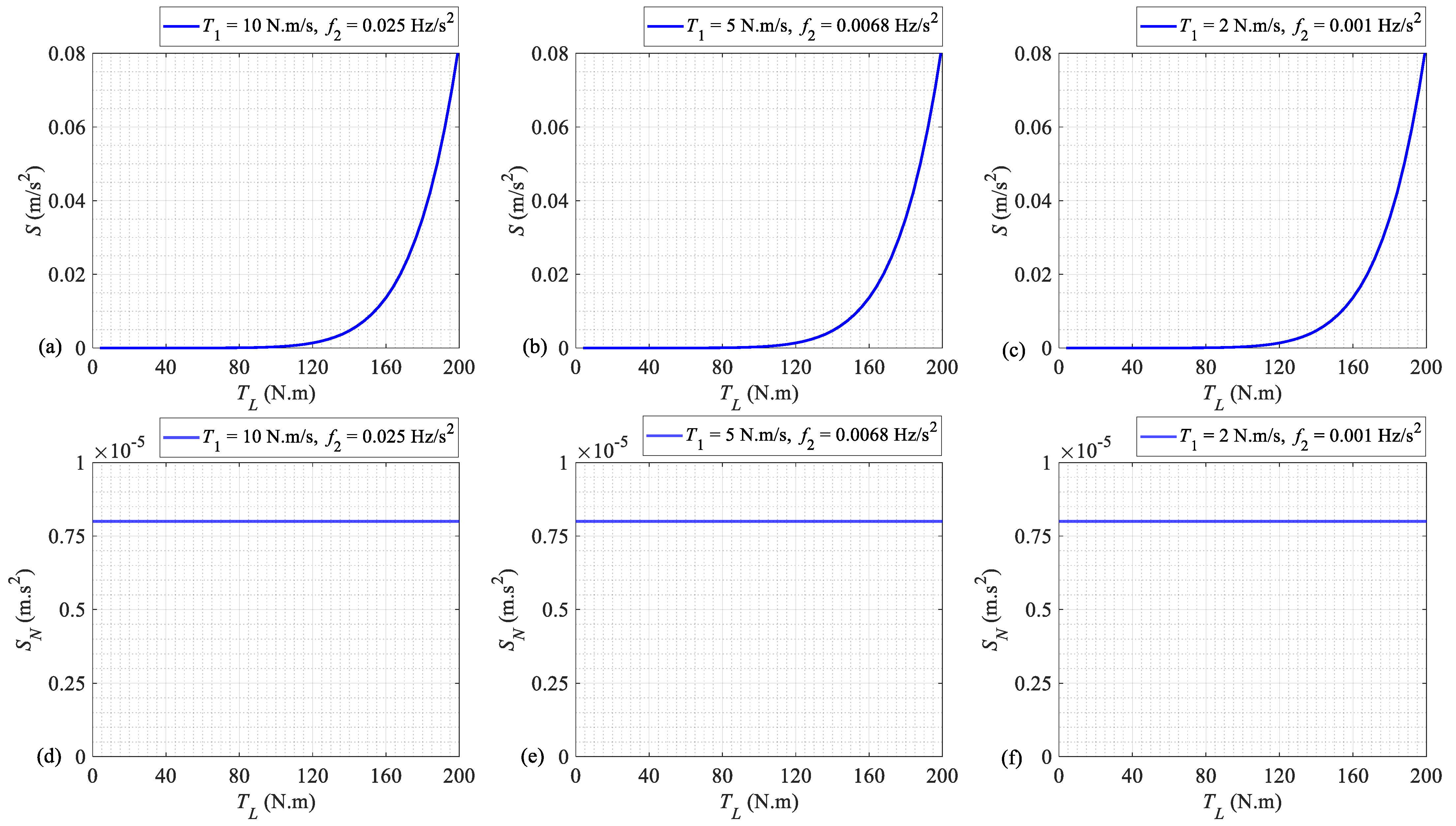
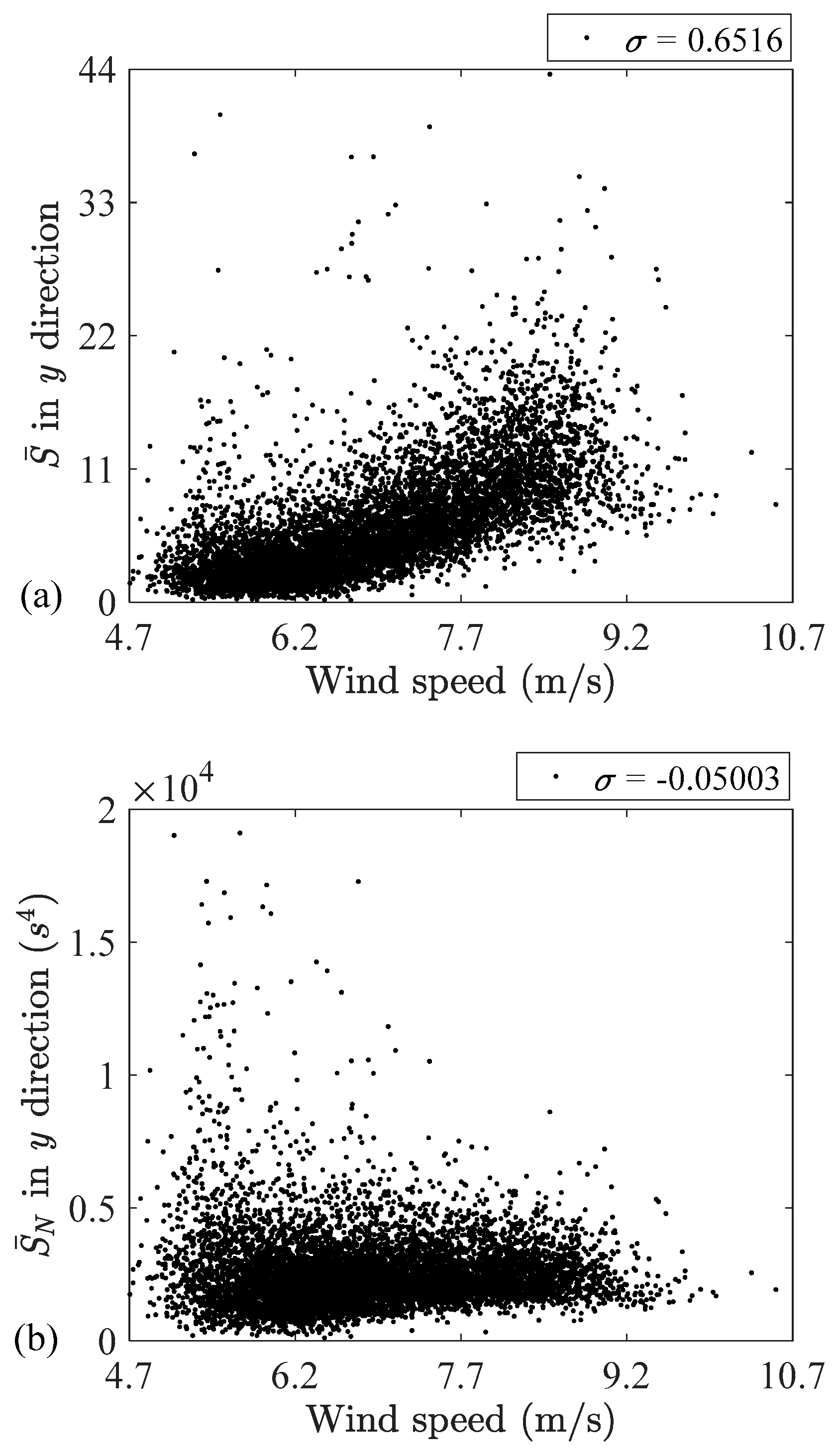
4. Results and Discussion

Given the universality of the present theoretical model, numerical results were obtained for a typical steel disc–shaft system with the specifications provided in

Table 1. Specifications of the disc–shaft system.

$\mathit{L}\left(\mathbf{m}\right)$	$\mathit{r}\left(\mathbf{m}\right)$	${\mathit{r}}_{\mathit{d}}\left(\mathbf{m}\right)$	$\mathit{\rho }\left(\mathbf{k}\mathbf{g}/{\mathbf{m}}^3\right)$	$\mathit{E}\left(\mathbf{G}\mathbf{P}\mathbf{a}\right)$	$\mathit{G}\left(\mathbf{G}\mathbf{P}\mathbf{a}\right)$	${\mathit{M}}_{\mathit{d}}\left(\mathbf{k}\mathbf{g}\right)$	${\mathit{m}}_{\mathit{i}\mathit{m}}\left(\mathbf{k}\mathbf{g}\right)$	${\mathit{e}}_{\mathit{i}\mathit{m}}\left(\mathbf{m}\right)$
1	0.03	0.15	7870	206	79	50	0.5	0.12

. It is assumed that the disc is located at the middle of the shaft, and the torque is also applied there.

Assuming that the present disc–shaft system is operating under 200 N.m nominal torque and 10 Hz nominal speed [36], the run-up process, in which the rotor starts from rest and the torsional load increases from zero to 200 N.m, is considered. To obtain the numerical results, three different load rates of $T_1=10,5,\mathrm{a}\mathrm{n}\mathrm{d}2\mathrm{N}.\mathrm{m}/\mathrm{s}$ are taken into account. Given starting from rest and the linear variation in the torque over the run-up process (see Equation (5)), the run-up times for the three cases mentioned above are obtained as 20 s, 40 s, and 100 s, respectively. In view of a nominal speed of 10 Hz, starting from rest, and the parabolic variation of the rotational speed (see Equation (6)), the only non-zero frequency coefficient $f_2$ takes the values of 0.025, 0.0068, and 0.001 Hz/s², respectively.

Table 2. Different run-up processes assessed.

	${\mathit{T}}_0\left(\mathbf{N}.\mathbf{m}\right)$	${\mathit{T}}_1\left(\mathbf{N}.\mathbf{m}/\mathbf{s}\right)$	${\mathit{f}}_0\left(\mathbf{H}\mathbf{z}\right)$	${\mathit{f}}_1\left(\mathbf{H}\mathbf{z}/\mathbf{s}\right)$	${\mathit{f}}_2\left(\mathbf{H}\mathbf{z}/{\mathbf{s}}^2\right)$	Duration (s)	Chirp Rate (${\mathit{f}}_1+2{\mathit{f}}_2\mathit{t}$) (Hz/s)
Case 1	0	10	0	0	0.025	20	[0, 1]
Case 2	0	5	0	0	0.0068	40	[0, 0.5]
Case 3	0	2	0	0	0.001	100	[0, 0.2]

summarizes this information for the three run-up processes assessed. This table also represents the chirp rate ranges associated with all three cases. As is seen, the chirp rates vary from zero up to the maximum values of 1, 0.5, and 0.2 Hz/s, respectively. Notably, these chirp rates cover the variable chirp rate observable in wind turbine data, where it does not exceed 0.01 Hz/s [33].

Given the maximum chirp rate of 1 Hz/s, the acceleration signal is processed by selecting a 0.8 s time window and 50% overlapping. Notably, the window duration is selected just to avoid the changes in the rotational speed during a time window higher than the frequency resolution [50].

Figure 4 illustrates the variation in the conventional and proposed diagnostic features [33] versus the instantaneous torsional load for the three different torque rates and chirp rates. It is assumed that the damping coefficients ${\overline{\xi }}_y,{\overline{\xi }}_z,\mathrm{and}{\overline{\xi }}_t$ are the same and set to $\overline{\mathsf{\xi }}$ = 0.05, where ${\overline{\xi }}_i={\displaystyle \frac{C_i}{2\sqrt{M_i{K}_i}}},\left(i\equiv y,z,t\right)$ [51]. As this figure demonstrates, the magnitude of the fundamental rotational harmonic depends on the level of the torsional load in non-stationary conditions. This dependency is because of the dependency between the fundamental rotational harmonic intensity and the rotational speed as well as the dependency between the torsional load and the rotational speed, which is unavoidable in non-stationary conditions. However, as Figure 4d–f demonstrates, the proposed diagnostic feature is independent from the torsional load because it is speed-invariant. So, aside from speed-invariancy, it can be claimed that this feature is also load-invariant.

Table 3. Influence of damping on the proposed unbalance diagnostic feature [33], i.e., $S_N$, ($\mathrm{m}.{\mathrm{s}}^2$).

	${\mathit{T}}_1=10\frac{\mathbf{N}.\mathbf{m}}{\mathbf{s}},{\mathit{f}}_2=0.025\frac{\mathbf{H}\mathbf{z}}{{\mathbf{s}}^2}$	${\mathit{T}}_1=5\frac{\mathbf{N}.\mathbf{m}}{\mathbf{s}},{\mathit{f}}_2=0.0068\frac{\mathbf{H}\mathbf{z}}{{\mathbf{s}}^2}$	${\mathit{T}}_1=2\frac{\mathbf{N}.\mathbf{m}}{\mathbf{s}},{\mathit{f}}_2=0.001\frac{\mathbf{H}\mathbf{z}}{{\mathbf{s}}^2}.$
$\xi =0$	$0.81\times {10}^{-5}$	$0.81\times {10}^{-5}$	$0.81\times {10}^{-5}$
$\xi =0.05$	$0.80\times {10}^{-5}$	$0.80\times {10}^{-5}$	$0.80\times {10}^{-5}$
$\xi =0.1$	$0.80\times {10}^{-5}$	$0.80\times {10}^{-5}$	$0.80\times {10}^{-5}$
$\xi =0.2$	$0.80\times {10}^{-5}$	$0.80\times {10}^{-5}$	$0.80\times {10}^{-5}$
$\xi =0.4$	$0.79\times {10}^{-5}$	$0.79\times {10}^{-5}$	$0.79\times {10}^{-5}$

provides the values of the proposed speed-invariant diagnostic feature [33] at different torque and chirp rates for different damping ratios. As is seen, damping has no considerable effect on this feature. The reason behind this observation is that the ratio of the rotational speed to the resonance frequency in the unbalance diagnostic region, where the proposed diagnostic feature is also valid, is less than 20%. As discussed in [33], the damping has no considerable effect in this region.

Given the independency of the novel diagnostic feature [33] from speed and torsional load, and also the fact that it is almost independent from the damping ratio, it can be said that this fault indicator is suitable for unbalance diagnosis in all operational conditions.

To verify the theoretical conclusion related to the load independency of the proposed diagnostic feature [33], a 2.3 MW variable-speed wind turbine operating within an allowable unbalance threshold is considered. To cover as many different operational conditions as possible, the vibration data were collected over a sufficiently long period of time and saved in 60 min time portions. Setting the duration of the time window to 50 s and accounting for 40% overlapping, the normalized conventional (i.e., $\overline{S}$) and speed-invariant (i.e., ${\overline{S}}_N$) diagnostic features in the y-axis, which is placed within the blade rotational plane and takes the lower stiffness, are extracted [33]. Each feature (i.e., $\overline{S}$ or ${\overline{S}}_N$) comprises 8181 data points. Throughout the analysis period, the rotational speed ranges from 0.17 to 0.27 Hz, while the wind speed fluctuates between 4.7 and 10.7 m/s. Due to the nature of the system, where the wind speed continuously goes up and down, the wind turbine rotational speed chirp rate is variable, not exceeding 0.01 Hz/s.

Given the objective of validating the load independency of the diagnostic feature proposed in [33] and the universality of the theoretical framework presented, the extensive experimental campaign conducted on a 2.3 MW machine, representative of standard wind turbines found in wind farms, operating across a wide spectrum of wind conditions and rotational speeds, is deemed adequate for the experimental validation. Therefore, additional validation on other wind turbines is deemed unnecessary.

In addition to wind turbines, the dependency of the proposed unbalance diagnosis feature on torsional load has also been investigated for induction motors in a previous work [36]. As indicated in that study, the application of multiple loads causes the induction motor to operate under multiple rotational speeds. It was demonstrated there that employing the proposed speed-invariant unbalance technology ensures load independence in systems operating under multiple speeds.

In view of the universality of the theoretical background presented in this study, the idea will be applicable to unbalance diagnosis for any rotating machinery within the framework discussed in reference [33]. Investigation of other rotating machines beyond induction motors and wind turbines is the subject of the authors’ future work.

Data processing was performed on a PC equipped with an Intel Core i7-6700 CPU @ 3.40 GHz and 16 GB of RAM (Intel Corporation, Santa Clara, CA, USA). Processing a 60 min data segment required 67.27 s. The elapsed time is calculated by using the MATLAB command tic-toc. Considering the use of a 50 s time window with 40% overlap, this corresponds to the computation of 119 diagnostic features within 67.27 s, resulting in an average computation time of approximately 0.57 s per feature. Given this relatively short processing time, it is feasible, through reorganizing the algorithm, to achieve real-time computation of the diagnostic features. Specifically, the current version of the software can be restructured to continuously receive raw vibration data and simultaneously output diagnostic features by calculating the proposed unbalance indicator in real time during the sample intervals.

In view of the fact that the corresponding torsional load is proportional to the wind speed in power two [52,53,54], independence from the wind speed indicates the load invariance of the proposed diagnostic feature [33]. Figure 5 illustrates the variation in the normalized conventional (i.e., $\overline{S}$) and proposed (i.e., ${\overline{S}}_N$) unbalance fault indicators [33] versus the wind speed. The dependency between each feature and the wind speed is quantified by the normalized cross-covariance (i.e., σ) [40], which is given in Figure 5 as well.

As Figure 5 demonstrates, despite the conventional unbalance fault indicator, the proposed diagnostic feature is load-independent. This justifies the aforementioned theoretical conclusion stating that regardless of the level of the variable torsional load, which is proportional to the level of the wind, the proposed diagnostic feature can be used to diagnose unbalance faults in variable torsional load conditions.

To further examine the load independency of the proposed feature, the wind speed range is partitioned into two distinct regions: low and high wind speed zones. The low and high wind speed subranges cover the intervals [4.7, 7.7] m/s and [7.7, 10.7] m/s, respectively. So, the low- and high-wind-speed regions include 6317 and 1864 unbalance features, respectively.

Figure 6 shows the histograms of both the normalized conventional (i.e., $\overline{S}$) and proposed (i.e., ${\overline{S}}_N$) unbalance diagnostic features [33] for the low and high wind speed cases and compares their estimates of the probability density functions (PDFs). The low and high wind speed estimates of the PDFs are colored blue and orange, respectively. Notably, the overlapping area between these two regions is shown in brown, which results from combining blue and orange.

The separations between the estimates of the PDFs given in Figure 6 are quantified using the Fisher criterion (FC) and the separation probability (SP) in

Table 4. The FC and the SP between low and high wind speed cases in terms of the normalized conventional (i.e., $\overline{S}$) and proposed (i.e., ${\overline{S}}_N$) diagnostic features.

	$\overline{\mathit{S}}$	${\overline{\mathit{S}}}_{\mathit{N}}$
The FC	1.32	$5.11\times {10}^{-5}$
The SP	81.01%	52.53%

. The FC is obtained using the following formula [48,55]:

$$FC={\displaystyle \frac{{\left(m_{\mathrm{L}}-m_{\mathrm{H}}\right)}^2}{{\mu }_{\mathrm{L}}^2+{\mu }_{\mathrm{H}}^2}}.$$

(19)

where m is the feature mean value and $\mu$ is its standard deviation. The subscripts L and H denote the low and high wind speed regimes.

The SP is evaluated by estimating the feature PDFs through assuming normal distribution for the features. Doing so, the normal PDF for a diagnostic feature F takes the form of

$$PDF\left(F\right)={\displaystyle \frac{1}{\mu \sqrt{2\pi }}}{e}^{{\displaystyle \frac{-{\left(F-m\right)}^2}{2{\mu }^2}}}.$$

(20)

Taking the two overlapping PDFs into account and selecting their intersection point as the threshold, according to Bayesian rule [56] (see Figure 8 in [36]), the estimate of the SP between two histograms is given by [36,57]

$$SP={\displaystyle \frac{F_{L,c}+F_{H,c}}{F_{L,t}+F_{H,t}}}\times 100\%,$$

(21)

where $F_{L,c}$ is the number of the low wind speed features whose values are less than the threshold. $F_{H,c}$ also denotes the number of high wind speed features whose values are larger than the threshold. $F_{L,t}$ and $F_{H,t}$ are the total number of low and high wind speed features, respectively.

In the case of two intersections, the threshold is obtained as the average of the intersections.

Given Equation (21), if the SP takes a value in the vicinity of 50%, it can be concluded that the corresponding two histograms are almost similar [36,57]. Notably, the larger the SP is, the greater the separation between the PDFs of the two features is observable [36,57].

Table 4 illustrates that the proposed speed-invariant unbalance fault indicator is load-invariant as well, because the FC is very close to zero, and the SP takes a value in the vicinity of 50% [36]. However, since the histograms related to the low and high wind speed regimes are separated for the conventional unbalance diagnostic feature, that feature is dependent on the torsional load.

In view of the independency of the proposed unbalance diagnostic feature from the variable rotational speed as well as from the variable torsional load, adopting this feature for unbalance diagnosis instead of the conventional unbalance fault indicator is recommended. This is because, given the dependency between the conventional unbalance diagnostic feature and the variable torsional load in variable rotational speed conditions, it cannot judge whether the change in its values is due to the change in the torsional load or due to the change in unbalance severity.

5. Conclusions

This paper investigates the influence of variable torsional load on the two unbalance diagnosis technologies—based on the conventional 1× fundamental rotation magnitudes and the proposed speed-invariant unbalance diagnostic feature—based on theory and comprehensive experimental trials for the first time on a global scale.

The theoretical model accounts for the coupled flexural–torsional dynamics of an unbalanced disc–shaft system under variable speed and load conditions. The solutions are obtained numerically for three different load rates of changes covering the torques ranging from zero up to 200 N.m and variable chirp rates in the range from zero up to 1 Hz/s. Accounting for five different cases of damping ratios $\overline{\xi }=0$, 0.05, 0.1, 0.2, and 0.4 and taking STCFT from the simulated acceleration signal, the influence of the variable torsional load on its 1X magnitudes as well as the proposed speed-invariant unbalance fault indicator is assessed.

Numerical assessment shows that regardless of the level of damping, applying variable torsional load affects the 1X magnitudes. This is contrary to stationary conditions reported in the literature [34,35,36], in which the fundamental rotational harmonic intensities are independent of the level of the torsional load. However, the proposed speed-invariant unbalance technology still remains unaffected even in nonstationary load conditions.

The theory is supported by conducting comprehensive experimental trials on a variable-speed 2.3 MW wind turbine with a permissible level of unbalance. The vibration data are collected from the turbine’s main bearing and processed by the higher-order STCFT.

Subdividing the vibration data into low- and high-wind-speed subranges, it is observed that the FC between these two subranges is 1.32 and $5.11\times {10}^{-5}$ for the conventional and the speed-invariant diagnostic technologies, respectively. This emphasizes the fact that despite the conventional unbalance technology, the proposed speed-invariant technology is load-independent.

Apart from the FC, the estimates of the SP between the low- and high-wind-speed subranges are also obtained. It is observed that the estimates of the SP are 81.01% and 52.53% for the conventional and the proposed speed-invariant unbalance technologies, respectively. This observation, which is in agreement with those reported based on the FC assessment, shows that the conventional unbalance diagnostic technology is load-dependent, and the proposed speed-invariant diagnostic technology is independent of the level of the variable torsional load.

According to the performed comprehensive theoretical and experimental assessments, it is found that despite the conventional unbalance diagnostic technology, the proposed unbalance diagnostic technology is independent of the applied variable torsional load. This finding is significant for the unbalance fault diagnosis technologies in rotating machinery operating under variable load conditions.

References

1. ISO 21940-11:2016; Mechanical Vibration—Rotor Balancing—Part 11: Procedures and Tolerances for Rotors with Rigid Behaviour. International Organization for Standardization: Geneva, Switzerland, 2016.
2. Kusnick, J.; Adams, D.E.; Griffith, D.T. Wind turbine rotor imbalance detection using nacelle and blade measurements. Wind Energy 2015, 18, 267–276. [Google Scholar] [CrossRef]
3. Kramer, E. Dynamics of Rotors and Foundations; Springer: Berlin, Germany, 1993. [Google Scholar]
4. Xu, M.; Marangoni, R.D. Vibration analysis of a motor-flexible coupling-rotor system subject to misalignment and unbalance, Part I: Theoretical model and analysis. J. Sound Vib. 1994, 176, 663–679. [Google Scholar] [CrossRef]
5. Jain, J.R.; Kundra, T.K. Model based online diagnosis of unbalance and transverse fatigue crack in rotor systems. Mech. Res. Commun. 2004, 31, 557–568. [Google Scholar] [CrossRef]
6. Jalan, A.K.; Mohanty, A.R. Model based fault diagnosis of a rotor–bearing system for misalignment and unbalance under steady-state condition. J. Sound Vib. 2009, 327, 604–622. [Google Scholar] [CrossRef]
7. Sudhakar, G.N.D.S.; Sekhar, A.S. Identification of unbalance in a rotor bearing system. J. Sound Vib. 2011, 330, 2299–2313. [Google Scholar] [CrossRef]
8. Lin, C.L.; Liang, J.W.; Huang, Y.M.; Huang, S.C. A novel model-based unbalance monitoring and prognostics for rotor-bearing systems. Adv. Mech. Eng. 2023, 15, 16878132221148019. [Google Scholar] [CrossRef]
9. Bera, B.; Huang, S.C.; Najibullah, M.; Lin, C.L. An adaptive model-based approach to the diagnosis and prognosis of rotor-bearing unbalance. Machines 2023, 11, 976. [Google Scholar] [CrossRef]
10. Desouki, M.; Sassi, S.; Renno, J.; Gowid, S.A. Dynamic response of a rotating assembly under the coupled effects of misalignment and imbalance. Shock Vib. 2020, 2020, 8819676. [Google Scholar] [CrossRef]
11. Hibbeler, R.C. Engineering Mechanics: Dynamics; Pearson Educación: London, UK, 2004. [Google Scholar]
12. Rafaq, M.S.; Lee, H.; Park, Y.; Lee, S.B.; Fernandez, D.; Diaz-Reigosa, D.; Briz, F. A simple method for identifying mass unbalance using vibration measurement in permanent magnet synchronous motors. IEEE Trans. Ind. Electron. 2022, 69, 6441–6444. [Google Scholar] [CrossRef]
13. Puerto-Santana, C.; Ocampo-Martinez, C.; Diaz-Rozo, J. Mechanical rotor unbalance monitoring based on system identification and signal processing approaches. J. Sound Vib. 2022, 541, 117313. [Google Scholar] [CrossRef]
14. Ewert, P.; Wicher, B.; Pajchrowski, T. Application of the STFT for detection of the rotor unbalance of a servo-drive system with an elastic interconnection. Electronics 2024, 13, 441. [Google Scholar] [CrossRef]
15. Haselbach, P.U.; Bitsche, R.D.; Branner, K. The effect of delaminations on local buckling in wind turbine blades. Renew. Energy 2016, 85, 295–305. [Google Scholar] [CrossRef]
16. Jiménez, A.A.; García Márquez, F.P.; Moraleda, V.B.; Gómez Muñoz, C.Q. Linear and nonlinear features and machine learning for wind turbine blade ice detection and diagnosis. Renew. Energy 2019, 132, 1034–1048. [Google Scholar] [CrossRef]
17. Zeng, J.; Song, B. Research on experiment and numerical simulation of ultrasonic de-icing for wind turbine blades. Renew. Energy 2017, 113, 706–712. [Google Scholar] [CrossRef]
18. Mishnaevsky, L. Repair of wind turbine blades: Review of methods and related computational mechanics problems. Renew. Energy 2019, 140, 828–839. [Google Scholar] [CrossRef]
19. Sareen, A.; Sapre, C.A.; Selig, M.S. Effects of leading edge erosion on wind turbine blade performance. Wind Energy 2014, 17, 1531–1542. [Google Scholar] [CrossRef]
20. Niebsch, J.; Ramlau, R.; Nguyen, T.T. Mass and aerodynamic imbalance estimates of wind turbines. Energies 2010, 3, 696–710. [Google Scholar] [CrossRef]
21. Wang, J.; Liang, Y.; Zheng, Y.; Gao, R.X.; Zhang, F. An integrated fault diagnosis and prognosis approach for predictive maintenance of wind turbine bearing with limited samples. Renew. Energy 2020, 145, 642–650. [Google Scholar] [CrossRef]
22. Ramlau, R.; Niebsch, J. Imbalance estimation without test masses for wind turbines. J. Sol. Energy Eng. 2009, 131, 011010. [Google Scholar] [CrossRef]
23. Li, P.; Hu, W.; Hu, R.; Chen, Z. Imbalance fault detection based on the integrated analysis strategy for variable-speed wind turbines. Int. J. Electr. Power Energy Syst. 2020, 116, 105570. [Google Scholar] [CrossRef]
24. Fyfe, K.R.; Munck, E.D.S. Analysis of computed order tracking. Mech. Syst. Signal Process. 1997, 11, 187–205. [Google Scholar] [CrossRef]
25. Bossley, K.M.; McKendrick, R.J.; Harris, C.J.; Mercer, C. Hybrid computed order tracking. Mech. Syst. Signal Process. 1999, 13, 627–641. [Google Scholar] [CrossRef]
26. Bonnardot, F.; El Badaoui, M.; Randall, R.B.; Danière, J.; Guillet, F. Use of the acceleration signal of a gearbox in order to perform angular resampling (with limited speed fluctuation). Mech. Syst. Signal Process. 2005, 19, 766–785. [Google Scholar] [CrossRef]
27. Zhao, M.; Lin, J.; Wang, X.; Lei, Y.; Cao, J. A tacho-less order tracking technique for large speed variations. Mech. Syst. Signal Process. 2013, 40, 76–90. [Google Scholar] [CrossRef]
28. Coats, M.D.; Randall, R.B. Single and multi-stage phase demodulation based order-tracking. Mech. Syst. Signal Process. 2014, 44, 86–117. [Google Scholar] [CrossRef]
29. Lu, S.; Yan, R.; Liu, Y.; Wang, Q. Tacholess speed estimation in order tracking: A review with application to rotating machine fault diagnosis. IEEE Trans. Instrum. Meas. 2019, 68, 2315–2332. [Google Scholar] [CrossRef]
30. Wu, J.; Zi, Y.; Chen, J.; Zhou, Z. Fault diagnosis in speed variation conditions via improved tacholess order tracking technique. Measurement 2019, 137, 604–616. [Google Scholar] [CrossRef]
31. Wu, B.; Hou, L.; Wang, S.; Lian, X. A tacholess order tracking method based on the STFTSC algorithm for rotor unbalance fault diagnosis under variable-speed conditions. J. Comput. Inf. Sci. Eng. 2023, 24, 021009. [Google Scholar] [CrossRef]
32. Xu, J.; Ding, X.; Gong, Y.; Wu, N.; Yan, H. Rotor imbalance detection and quantification in wind turbines via vibration analysis. Wind Eng. 2021, 46, 3–11. [Google Scholar] [CrossRef]
33. Askari, A.R.; Gelman, L.; King, R.; Hickey, D.; Ball, A.D. A novel diagnostic feature for a wind turbine imbalance under variable speed conditions. Sensors 2024, 24, 7073. [Google Scholar] [CrossRef] [PubMed]
34. Salah, M.; Bacha, K.; Chaari, A. Load torque effect on diagnosis techniques consistency for detection of mechanical unbalance. In Proceedings of the International Conference on Control, Decision and Information Technologies (CoDIT), Hammamet, Tunisia, 6–8 May 2013; pp. 770–775. [Google Scholar] [CrossRef]
35. Suri, G. Loading effect on induction motor eccentricity diagnostics using vibration and motor current. In Proceedings of the Experimental Techniques, Rotating Machinery, and Acoustics, Volume 8: Proceedings of the Society for Experimental Mechanics Series; Springer: Cham, Switzerland, 2015; pp. 273–280. [Google Scholar] [CrossRef]
36. Askari, A.R.; Gelman, L.; Ball, A.D. Novel investigation of influence of torsional load on unbalance fault indicators for induction motors. Sensors 2025, 25, 2084. [Google Scholar] [CrossRef] [PubMed]
37. Reddy, J.N. Energy Principles and Variational Methods in Applied Mechanics, 3rd ed.; John Wiley & Sons: Hoboken, NJ, USA, 2017. [Google Scholar]
38. Rao, S.S. Vibration of Continuous Systems, 2nd ed.; John Wiley & Sons: Hoboken, NJ, USA, 2019. [Google Scholar]
39. Gelman, L.; Ottley, M. New processing techniques for transient signals with non-linear variation of the instantaneous frequency in time. Mech. Syst. Signal Process. 2006, 20, 1254–1262. [Google Scholar] [CrossRef]
40. Kendall, M.G. The Advanced Theory of Statistics, 4th ed.; Macmillan: London, UK, 1979. [Google Scholar]
41. Gelman, L. Piecewise model and estimates of damping and natural frequency for a spur gear. Mech. Syst. Signal Process. 2007, 21, 1192–1196. [Google Scholar] [CrossRef]
42. Faires, J.D.; Burden, R.L. Numerical Methods, 3rd ed.; Brooks/Cole: Pacific Grove, CA, USA, 2002. [Google Scholar]
43. Mohsenzadeh, A.; Tahani, M.; Askari, A.R. A novel method for investigating the Casimir effect on pull-in instability of electrostatically actuated fully clamped rectangular nano/microplates. J. Nanosci. 2015, 2015, 328742. [Google Scholar] [CrossRef]
44. Shaban Ali Nezhad, H.; Hosseini, S.A.A.; Zamanian, M. Flexural–flexural–extensional–torsional vibration analysis of composite spinning shafts with geometrical nonlinearity. Nonlinear Dyn. 2017, 89, 651–690. [Google Scholar] [CrossRef]
45. Jahangiri, M.; Asghari, M.; Bagheri, E. Torsional vibration induced by gyroscopic effect in the modified couple stress based micro-rotors. Eur. J. Mech.—A/Solids 2020, 81, 103907. [Google Scholar] [CrossRef]
46. Gelman, L.; Petrunin, I. The new multidimensional time/multi-frequency transform for higher order spectral analysis. Multidimens. Syst. Signal Process. 2007, 18, 317–325. [Google Scholar] [CrossRef]
47. Gelman, L.; Kırlangıç, A.S. Novel vibration structural health monitoring technology for deep foundation piles by non-stationary higher order frequency response function. Struct. Control Health Monit. 2020, 27, e2526. [Google Scholar] [CrossRef]
48. Gelman, L.; Soliński, K.; Ball, A. Novel higher-order spectral cross-correlation technologies for vibration sensor-based diagnosis of gearboxes. Sensors 2020, 20, 5131. [Google Scholar] [CrossRef] [PubMed]
49. Gelman, L.; Petrunin, I.; Parrish, C.; Walters, M. Novel health monitoring technology for in-service diagnostics of intake separation in aircraft engines. Struct. Control Health Monit. 2020, 27, e2479. [Google Scholar] [CrossRef]
50. Zhao, D.; Gelman, L.; Chu, F.; Ball, A. Novel method for vibration sensor-based instantaneous defect frequency estimation for rolling bearings under non-stationary conditions. Sensors 2020, 20, 5201. [Google Scholar] [CrossRef] [PubMed]
51. Meirovitch, L. Fundamentals of Vibrations; Waveland Press: Long Grove, IL, USA, 2010. [Google Scholar]
52. Manwell, J.F.; McGowan, J.G.; Rogers, A.L. Wind Energy Explained: Theory, Design and Application, 2nd ed.; John Wiley & Sons: Hoboken, NJ, USA, 2010. [Google Scholar]
53. Bai, C.-J.; Wang, W.-C. Review of computational and experimental approaches to analysis of aerodynamic performance in horizontal-axis wind turbines (HAWTs). Renew. Sustain. Energy Rev. 2016, 63, 506–519. [Google Scholar] [CrossRef]
54. Kishinami, K.; Taniguchi, H.; Suzuki, J.; Ibano, H.; Kazunou, T.; Turuhami, M. Theoretical and experimental study on the aerodynamic characteristics of a horizontal axis wind turbine. Energy 2005, 30, 2089–2100. [Google Scholar] [CrossRef]
55. Gelman, L.; Petrunin, I.; Komoda, J. The new chirp-Wigner higher order spectra for transient signals with any known nonlinear frequency variation. Mech. Syst. Signal Process. 2010, 24, 567–571. [Google Scholar] [CrossRef]
56. Ciszewski, T.; Gelman, L.; Ball, A. Novel fault identification for electromechanical systems via spectral technique and electrical data processing. Electronics 2020, 9, 1560. [Google Scholar] [CrossRef]
57. Farhat, M.H.; Gelman, L.; Abdullahi, A.O.; Ball, A.; Conaghan, G.; Kluis, W. Novel fault diagnosis of a conveyor belt mis-tracking via motor current signature analysis. Sensors 2023, 23, 3652. [Google Scholar] [CrossRef] [PubMed]
Figure 1. Schematic representation of an unbalanced rotor: (a) front, (b) side, and (c) top views [36].
Technologies 13 00304 g001
Figure 2. Schematic of the data-capturing system [33].
Technologies 13 00304 g002
Figure 3. Schematic representation of an unbalanced wind turbine [33].
Technologies 13 00304 g003
Figure 4. Variation in the conventional and the proposed [33] unbalance fault indicators versus the torsional load: (a,d) T 1 = 10 N . m s , f 2 = 0.025 H z s 2 , (b,e) T 1 = 5 N . m s , f 2 = 0.0068 H z s 2 , and (c,f) T 1 = 2 N . m s , f 2 = 0.001 H z s 2 .
Technologies 13 00304 g004
Figure 5. Dependency of the wind turbine’s normalized unbalance fault indicators on the wind speed: (a) the conventional and (b) the proposed [33] features.
Technologies 13 00304 g005
Figure 6. Histograms of the normalized (a) conventional and (b) proposed [33] unbalance fault indicators corresponding to low and high wind speed conditions.
Technologies 13 00304 g006