Article

\({\ell_0}\) Optimization with Robust Non-Oracular Quantum Search

Department of Statistics, The University of Georgia, Athens, GA 30605, USA
*
Author to whom correspondence should be addressed.
Technologies 2023, 11(5), 148; https://doi.org/10.3390/technologies11050148
Submission received: 20 September 2023 / Revised: 7 October 2023 / Accepted: 16 October 2023 / Published: 19 October 2023
(This article belongs to the Section Quantum Technologies)

Abstract

:
In this article, we introduce an innovative hybrid quantum search algorithm, the Robust Non-oracle Quantum Search (RNQS), which is specifically designed to efficiently identify the minimum value within a large set of random numbers. Distinct from the Grover’s algorithm, the proposed RNQS algorithm circumvents the need for an oracle function that describes the true solution state, a feature often impractical for data science applications. Building on existing non-oracular quantum search algorithms, RNQS enhances robustness while substantially reducing running time. The superior properties of RNQS have been demonstrated through careful analysis and extensive empirical experiments. Our findings underscore the potential of the RNQS algorithm as an effective and efficient solution to combinatorial optimization problems in the realm of quantum computing.

1. Introduction

Suppose we have a large unsorted set S of real numbers randomly generated from a bounded interval. The objective of interest is to accurately and efficiently find the minimum element(s) in D . Let S be the cardinality of S and q be a positive integer such that 2 q 1 < S 2 q . To keep the presentation focused, we assume the minimum is unique and we can always enlarge S to D whose cardinality is exactly D = 2 q by adding some arbitrarily large real numbers to S . Then, S and D share the same minimum element(s). In addition, searching the minimum over D is computationally more challenging than searching the minimum over S . When the minimum element of D is unique, any algorithm implemented on an electronic computer will take at least D / 2 “moves” to find the minimum with a success probability greater than 50%. Therefore, unfortunately, this simple minimum searching task, as a snapshot of many 0 optimization problems, suffers from NP-hard computational bottlenecks when q is moderate or large.
Quantum computing represents a groundbreaking approach to computation, leveraging the principles of quantum mechanics to process information. In contrast to classical computers, which utilize binary bits, quantum computers employ quantum bits (qubits) that admit superpositions on a unit sphere. The capacity of quantum states to characterize information often expands exponentially as the system’s size increases. Specifically, a qubit-based quantum system with q qubits has the potential to represent a myriad of superpositions of 2 q distinct orthonormal states concurrently. In contrast, classical systems are limited to representing a single state at any given moment [1]. Such a revolutionary shift in understanding has sparked substantial advancements in crafting scalable quantum algorithms. Recently, hybrid quantum computing algorithms have drawn huge attention. We refer to Refs. [2,3,4] as representative of the literature, among many others.
However, existing quantum search algorithms, e.g., Refs. [5,6,7,8,9], are not tailored for the minimum searching problem stated at the beginning of the section as they require some oracular knowledge of the solutions. For instance, the renowned Grover’s algorithm [5] necessitates an oracle function capable of associating all solutions with a specific state and all non-solutions with the other state. Yet, in data science contexts, obtaining this precise oracle insight is often challenging, primarily because the solution typically emerges from randomly observed datasets. In the works by Biham [10,11], Grover’s algorithm underwent modifications to cater to both a generic initial superposition and a mixed initial state, ensuring the algorithm’s robustness even when minuscule errors occur in quantum computers. Furthermore, Ref. [12] introduced the notion of amplitude amplification, broadening the applicability of Grover’s algorithm to an extensive array of quantum search challenges. Nevertheless, the requirement of the oracle information about the solution states is not waived.
Recently, the authors of Ref. [13] showed that Grover’s algorithms could perform as badly as random guesses when the oracle function is inaccurate or missing. To overcome the problem, a novel algorithm called Non-oracle Quantum Search (NQS) was developed to search the minimum without any oracle function. NQS works like a “quantum elevator” that iteratively descends an initial superposition to minimize the loss function. During each iteration, the updated superposition is juxtaposed against the previous version using a localized evaluation function that operates independently of any oracle-based knowledge of the correct solution. When searching for the smallest element in D , NQS boasts a computational complexity by a superpolinomial rate. Notably, this rate is only greater by a logarithm factor when compared to the foundational limits set for oracular quantum search algorithms [14].
Despite its superior theoretical and empirical properties, NQS suffers from a numerical instability issue; the “quantum elevator” may become stuck at a quantum state and fail to descend to a better state over a huge number of iterations. To tackle this critical issue, we propose a robust extension of NQS named Robust Non-oracle Quantum Search (RNQS). RNQS utilizes multiple quantum nodes to improve the robustness of quantum search. We redesigned the step sizes and introduced a minimum voting scheme to overcome the numerical instability issue in NQS. We use extensive numerical experiments to demonstrate the advantages of RNQS over NQS. Our contributions can be summarized in the following three points: (1) we identify the limitations of NQS; (2) we propose a novel RNQS algorithm to address the numerical instability issues; and (3) RNQS is numerically accurate and much more efficient than existing quantum search algorithms.

2. Review of Quantum Search Algorithms and Their Limitations

2.1. Notations

The foundation of quantum computing is rooted in the state-space postulate, signifying that every system state aligns with a unit vector within a Hilbert space. As an illustration, a q qubit quantum computer aligns with the superposition of D = 2 q states, allowing its representation through vectors in a D dimensional Hilbert space H . For example, denote every state | ψ H admits a decomposition | ψ = i = 0 D 1 ϕ i | i , where { | i } i = 0 D 1 is an orthonormal basis of H . Another distinctive characteristic of quantum computing emerges in the measurement phase: assessing a quantum state leads to a probabilistic result rather than a fixed one. Upon measuring | ψ , the system undergoes a collapse to a stochastic state in D , with the probability of landing on | i being | ϕ i | 2 for indices i = 0 , , D 1 .

2.2. Grover’s Algorithm and Its Limitations

For the minimum searching task stated in the Introduction section, we can represent the elements of D by { | i } i = 0 D 1 . Then, the minimum element corresponds to a quantum state, say | k . Grover’s algorithm operates under the premise that there is an oracle function, denoted as S ( · ) . For this function, S ( | k ) = 1 while S ( | i ) = 0 for all i where i k . The algorithm commences with a uniformly distributed superposition across the orthonormal basis. More precisely, this starting superposition is articulated as
| ψ 0 = 1 D i = 0 D 1 | i c 0 | k + d 0 i k | i ,
where c 0 = d 0 = 1 D . Let θ be the angle that satisfies sin 2 θ = 1 D . After the j-th iteration, the coefficients are updated to c j and d j using Grover’s operations, which admit a closed form [1]:
c j = sin ( 2 j + 1 ) θ , d j = 1 D 1 cos ( 2 j + 1 ) θ .
Consider the vector | ζ = 1 D 1 i k | i which represents the mean of all states that are not solutions and hence are orthogonal to the desired solution state. From a geometrical perspective, every iteration within Grover’s algorithm can be visualized as a rotation of the superposition | ψ j n the direction of the solution state | k by an angle of 2 θ . Grover’s method typically concludes once c j nears 1. Consequently, an intuitive selection for the iteration count τ would be such that ( 2 τ + 1 ) θ ( 2 τ + 1 ) / D = π / 2 . This approximation stands true especially when D is large, leading to a smaller θ and where θ closely mirrors sin θ = 1 D . As a result, τ is roughly D π / 4 , where · represents the ceiling function. The steps of Grover’s algorithm can be delineated in Algorithm 1.
Algorithm 1 Grover’s algorithm [15]
  • Input: A set D = { | i } i = 0 D 1 with D = 2 q ; a binary evaluation function S associated with the oracle state | k , such that S ( | k ) = 1 and S ( | i ) = 0 for i k ; number of iterations τ = π D / 4 .
  • Initialization: Prepare a superposition | ψ 0 = 1 D i = 0 D 1 | i on a quantum register of q-qubits.
  • for  j = 1 , , τ ; do
    • Grover’s operation: Let | ψ j = G F | ψ j 1 , where F | i = 1 2 S ( | i ) | i , G = 2 | ψ 0 ψ 0 | I D , and I D is a D × D identity matrix.
  • end for
  • Output: Measure the latest superposition | ψ τ on the quantum register.
The efficacy of Grover’s algorithm is deeply intertwined with the precision of the oracle data. These data furnish a function that flags the solution state as 1 and all other states as 0. But, in fields like statistics and machine learning, these exact oracle data are hard to come by, given that states are often discerned from randomly drawn samples. As highlighted in Ref. [13], experiments depicted the compromised performance of Grover’s method when equipped with only partial or imprecise details about the solution state. When the solution state can be pinpointed only to a subset of states, represented as | k M { | 0 , , | D 1 } , Grover’s approach nudges the superposition in the direction of the hyperplane shaped by the states within M . This maneuvering introduces a skew, obstructing the algorithm’s convergence. In the absence of any oracle knowledge about the solution state, the function S ( · ) is crafted using a solution state picked haphazardly. This configuration amplifies the chances of Grover’s algorithm skewing the starting superposition towards a misaligned state, making its efficacy on par with mere chance-based selections.

2.3. Non-Oracular Quantum Search and Its limitations

To circumvent the need for oracle data in quantum searches, a data-responsive algorithm termed Non-oracular Quantum Search (NQS) was introduced in Ref. [13], detailed in Algorithm 2. In brief, NQS begins with a random state in D as the benchmark state; then, it iteratively updates the benchmark state to reduce a pre-defined state loss function g ( · ) .
Algorithm 2 Non-oracular Quantum Search (NQS) [13]
  • Input: An orthonormal basis D = { | i } i = 0 D 1 of size D = 2 q , a state loss function g ( · ) that maps a state in D to a real number, and a learning rate λ ( 0 , 1 ) .
  • Initialization Set m = 1 . Randomly select a state in D as the initial benchmark state | w . Define a local evaluation function S ( · , | w , g ) such that S ( | i , | w , g ) = 1 if g ( | i ) g ( | w ) and S ( | i , | w , g ) = 0 if g ( | i ) > g ( | w ) .
  • repeat
  •    (1) Run Algorithm 1 by inputting D , S ( · , | w , g ) and τ ( m ) = π λ m / 2 / 4 .
  •    (2) Measure the quantum register and denote the readout by | w n e w .
  •    (3) If g ( | w n e w ) < g ( | w ) , set | w = | w n e w and update S ( · , | w , g ) accordingly.
  •    (4) m = m + 1 .
  • until  m > C ( λ ) ln D , where C ( λ ) is a positive constant depends on λ .
  • Output: The latest benchmark state | w .
Without loss of generality, states within D are labeled in an increasing sequence based on their respective state loss function values as
g ( | 0 ) < g ( | 1 ) g ( | 2 ) g ( | D 1 ) .
Here, | 0 represents the unique solution state, while | w serves as the benchmark state at the m-th iteration of the process. According to Ref. [13], after τ ( m ) = π λ m / 2 / 4 Grover’s operations, NQS updates the state from an equally weighted superposition | ψ 0 to | ψ τ ( m ) . Specifically, the update of coefficients can be summarized by
α τ ( m ) = 1 w + 1 sin ( 2 τ ( m ) + 1 ) θ , β τ ( m ) = 1 D w 1 cos ( 2 τ ( m ) + 1 ) θ ,
where sin 2 θ = ( w + 1 ) / D , α τ ( m ) is a coefficient for all solution states, and β τ ( m ) is a coefficient for all non-solution states in the m-th iteration. Consequently, the output of NQS, denoted by | w n e w D , satisfies a probability mass function
P ( | w n e w = | i ) = α τ ( m ) 2 , if i w , β τ ( m ) 2 , if i > w .
This suggests that NQS augments the likelihood of states exhibiting a loss lesser than that of | w while diminishing the probability of states with a loss exceeding that of | w . The probability of updating in the m-th iteration is given by
P m ( g ( | w n e w ) g ( | w ) ) = ( w + 1 ) α τ ( m ) 2 .
However, NQS has two limitations. The first limitation is that NQS may fail to converge for large-scale problems. The main reason is the step size τ ( m ) = π λ m / 2 / 4 increases approximately exponentially regardless of the rank of the current state | w . A problem will arise when the following two conditions are met simultaneously in practice: (i) the benchmark state is not updated in the m-th iteration, and (ii) P m + 1 ( g ( | w n e w ) g ( | w ) ) < P m ( g ( | w n e w ) g ( | w ) ) . Under these conditions, NQS will add more Grover’s operations than needed to the ( m + 1 ) -th iteration, causing the algorithm to over-rotate and eventually cross the solution states. This naturally induces a convergence problem for NQS, as it fails to increase the probability to update the current state to the solution. Unfortunately, this issue is not negligible when NQS is applied to solve large-scale search problems that require a large number of iterations. For example, with C ( λ ) ln ( D ) = 6 log λ 10 ln ( D ) iterations and λ = 0.5 as suggested in Ref. [13], there would be 6.56 × 10 20 Grover’s operations in the 139th iteration (which is the last iteration) for the q = 10 case, where only 1024 states are compared.
The second limitation of NQS is its lack of robustness. While NQS can quickly find the correct solution in the majority of attempts, its performance varies significantly among replications. For example, when we repeatedly apply NQS to a dataset, it can find the correct find solution state within a few hundred Grover’s operations in some attempts but may fail to find the solution even after millions of Grover’s operations. The inconsistency in NQS’s robustness is demonstrated in Section 4.

3. Robust Non-Oracular Quantum Search

3.1. Methodology

A natural idea to overcome the limitations of NQS is to avoid increasing τ ( m ) immediately after finding that the state has not been updated. This idea motivates the algorithm we are introducing, which is articulated through the subsequent three pivotal stages:
(i)
Initialization: We randomly select an initial benchmark state | w from D = { | i } i = 0 D 1 . Additionally, we pre-specify a learning rate λ ( 0 , 1 ) .
(ii)
Updating: We treat | w as an initial guess of the solution state and run Algorithm 1 over D with τ = π λ m / 2 / 4 iterations on q quantum nodes, where m is a positive integer. We denote the q independent outputs as | w j n e w , which are states in D , with j = 1 , , q . Next, we choose the state with the smallest loss, denoted as | w n e w , among the q candidates and compare it with | w in terms of their state loss g ( · ) . If g ( | w n e w ) < g ( | w ) , we update the benchmark state | w to | w n e w ; if not, | w remains unchanged.
(iii)
Iteration and output: Initiating with m = 1 , we continue with the step of updating. Post every iteration, m is incremented by one unit. The RNQS procedure halts when the condition m > C 1 ( λ ) ( ln q ) α + C 2 is met, where C 1 ( λ ) and C 2 are positive constants and C 1 ( λ ) may depend on the learning rate λ . Based on our experiments, the rule-of-thumb recommendations are C 1 ( λ ) = 0.02 log λ 10 , C 2 = 4 , and α = 5 . After the final iteration, we assess the quantum register on q occasions using the most recent q superpositions. The result is the state exhibiting the least loss among the q potential states.
RNQS differs from NQS in each iteration, as it measures the superpositions q times and votes for the minimum. By performing multiple measurements, RNQS effectively slows down the increment of τ . Additionally, RNQS not only attempts to find a state that updates the oracle in each iteration but also seeks a state with a significantly smaller loss compared to NQS. This approach is inspired by the advantage of minimum voting. The algorithm involves comparisons among the q measured states in each iteration, for which it is acceptable to use any classical algorithm with a complexity of O ( q ) = O ( log D ) . We summarize RNQS in Algorithm 3 below. In Figure 1, we provide an illustrative example to demonstrate the mechanism of RNQS with q = 5 , i.e., D = 32 states. It is evident that RNQS adaptively increases the probability of finding a state with a smaller loss. Moreover, with q measurements and minimum voting, the probability of updating in RNQS is significantly higher than that in NQS, as illustrated in the following Section 3.2.
Algorithm 3 Robust Non-oracular Quantum Search (RNQS)
  • Input: An orthonormal basis D = { | i } i = 0 D 1 of size D = 2 q , a state loss function g ( · ) that maps a state in D to a real number, and a learning rate λ ( 0 , 1 ) .
  • Initialization Set m = 1 . Randomly select a state in D as the initial benchmark state | w . Define a local evaluation function S ( · , | w , g ) such that S ( | i , | w , g ) = 1 if g ( | i ) g ( | w ) and S ( | i , | w , g ) = 0 if g ( | i ) > g ( | w ) .
  • repeat
  •    (a) Set j = 1 .
  •    repeat
  •        (1) Run Algorithm 1 by inputting D , S ( · , | w , g ) and τ ( m ) = π λ m / 2 / 4 .
  •        (2) Measure the quantum register and denote the readout by | w j n e w .
  •        (3) j = j + 1 .
  •    until  j > q .
  •    (b) Set | w n e w = | w k n e w , where k = arg min 1 j q { g ( | w j n e w ) } .
  •    (c) If g ( | w n e w ) < g ( | w ) , set | w = | w n e w and update S ( · , | w , g ) accordingly.
  •    (d) m = m + 1 .
  • until  m > C 1 ( λ ) ( ln q ) α + C 2 , where C 1 ( λ ) is a positive constant depending on λ , C 2 is a different constant, and α is a positive integer.
  • Output: The latest benchmark state | w .

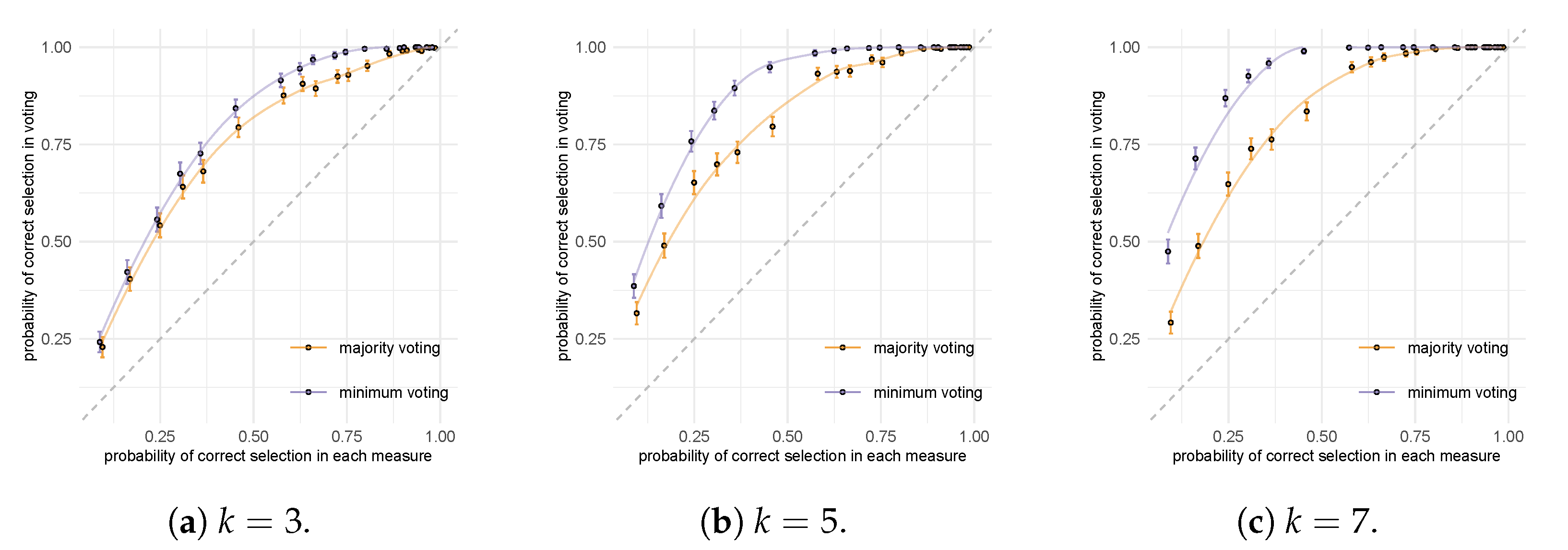
3.2. Inspirations of Minimum Voting

The idea of minimum voting originates from the hybrid NQS in Ref. [13], where NQS was implemented on k quantum nodes and the output state was chosen as the majority voting among all k states. However, when k is small, the diversified outcomes and ties can hamper the voting to reach a majority. Furthermore, the probability of an event in which the majority voting result selects the correct subset varies depending on the probability of selecting not only the solution states but also other possible states in D . In other words, with a fixed probability p of correct selection in each measurement, if a few non-solution states have a comparably high probability of being selected as the solution states, the probability of correct selection in majority voting would be much smaller than in the case where all non-solution states have approximately the same probability of being selected. In fact, majority voting does not perform well enough in the NQS mechanism, since all states with relatively small loss have a considerable probability of being selected unless the number of iterations is quite large. Consequently, the corresponding states would confuse the majority voting results. Estimating the likelihood of the event where the majority voting chooses the appropriate subset, represented as E , is a complex task. The subsequent theorem offers a lower limit on the successful probability associated with majority voting.
Theorem 1.
Assume every node operates independently in a quantum-classical network that comprises k = 2 s + 1 quantum nodes with a probability p > s + 1 2 s + 1 of choosing the accurate solution state. Let A represent the event where the majority vote of the output leans towards the right solution state. The probability of A to occur is then bounded below by
P ( A ) Φ 2 ( s + 1 ) D K L ( p , s + 1 2 s + 1 ) ,
where Φ ( · ) is the standard Gaussian cumulative distribution function and
D K L ( u , v ) = u ln u v + ( 1 u ) ln ( 1 u ) ( 1 v )
is the Kullback–Leibler divergence between two Bernoulli distributions with parameters u and v.
Compared with majority voting, choosing the state with the smallest loss function value over the k states undoubtedly increases the accuracy, with an extra small computational cost of order O ( k ) . With the same setup, i.e., k nodes and each node has a success probability p, the success probability of minimum voting admits
P ( A * ) = 1 ( 1 p ) k = 1 ( 1 p ) ( 2 ξ + 1 ) .
As we can see, P ( A * ) P ( A ) since the occurrence of A indicates that the solution state has been selected in the k measurements, and, consequently, A * occurs, i.e., A A * .
The aforementioned modification merely considers replacing the one-time majority voting in hybrid NQS with minimum voting. In contrast, RNQS incorporates minimum voting in every iteration, which not only outperforms hybrid NQS in terms of accuracy but also greatly accelerates the search process. The empirical advantage of minimum voting over majority voting is demonstrated through an experiment in Section 4.1.

4. Experiments

In this section, we conduct numerical experiments to validate some key ideas in this paper. We first compare the performances of minimum voting and majority voting in a quantum search mechanism. Second, we compare the empirical performance of NQS and RNQS in terms of their accuracy, computational cost, and robustness.

4.1. Minimum Voting versus Majority Voting

To obtain a clear comparison between minimum voting and majority voting in the quantum search regime, we evaluate the performance of hybrid NQS (i.e., NQS combined with majority voting or minimum voting) and NQS with minimum voting. For both methods, we set the number of quantum nodes to be k = 3 , 5, and 7. The dataset is generated as a random permutation of the integers from 0 to 31. Thus, we know that 0 is the minimum among the 32 numbers, but its location within the set is unknown. For both methods, we run 1000 replications. We calculate the probability of selecting 0 and the corresponding 95 % confidence interval after each iteration for both methods. Furthermore, we use 10 , 000 replications of NQS to approximate the baseline: the probability distribution of 32 states after each iteration without applying either majority or minimum voting. The results are reported in Figure 2.
The results demonstrate that both majority voting and minimum voting can enhance the success probability compared to the baseline. Furthermore, minimum voting consistently outperforms majority voting, which aligns with our discussion in Section 3.2. The advantage of minimum voting over majority voting is more pronounced when the success probability of a single node (i.e., the baseline) is low. This finding validates our conjecture that minimum voting is a superior strategy, as it not only improves accuracy but also strengthens robustness for quantum search.

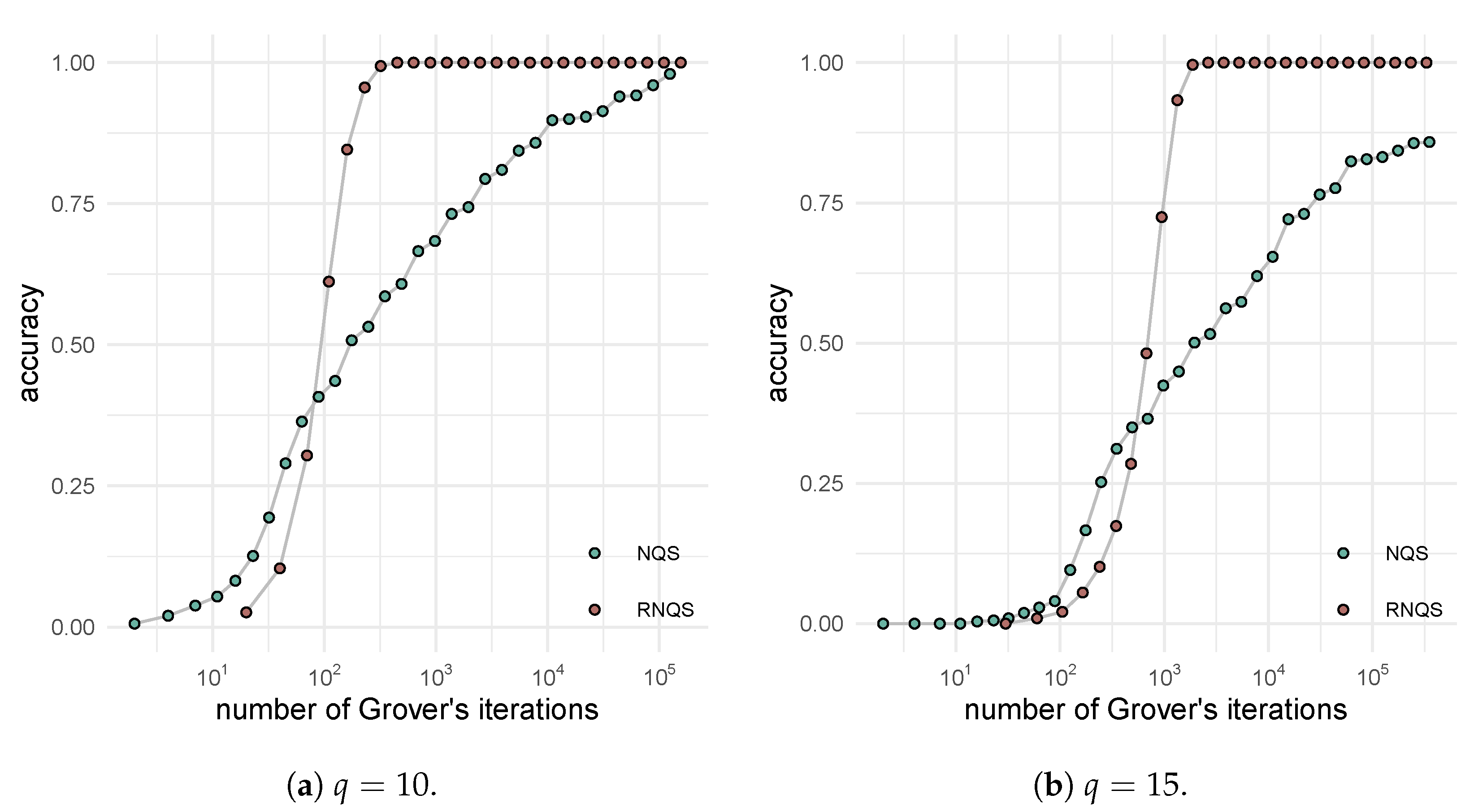
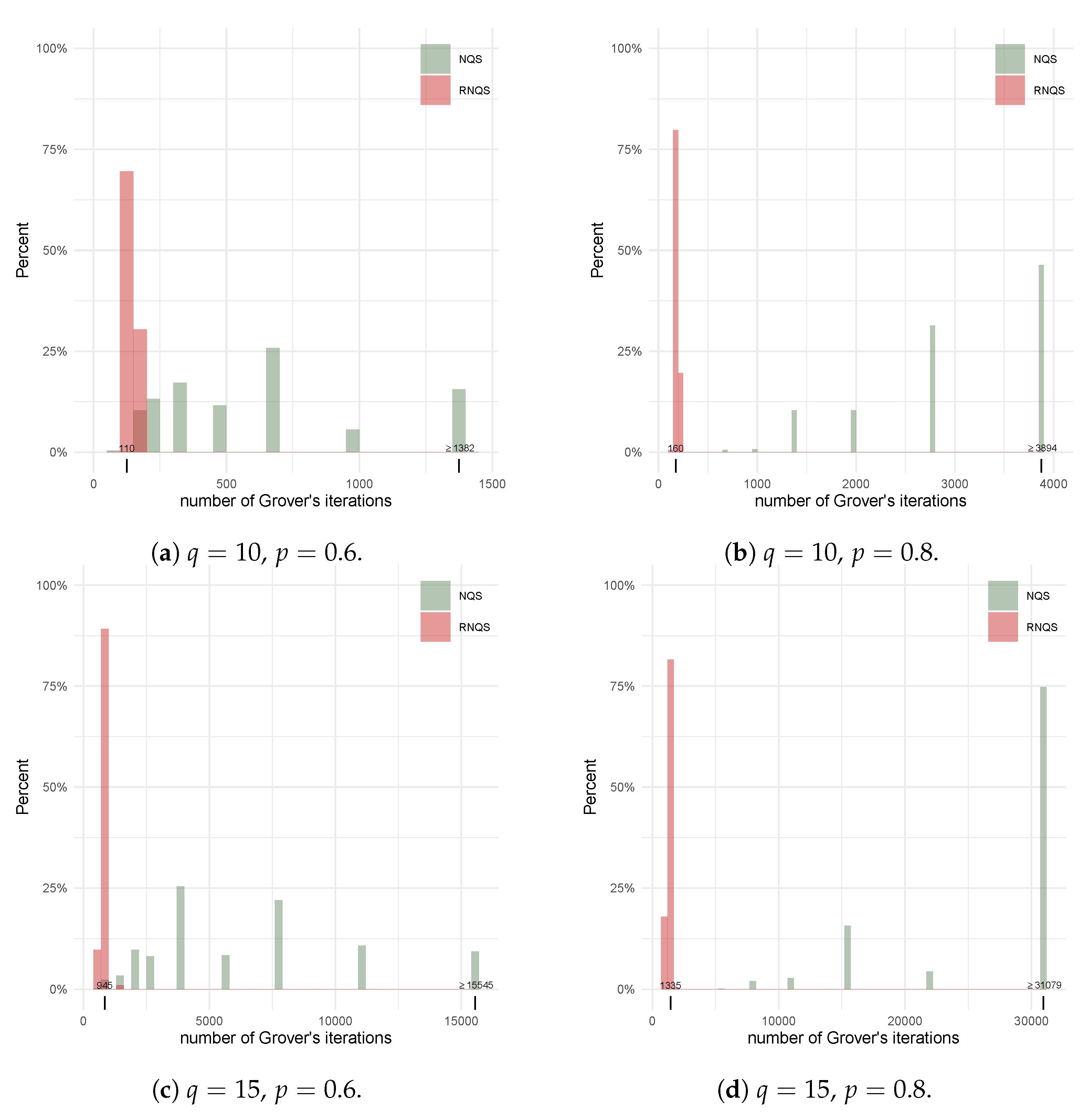
4.2. RNQS versus NQS: Accuracy and Computational Cost

In the second experiment, we compared the accuracy and computational cost of RNQS and NQS by applying them to search for the minimum in a random set of size D = 2 q for q = 10 and 15. The elements in the random set were drawn as a random permutation of the integers 0 , 1 , , 2 q 1 . For each method, we ran 500 replications and reported their accuracy probability versus the computational cost, measured by the total number of Grover’s operations used. The results are visualized in Figure 3. The comparison clearly shows that the accuracy probability of RNQS converges quickly to 1 within a few hundred Grover’s operations, while the accuracy probability of NQS requires more than 10 5 Grover’s operations to approach 1. Additionally, we observed that the computational cost of RNQS increases much more slowly with q compared to NQS. This experiment clearly justifies our conjecture that RNQS is a preferred alternative to NQS, as it significantly increases accuracy and reduces the computational cost.

4.3. RNQS versus NQS: Robustness Analysis

The third experiment was designed to compare the robustness of RNQS and NQS. We set q = 10 , 15, and 20. For each q, we established two desired accuracy probabilities, p = 0.6 and p = 0.8 . We repeated 500 replications for each scenario. In each replication, we recorded the number of Grover’s iterations needed by each method to achieve the desired accuracy probabilities. The empirical distribution of the recorded numbers provided us with key information to understand the robustness of RNQS and NQS. To that end, we reported the empirical quantiles of the recorded numbers in Table 1 and depicted histograms in Figure 4. As NQS converges too slowly, we only reported the results of RNQS for q = 20 .
The distributions of NQS are right-skewed and fat-tailed in all four cases. As a result, there is a non-negligible probability that NQS may fail to find the solution even with a huge number of Grover’s operations. This indicates that, if the user is not fortunate, NQS cannot successfully find the solution within a reasonable computational budget. This provides empirical evidence of the robustness concerns of NQS, as discussed in Section 2.3. On the other hand, the distributions of RNQS are tightly concentrated towards a very small sample median in all scenarios. Even for q = 20 (i.e., D = 2 20 = 1 , 048 , 576 ), the 95% quantile of RNQS is less than 10 thousand Grover’s operations and only less than 50% larger than its 5% quantile. The histograms in Figure 4 also provide a clear visual comparison between the empirical distributions of RNQS and NQS. The experimental results show strong evidence that RNQS is empirically robust and much more efficient than NQS.

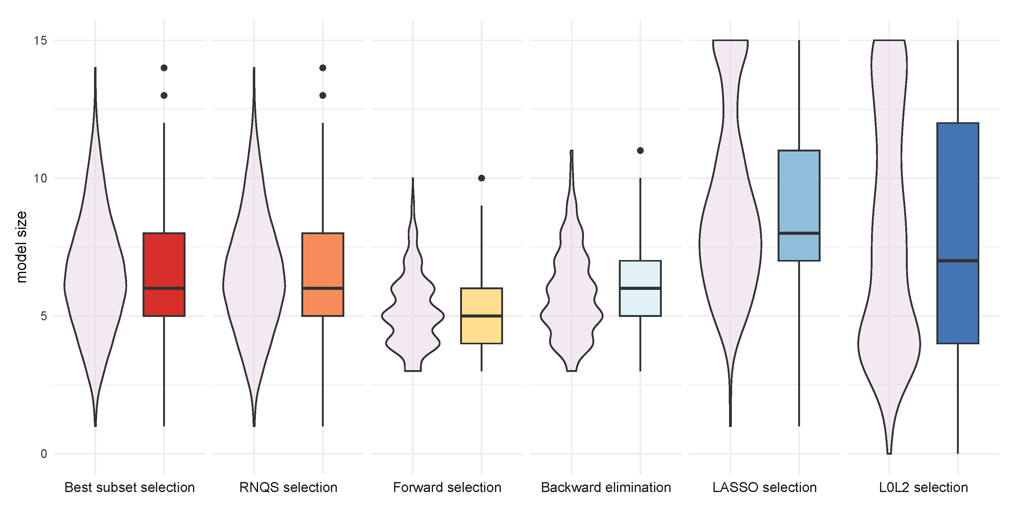
4.4. Application to Best Subset Selection for High-Dimension Linear Regression

Over the past few decades, numerous techniques have been proposed to address feature selection problems. Best subset selection, with a rich history dating back to Refs. [16,17], is notable. However, this approach is NP-hard, which led to the advent of Forward selection and Backward elimination techniques as proposed in Ref. [18] to counteract this complexity. While these methods can be effective, they may also be sensitive to factors like sample size and correlation among variables. Such sensitivities can make them unreliable or inconsistent in certain scenarios. The LASSO method, introduced in Ref. [19], emerged as a promising contender for producing sparse solutions. Nevertheless, LASSO has its shortcomings, particularly when managing highly correlated variables. It tends to retain just one variable and sets coefficients of other correlated variables to zero. This can pose challenges in high-dimensional datasets with prevalent correlations, even if the correlations are not pronounced at the population level. More recently, the methods proposed in Ref. [20] harness the power of coordinate descent and local combinatorial optimization for feature selection. As quantum computing continues to make strides, the RNQS algorithm offers a tantalizing opportunity to enhance Best subset selection for such problems.
In this application, we delve into a feature selection problem in the context of a linear additive model. Given a response vector Y, we aim to select features among p = 15 variables X 1 , , X 15 within a linear regression framework. With a sample size set at 100, the true model is represented by Y = 2 + 5 X 3 + 3 X 6 + 4 X 9 + 6 X 12 + 10 ϵ , wherein the covariate vector X = ( X 1 , , X 15 ) originate from a multivariate normal distribution with a mean of 0 . The power decay covariance matrix is given by Σ = ( σ i j ) 15 × 15 , where σ i i = 1 and σ i j = ρ | i j | for i j . In this scenario, ϵ N ( 0 , 1 ) is independent of X , and ρ is set at 0.8. Figure 5 showcases selected model sizes via box plots and violin plots for six distinct methods: Best subset selection, RNQS selection, Forward selection, Backward elimination, LASSO, and the 02 selection as presented in Ref. [20]. Despite each method’s intrinsic strengths and limitations, RNQS exemplifies the most faithful replication of Best subset selection. By capitalizing on the computational prowess of the RNQS algorithm, it becomes clear that the domain of 0 optimization in statistics and machine learning stands to benefit immensely.

5. Conclusions

The practical application of Grover’s Algorithm [15] is constrained, in part, by the necessity of oracle information, specifically the function S ( · ) in Algorithm 1. While NQS [13] was introduced to address this issue, it struggles to converge for large-scale problems and lacks robustness. In this paper, we propose a novel quantum algorithm that leverages multiple quantum nodes and incorporates the concept of minimum voting to enhance the precision and robustness of quantum search. Three simulation studies underscore the algorithm’s superior practical performance compared to its predecessor, NQS. Another simulation investigates the algorithm’s suitability for Best subset selection. Future research will explore the application of this algorithm in various additional statistical and machine learning problems involving 0 optimization, including sparse principal component analysis and Best subset selection.

Author Contributions

Conceptualization, Y.K.; methodology, T.Z. and Y.K.; software, T.Z.; validation, T.Z. and Y.K.; formal analysis, T.Z. and Y.K.; investigation, T.Z. and Y.K.; resources, Y.K.; data curation, T.Z.; writing—original draft preparation, T.Z.; writing—review and editing, Y.K.; visualization, T.Z.; supervision, Y.K.; project administration, Y.K.; funding acquisition, Y.K. All authors have read and agreed to the published version of the manuscript.

Funding

This research is supported by the National Science Foundation grant number NSF-2210468, NSF-2324389, and NSF-2243044, and the National Institute of Health grant number NIH-1R01HL172291.

Institutional Review Board Statement

Not applicable.

Informed Consent Statement

Not applicable.

Data Availability Statement

The data presented in this study are available on request from the corresponding author.

Conflicts of Interest

The authors declare no conflict of interest. The funders had no role in the design of the study; in the collection, analyses, or interpretation of data; in the writing of the manuscript; or in the decision to publish the results.

Abbreviations

The following abbreviations are used in this manuscript:
NQSNon-oracular Quantum Search
RNQSRobust Non-oracular Quantum Search

References

  1. Nielsen, M.A.; Chuang, I.L. Quantum Computation and Quantum Information; Cambridge University Press: Cambridge, UK, 2010. [Google Scholar]
  2. Jin, C.; Jin, S.W. Prediction approach of software fault-proneness based on hybrid artificial neural network and quantum particle swarm optimization. Appl. Soft Comput. 2015, 35, 717–725. [Google Scholar] [CrossRef]
  3. Zhou, N.R.; Xia, S.H.; Ma, Y.; Zhang, Y. Quantum particle swarm optimization algorithm with the truncated mean stabilization strategy. Quantum Inf. Process. 2022, 21, 42. [Google Scholar] [CrossRef]
  4. Zhou, N.R.; Zhang, T.F.; Xie, X.W.; Wu, J.Y. Hybrid quantum–classical generative adversarial networks for image generation via learning discrete distribution. Signal Process. Image Commun. 2023, 110, 116891. [Google Scholar] [CrossRef]
  5. Grover, L.K. Quantum mechanics helps in searching for a needle in a haystack. Phys. Rev. Lett. 1997, 79, 325. [Google Scholar] [CrossRef]
  6. Boyer, M.; Brassard, G.; Høyer, P.; Tapp, A. Tight bounds on quantum searching. Fortschritte Der Phys. Prog. Phys. 1998, 46, 493–505. [Google Scholar] [CrossRef]
  7. Kwiat, P.; Mitchell, J.; Schwindt, P.; White, A. Grover’s search algorithm: An optical approach. J. Mod. Opt. 2000, 47, 257–266. [Google Scholar] [CrossRef]
  8. Long, G.L. Grover algorithm with zero theoretical failure rate. Phys. Rev. A 2001, 64, 022307. [Google Scholar] [CrossRef]
  9. Høyer, P.; Neerbek, J.; Shi, Y. Quantum complexities of ordered searching, sorting, and element distinctness. Algorithmica 2002, 34, 429–448. [Google Scholar]
  10. Biham, E.; Biham, O.; Biron, D.; Grassl, M.; Lidar, D.A. Grover’s quantum search algorithm for an arbitrary initial amplitude distribution. Phys. Rev. A 1999, 60, 2742–2745. [Google Scholar] [CrossRef]
  11. Biham, E.; Kenigsberg, D. Grover’s quantum search algorithm for an arbitrary initial mixed state. Phys. Rev. A 2002, 66, 062301. [Google Scholar] [CrossRef]
  12. Brassard, G.; Høyer, P.; Mosca, M.; Tapp, A. Quantum Amplitude Amplification and Estimation. arXiv 2000, arXiv:quant-ph/0005055. [Google Scholar]
  13. Chen, J.; Park, C.; Ke, Y. Learning High Dimensional Multi-response Linear Models with Non-oracular Quantum Search. In Proceedings of the 2022 IEEE International Conference on Quantum Computing and Engineering (QCE), Broomfield, CO, USA, 18–23 September 2022; pp. 1–12. [Google Scholar] [CrossRef]
  14. Bennett, C.H.; Bernstein, E.; Brassard, G.; Vazirani, U. Strengths and weaknesses of quantum computing. SIAM J. Comput. 1997, 26, 1510–1523. [Google Scholar] [CrossRef]
  15. Grover, L.K. A fast quantum mechanical algorithm for database search. In Proceedings of the Twenty-Eighth Annual ACM Symposium on Theory of Computing, Philadelphia, PA, USA, 22–24 May 1996; ACM: New York, NY, USA, 1996; pp. 212–219. [Google Scholar]
  16. Beale, E.; Kendall, M.; Mann, D. The discarding of variables in multivariate analysis. Biometrika 1967, 54, 357–366. [Google Scholar] [CrossRef] [PubMed]
  17. Hocking, R.; Leslie, R. Selection of the best subset in regression analysis. Technometrics 1967, 9, 531–540. [Google Scholar] [CrossRef]
  18. Efroymson, M. Stepwise regression—A backward and forward look. In Proceedings of the Eastern Regional Meetings of the Institute of Mathematical Statistics, Long Island, NY, USA, 27–29 April 1966; pp. 27–29. [Google Scholar]
  19. Tibshirani, R. Regression shrinkage and selection via the lasso. J. R. Stat. Soc. Ser. B 1996, 58, 267–288. [Google Scholar] [CrossRef]
  20. Hazimeh, H.; Mazumder, R. Fast best subset selection: Coordinate descent and local combinatorial optimization algorithms. Oper. Res. 2020, 68, 1517–1537. [Google Scholar] [CrossRef]
Figure 1. An illustrative example ( D = 2 5 = 32 ) for Robust Non-oracular Quantum Search. The subfigures represent the absolute amplitude of states in various superpositions within the algorithm.
Technologies 11 00148 g001
Figure 2. Probability of correct selection in majority/minimum voting versus the probability of correct selection in each measure for quantum search with 5 qubits. Three patterns are plotted for different k values. Over 1000 replications, the calculated probabilities are illustrated as dots, while their associated 95% confidence intervals are depicted using vertical error bars. The unbroken lines present the smoothed trajectories. The dashed lines on the diagonal are references for probability of correct selection in each measure.
Technologies 11 00148 g002
Figure 3. Increment of accuracy in number of Grover’s operations for NQS and RNQS.
Technologies 11 00148 g003
Figure 4. Histograms of number of Grover’s operations to achieve specific accuracy p.
Technologies 11 00148 g004
Figure 5. Violin plots and Box plots of the selected model size. Six patterns are plotted for different methods. In each box plot, the bold line represents the median; two hinges represent the 25% and 75% quantile; the length of the whiskers is 1.5 of IQR.
Technologies 11 00148 g005
Table 1. Simulation results over 500 replications showing quantiles of N G .
AccuracyAlgorithmNQSRNQS
Quantile5%10%25%50%75%90%95%5%10%25%50%75%90%95%
p = 0.6 q = 10 17617634949269413821382110110110110160160160
q = 15 1382195138945503777810,99515,545675945945945945945945
q = 20 -------4960496049606980698069806980
p = 0.8 q = 10 13821382275627565503777810,995160160160160160230230
q = 15 15,317.515,54521,97943,947≥62,146≥62,146≥62,14694594513351335133513351335
q = 20 -------6980698069806980984098409840
Disclaimer/Publisher’s Note: The statements, opinions and data contained in all publications are solely those of the individual author(s) and contributor(s) and not of MDPI and/or the editor(s). MDPI and/or the editor(s) disclaim responsibility for any injury to people or property resulting from any ideas, methods, instructions or products referred to in the content.

