Article

Image Denoising Using Hybrid Deep Learning Approach and Self-Improved Orca Predation Algorithm

by
Rusul Sabah Jebur
1,*,
Mohd Hazli Bin Mohamed Zabil
2,
Dalal Abdulmohsin Hammood
3,
Lim Kok Cheng
2 and
Ali Al-Naji
3,4,*
1
Faculty of Information and Communication Technology, University Tenaga National, Kajang 43000, Malaysia
2
Department of Computing, College of Computing and Informatics, Universiti Tenaga National, Kajang 43000, Malaysia
3
Electrical Engineering Technical College, Middle Technical University, Baghdad 10022, Iraq
4
School of Engineering, University of South Australia, Mawson Lakes, SA 5095, Australia
*
Authors to whom correspondence should be addressed.
Technologies 2023, 11(4), 111; https://doi.org/10.3390/technologies11040111
Submission received: 4 July 2023 / Revised: 3 August 2023 / Accepted: 8 August 2023 / Published: 12 August 2023

Abstract

:
Image denoising is a critical task in computer vision aimed at removing unwanted noise from images, which can degrade image quality and affect visual details. This study proposes a novel approach that combines deep hybrid learning with the Self-Improved Orca Predation Algorithm (SI-OPA) for image denoising. Leveraging Bidirectional Long Short-Term Memory (Bi-LSTM) and optimized Convolutional Neural Networks (CNN), the hybrid model aims to enhance denoising performance. The CNN’s weights are optimized using SI-OPA, resulting in improved denoising accuracy. Extensive comparisons against state-of-the-art denoising methods, including traditional algorithms and deep learning-based techniques, are conducted, focusing on denoising effectiveness, computational efficiency, and preservation of image details. The proposed approach demonstrates superior performance in all aspects, highlighting its potential as a promising solution for image-denoising tasks. Implemented in Python, the hybrid model showcases the benefits of combining Bi-LSTM, optimized CNN, and SI-OPA for advanced image-denoising applications.

1. Introduction

The goal of image denoising, a crucial task in image processing and computer vision, is to eliminate the noise that is frequently added to images during image collecting, transmission, or processing. Noise can degrade image quality, impair the precision of image-based analysis, and negatively impact how well activities like object recognition, segmentation, and tracking function later on [1,2]. As a result, image denoising has garnered a lot of research attention over the years, leading to the development of several techniques to solve it. But conventional image denoising techniques, like Masked Joint Bilateral Filtering (MJBF) and CT- image based Generative adversarial network (CT-GAN) approaches, frequently have several drawbacks, including high computational complexity, poor adaptability to various noise types and levels, and difficulty preserving image details and textures [3,4]. Deep learning-based methods have recently come to light as a potential approach to image denoising, generating cutting-edge results in terms of both quantitative measures and visual quality. The success of deep learning-based denoising can be due to its capacity to acquire sophisticated image features and high-level representations directly from the training data without depending on explicit handcrafted features or presumptions on the noise distribution [5,6,7]. Deep learning models also enable joint optimization of the denoising method and the image representation because they may be trained from beginning to end. Discriminative and generative models are two main categories that can be used to classify deep learning-based image-denoising techniques.
CNN, among other discriminative models, can directly transfer noisy images to the equivalent clean versions [8,9]. The purpose of training these models is to reduce the reconstruction error between the predicted and ground-truth images. Typically, pairs of clean and noisy images are used, and each pair is used to train a different model. On many datasets, including BSD68, Set12, and Kodak24, CNN-based denoising techniques have demonstrated outstanding performance, surpassing more established denoising techniques by a significant margin. Additionally, CNN-based electrical noise removable models can be denoised optoacoustic tomography data by significantly improving the data quality of using multispectral optoacoustic tomography (MSOT). As well as, similarity informed self learning (SISL) is proposed to remove seismic image, trained unsupervised or semi-supervised, minimizing the need for annotated training data. While generative models, on the other hand, the sample from the distribution of clean and noisy images based on the observed noisy image, they seek to learn the underlying probability distribution of both types of images [10,11,12]. The variational autoencoder (VAE), a kind of deep generative model that learns a latent representation of an image and a decoder that maps this representation to a clean image, is the most widely used generative model for image denoising. In several applications, including MRI denoising, video denoising, and low-dose CT imaging, VAE-based denoising techniques have demonstrated promising results. Additionally, VAE-based algorithms can produce numerous believable denoised images by sampling from the learned distribution, which can be helpful for downstream tasks like uncertainty assessment. Additional, theoretically-grounded blind and universal deep learning to revmove additive guassion noise called Blind Universal Image Fusion Denoiser (BUIFD), complex value convolutional neural network (CDNet). In CDNet. Nueral network (NN) suffer from possible instability of back propagation computational issues for gradient-descend-based training, so, it is better to design activiation function. As well as, amulti stage image denoising CNN with the wavelet transform (MWDCNN) is suggested to reduce noise [13,14,15,16].
Other deep learning architectures, in addition to CNNs, have also been investigated for image denoising [17], including recurrent neural networks (RNNs), generative adversarial networks (GANs), and attention-based models. The performance of RNN-based denoising techniques is enhanced by using the temporal correlations between neighboring frames in video sequences. The GAN-based denoising methods encourage the generated images to be indistinguishable from the clean images by introducing an adversarial loss to the denoising objective [18]. The efficiency and effectiveness of the denoising process can be increased by using attention-based models to preferentially focus on the most informative image regions and features [19,20]. Deep learning-based denoising techniques have been successful, but there are still several issues that need to be resolved.
Present Proposed Work:
  • Approach: Hybrid deep learning combining Bi-LSTM and optimized CNN.
  • Objective: Improve image denoising performance.
  • Bi-LSTM captures temporal dependencies, while the optimized CNN focuses on spatial features.
  • CNN weights are optimized using SI-OPA, a nature-inspired algorithm mimicking orca hunting behavior.
  • Extensive comparisons against state-of-the-art methods.
Previous Existing Works:
  • Various image denoising methods: traditional algorithms and deep learning-based techniques.
  • Approach: Diverse algorithms with different denoising strategies.
  • Evaluation: Various performance metrics and visual assessments.
  • Baseline for comparison against the proposed hybrid approach.
The major contribution of this research work is as follows:
  • A hybrid deep learning approach is proposed, combining Bi-LSTM and an optimized CNN, for the task of image denoising. Bi-LSTM is utilized to capture temporal dependencies in the image data, while the optimized CNN focuses on extracting spatial features. This combination aims to leverage the strengths of both architectures for improved denoising performance.
  • The weights of the CNN model are optimized using SI-OPA. OPA is a nature-inspired optimization algorithm that mimics the hunting behavior of orcas. By applying OPA to the CNN training process, the algorithm aims to enhance the performance and convergence of the network. The OPA algorithm adapts the positions of the orcas, representing the CNN weights, based on a fitness function that evaluates the denoising performance.
  • The performance of the proposed approach is compared against state-of-the-art image denoising methods. Various existing methods for image denoising, including traditional algorithms and deep learning-based techniques, are considered baselines. Through comprehensive evaluation metrics and visual assessments, the proposed hybrid approach is assessed in terms of denoising effectiveness, computational efficiency, and its ability to preserve image details and textures. The comparison aims to highlight the advantages and improvements offered by the proposed approach over existing methods.
The subsequent sections of this paper are organized as follows: Section 2 provides an overview of the literature reviews related to the subject matter. Section 3 presents the proposed methodology. Section 4 presents the documented results of the study. Finally, Section 5 concludes this paper.

2. Literature Review

In recent years, significant progress has been made in the field of image denoising, driven by advancements in deep learning techniques. This literature review explores several notable studies published between 2019 and 2022, which introduce innovative approaches for denoising different types of images as follows:
In 2019, Dong et al. [21] used a novel deep-learning framework for 3-D hyperspectral image (HSI) denoising, which encodes rich multi-scale information using a modified 3-D U-net. The approach is computationally efficient and achieves substantial savings on the number of network parameters by using a separable filtering strategy. Transfer learning is also used to generate synthetic HSI data for initial training, which outperforms existing model-based HSI denoising methods according to experimental results.
Another study by Hashimoto et al. (2019) [22] developed a DIP approach for dynamic PET image denoising, which does not require pre-training or large datasets. Static PET data are used as input, while dynamic PET images are used as training labels. The proposed method is applied to both computer simulations and real data and produces less noisy and more accurate images than other algorithms. The DIP method is found to perform better than other post-denoising methods in terms of contrast-to-noise ratio and can be applied to low-dose PET imaging.
Another study by Kokkinos and Lefkimmiatis (2019) [23] proposed a novel algorithm for joint image demosaicking and denoising using a trainable residual denoising network. Our approach is inspired by classical image regularization methods, large-scale optimization, and deep learning techniques. The derived iterative optimization algorithm outperforms previous approaches for both noisy and noise-free data across different datasets and requires fewer trainable parameters than the current state-of-the-art solution.
In 2020, Liu et al. [24] proposed a joint approach to image denoising and high-level vision tasks using deep learning, exploring how they can influence each other. The proposed method includes a Convolutional Neural Network that fuses contextual information on different scales and a deep neural network solution that cascades two modules for image denoising and high-level tasks, respectively. Experimental results show that the approach can overcome performance degradation and produce visually appealing results with guidance from high-level vision information.
A study by Wu et al. (2021) [25] used a self-supervised deep-learning method for denoising dynamic computed tomography perfusion (CTP) images without requiring high-dose reference images for training. The proposed method maps each frame of CTP to an estimation from its adjacent frames, effectively removing noise due to independent noise in the source and target. The method achieves improved image quality, spatial resolution, and contrast-to-noise ratio compared to conventional denoising methods and supervised learning approaches.
Li et al. (2021) [26] developed deep neural network (DNN)-based image denoising methods on binary signal detection tasks in medical imaging. Traditional image quality measures are not sufficient for evaluating DNN-based denoising methods. The study uses task-based IQ measures to evaluate the performance of DNN-based denoising methods on binary signal detection tasks. The results suggest the need for objective evaluation of IQ for DNN-based denoising technologies to improve their effectiveness in medical imaging applications.
Another study by Ma et al. (2022) [27] introduced a new deep network architecture, called DBDnet, for image denoising. The network generates a noise map and gradually updates it using a boosting function. The denoising process is framed as reducing the noise of the noise map (NoN), and the proposed method includes a non-eliminating module to simulate this process.
Chen et al. (2022) [28] used a novel denoising framework, TEMDnet, for the transient electromagnetic method (TEM) signal denoising task. The existing DNN methods for TEM denoising are not flexible enough to deal with various signal scales. TEMDnet transforms the signal-denoising task into an image-denoising task by using a novel signal-to-image transformation method and a deep CNN-based denoiser with a residual learning mechanism. The proposed framework achieves better performance than traditional methods and is more flexible for various signal scales.
Bahnemiri et al. (2022) [29] proposed a deep learning method for estimating the map of local standard deviations of noise (sigma-map) to improve image denoising performance in the case of non-stationary noise. The method achieves state-of-the-art accuracy in estimating sigma maps and outperforms recent CNN-based blind denoising methods by up to 6 dB in PSNR. It also provides better usage flexibility compared to other state-of-the-art sigma-map estimation methods. The proposed method shows a small difference in PSNR values compared to the ideal case when a ground-truth sigma map is available.
Wang et al. (2022) [30] developed a new denoising method for hyperspectral images combining traditional machine learning and deep learning techniques. The method, called NL-3DCNN, exploits the high spectral correlation of an HSI using subspace representation and groups non-local similar patches for denoising using a 3-D Convolutional Neural Network. Experimental results show that the proposed method outperforms state-of-the-art methods for both simulated and real data.
In the realm of image denoising, conventional methods have faced limitations when dealing with complex and noisy environments, particularly in the case of salt and pepper noise. While deep learning techniques have displayed significant success in this domain, there is still a pressing need to further improve noise reduction without compromising image quality. Numerous image-denoising approaches, encompassing statistical, filtering-based, and deep learning-based methods, have been proposed. Nevertheless, achieving high-quality denoising outcomes continues to be a challenging task [1,8]. To address this issue, this research puts forth a hybrid deep learning strategy that combines Bi-LSTM with CNN. By coordinating the strengths of both models, this approach aims to attain superior image-denoising results. Moreover, to further boost performance and overcome the existing limitations in image denoising, the Self-Improved Orca Predation Algorithm (OPA) is utilized to optimize the weights of the CNN. This adaptive optimization process aims to enhance the denoising capabilities of the CNN, specifically targeting salt and pepper noise reduction. By fusing the power of Bi-LSTM and Optimized CNN with the adaptive capabilities of OPA, this research seeks to achieve a novel and efficient solution for high-quality image denoising in challenging and noisy environments. The proposed approach has the potential to advance the field of image processing, offering improved denoising results and finding applications in various domains such as medical imaging, surveillance, and image. Table 1 shows the research gaps.

3. Proposed Methodology

Image denoising is a crucial task in various applications like medical image analysis, remote sensing, and computer vision. Traditional methods have limitations in complex and noisy environments. Deep learning has achieved remarkable success, but further improvements are needed. This research developed a hybrid approach combining Bi-LSTM and optimized CNN to enhance image-denoising results. The weights of the CNN are optimized using the Self-Improved Orca Predation Algorithm (SI-OPA) algorithm to reduce noise while maintaining image quality.
Step 1: Data Collection: The first step in the proposed methodology for image denoising using deep learning with a hybrid Bi-LSTM and optimized CNN is data collection. In this step, Gaussian noise is added to the collected input data.
Step 2: Denoising: A new hybrid deep learning model is introduced for image denoising. This model combined Bi-LSTM and optimized CNN to improve denoising results. The weights of the CNN are optimized using the Self-Improved Orca Predation Algorithm (SI-OPA), which is an efficient optimization algorithm inspired by the hunting behavior of Orcas. The SI-OPA aims to enhance the performance of the CNN by optimizing its weights.
Step 3: Evaluation: The proposed hybrid deep learning model can be evaluated using metrics such as Peak Signal-to-Noise Ratio (PSNR) and Structural Similarity Index (SSIM) to assess its performance in image processing tasks. These metrics are commonly used to measure the quality and similarity between the reconstructed or enhanced images and their original versions. The overall architecture diagram is shown in Figure 1.

3.1. Data Collection

Adding Gaussian noise to collected input data is a common technique used to simulate noisy environments or to test the robustness of models against noise. Gaussian noise follows a Gaussian distribution and can introduce random variations to the data. By adding Gaussian noise to the input data, it is possible to evaluate the performance of the proposed approach (hybrid deep learning model) under noisy conditions. When evaluating the model’s performance with Gaussian noise, it is important to consider how the noise affects the output and compare it to the original data. Metrics such as PSNR and SSIM can still be used to assess the quality and similarity of the reconstructed or enhanced images, even in the presence of added Gaussian noise. These metrics can provide insights into how well the model can handle noise and preserve the important features of the data. Adding Gaussian noise to collected input data can help assess the robustness and performance of the proposed hybrid deep learning model in the presence of noise.

3.1.1. Pre-Processing

In this research work, preprocessing is performed using Gaussian Filtering to remove noise, correcting intensity inhomogeneity via histogram equalization and skull stripping.

3.1.2. Skull Stripping

The collected raw MRI images are fed as input to skull stripping. Skull stripping is a pre-processing step commonly used in medical image analysis to remove the non-brain tissues, such as the scalp, skull, and meninges, from the brain MRI images. It is essential for intensity inhomogeneity correction, which aims to address the problem of varying signal intensities in different regions of the image due to the differences in magnetic field strengths, acquisition protocols, and hardware variations. Intensity inhomogeneity in MRI images can cause a significant problem in the segmentation and registration of brain images as it affects the accuracy and reliability of these procedures. Skull stripping helps to reduce intensity inhomogeneity by removing non-brain tissues that may cause signal variations. The removal of non-brain tissues also reduces the computational burden and processing time required for segmentation and registration algorithms. Model-based and atlas-based skull stripping procedures can be divided into two major categories. Model-based approaches rely on statistical models that describe how the brain and non-brain tissues are shaped and appear. Atlas-based methods involve registering a pre-labeled atlas brain image to the patient’s image and using the resulting transformation to remove the non-brain tissues. Gaussian filtering is employed on skull-stripped images.

3.1.3. Gaussian Filtering

In order to eliminate noise from an image, the Gaussian filtering technique is frequently utilized. It is used in the pre-processing step of AD early detection to reduce noise in MRI images. The method operates by convoluting the image using a bell-shaped-curve function called a Gaussian kernel. The degree of image smoothing is based on the size of the kernel. The image is made clearer and simpler to deal with by eliminating noise, which might increase the precision of the following steps in the pipeline for AD detection. The size of the kernel must be carefully set to balance noise reduction with retention of key visual features because excessive smoothing can also result in loss of clarity and information in the image. In the processing of multi-resolution images, Gaussian filters are frequently used. The image must typically be convolutional with numerous Gaussian filters of increasing spread in multi-resolution approaches. A finite impulse response method requires a lot of work to compute the convolution for large values of the spread because there are many filter coefficients involved. Pyramid techniques exploit the fact that a Gaussian function can be factorized into a convolution of Gaussian functions with a smaller spread as per Equation (1).
F ( σ ) = F ( σ , )   F ( σ 2 )   F ( σ M ) ,
where σ s σ and σ 2 = s = 1 M σ s 2 .
The saving in calculations is achieved by using fewer filter coefficients for each F ( σ s ) , since the spread σ s is smaller than σ , and by subsampling the image after each intermediate convolution F ( σ s ) , since each Gaussian filter F ( σ s ) reduces the bandwidth of the images. The intensity inhomogeneity correction is performed on the noise-free image using histogram equalization.

3.1.4. Histogram Equalization

Intensity inhomogeneity is a common problem in medical images, including MRI scans, where some parts of the image may appear darker or brighter than other areas. This can make it difficult to accurately detect and analyze features in the image, including abnormalities such as those associated with AD. Histogram equalization is a technique used to correct intensity inhomogeneity by enhancing the contrast of an image. This is performed by redistributing the intensity values of the image so that they are spread out more evenly across the available range. In other words, histogram equalization maps the original pixel values to new pixel values that have a more uniform distribution, resulting in a more balanced image that is easier to analyze. The histogram equalization process involves creating a histogram of the image, which shows the distribution of pixel values across the image. The histogram is then used to create a mapping function that adjusts the pixel values of the image to improve the contrast. This mapping function can be applied to the entire image or to specific regions of interest (ROIs) in the image. By applying histogram equalization to MRI images, the intensity inhomogeneity can be corrected, leading to improved accuracy in the detection of AD. After the pre-processing stage, the noise-free image with corrected intensity inhomogeneity is passed on to the segmentation phase. In this phase, the goal is to identify the region of interest (ROI) in the MRI image that contains the brain structures necessary for AD detection.

3.2. Denoising

Introducing a new hybrid deep learning model that combined Bi-LSTM and optimized CNN for image denoising sounds promising. By leveraging the strengths of both architectures, it is possible to enhance the denoising results and achieve better image quality. In this hybrid model, the Bi-LSTM component can capture long-term dependencies in the image data, allowing for more effective denoising. The Bi-LSTM can learn and preserve the contextual information in the image, which can aid in removing noise while retaining important image features. The optimized CNN plays a crucial role in the model by using SI-OPA to optimize its weights. SI-OPA, inspired by the hunting behavior of Orcas, is an optimization algorithm designed to enhance the performance of CNN. By optimizing the weights of the CNN using SI-OPA, the model can adaptively adjust its parameters to improve its denoising capabilities. The proposed hybrid deep learning model combining Bi-LSTM and optimized CNN shows promise for image denoising. By leveraging the strengths of both components and employing SI-OPA for weight optimization, the model aims to deliver improved denoising results and enhance the overall image quality.

3.3. Bi-LSTM

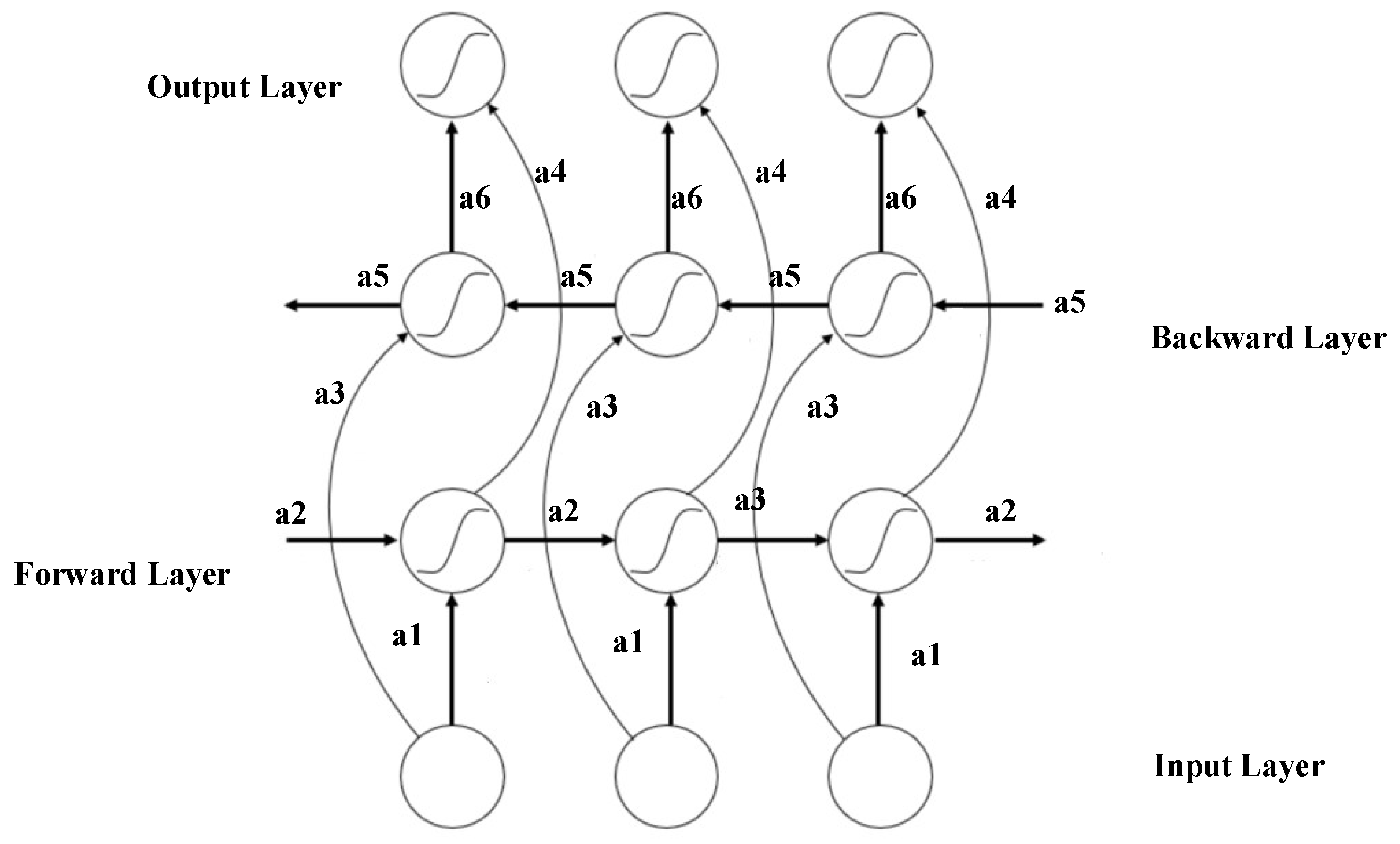
Networks are separately fed the retrieved horizontal and vertical spatial feature sequences to produce deep spatial–angular features. Each Bi-LSTM [31] network can be modeled as two separate conventional LSTM networks, one of which analyses the input sequence in the forward direction (left to right) and the other which analyses it in the backward direction. This allows each Bi-LSTM network to capture both forward and backward relationships within a sequence (right to left). The outputs of the Bi-LSTM network are then created by concatenating the hidden output states. The Bi-LSTM and its associated layers are illustrated in Figure 2.
Due to the recurrent connections between each unit, RNNs are effective in representing hidden sequential patterns of data. However, updating the network parameters during backpropagation is difficult because of the “vanishing gradient” problem and the RNN recurrent structure’s “internal memory” feature. RNNs are, therefore, inefficient at comprehending early information and replicating the long-term temporal contexts of feature vector sequences. Fortunately, LSTM avoids this fundamental issue because of its unique cell structure, which consists of forget, input, and output gates controlled by sigmoid units to decide what data to update and store in memory cells. Through linear connections, these LSTM units transmit the previous data to the current time step”. The processes inside the LSTM cell may be expressed as follows given the current input vector A t , the most recent hidden state h t 1 and the most recent memory cell state c t 1 as per Equations (2)–(7).
I n p t = S a ( I A . I n p A t + R h .   i n p h t 1 + b v ( i n p )
F g t = S a ( I A . F g A t + R h .   F g h t 1 + b v ( F g )
O u t t = S a ( I A . O u t A t + R h .   O u t h t 1 + b v ( O u t )
m t = B ( I A t A t + R h c h t 1 + b v ( c )
c t = F g t c t 1 + m t .   I n p t
h t = O u t t . B ( c t )
where I n p t , F g t , O u t t , and m t stand for the input, forget, output, and input modulation gates, respectively, at time t. Input weights, recursive weights, and bias vectors are denoted by the letters I A , R , and b v . The sigmoid activation function is represented by S a ( A ) = ( 1 + e A ) 1 , while the hyperbolic tangent function is represented by B ( A ) = ( e A e A ) / ( e A + e A ) . The tanh activation function derives. F g t is a vector that offers potential values to update the memory cell from the current input and the prior state. The memory cell’s contents are controlled by the input gates it and F g t , while the forget gate F g t v determines which previously communicated data should be discarded. The output gate O u t t stores the data for forthcoming operations that control the cell’s output at time t. The output gate vector O u t t and the current memory cell state O u t t , after being projected by the tanh function, may be multiplied element-wise to find the hidden state h t at time t. Afterward, the memory cell is designated as c t is updated. By stacking two LSTM layers in opposition to one another, we create a network that starts with the bidirectional temporal patterns of feature vector sequences. In contrast to the outputs of a typical single-layer LSTM at time t, the combined outputs of Bi-LSTM layers are influenced by signals from both past and future vectors. Bi-LSTM networks may thus build higher-level global context connections of sequential data from movies by including the additional information from future data. CNN feature vectors acquired from the encoder and organized in temporal sequences serve as the visual representation of each video clip. The temporal connections of the characteristics are written as per Equation (8).
D t = m ( F g t | D t 1 )
In this context, D t denotes the temporal data, F g t denotes the feature vectors modeled at time t, and m is the modeling function for temporal connections. Our study employed the Bi-LSTM network to separately abstract the temporal representation of the past and future data, which only takes into account the past data. The output of the LSTM was then created by combining two of its hidden states”, which is given as per Equation (9).
D t = m ( F g t | D t 1 , D t + 1 )

3.4. Optimized CNN

CNN [32], an Artificial Neural Network (ANN) based on deep learning theory, has been widely used in the field of object identification and prediction. Images with a 2D grid can automatically be processed using CNN to extract spatial characteristics. The activation function, pooling layer, fully connected layer, and convolutional layer make up the majority of CNN.
(a) 
Convolutional Layer
The convolution process in the convolutional layer, which is used to extract visual information and learn the map out between the input and output layers, replaces the matrix multiplication operation in the classic neural network. Sharing parameters during the convolution process allows the network to learn only one set of parameters, substantially lowering the number of parameters and improving computing performance. A convolution operation is described as per Equation (10).
v i , j = q = 0 C n = 0 C l q , n s k + q , b + n
where l q , n is the scale of the convolutional kernel. s k , b is the pixel value of the image at k and b .
(b) 
Activation Function
To avoid vanishing gradients and hasten training, CNN commonly uses rectified linear unit (ReLU) activation functions. The following is a description of ReLU’s goal. This is mathematically shown in Equation (11). The optimized CNN is illustrated in Figure 3.
R e L U ( r ) = { r     r > 0 0     r   0 .
(c) 
Pooling layer
The pooling layer can concentrate the details in feature maps while reducing the complexity of the computerized network. Max pooling is the common pooling layer. This is mathematically shown in Equation (12).
M a x P o o l ( e ,   m ) = { e = f l o o r ( ( e i + 2 p o ) c + 1 ) m = f l o o r ( ( m i + 2 p o ) c + 1 )  
where F l o o r ( S ) was the function of bringing together numbers, e is the output height of the feature map, and m is the output width of the feature map. e i is the intake height of feature maps, m i is the input breadth of feature maps, p is the padding of feature maps, o is the kernel size of max pooling, and c is the kernel stride of max pooling. Using SI-OPA, the weights of a CNN can be optimized to enhance its performance.

3.5. Self-Improved Orca Predation Algorithm (SI-OPA)

The Orca Optimization Algorithm [33] is a metaheuristic optimization algorithm inspired by the hunting behavior of killer whales (orcas) in nature. It mimics the hunting strategies of orcas to solve optimization problems. In the Orca Optimization Algorithm, a population of virtual orcas is initialized, and each orca represents a potential solution to the optimization problem. The orcas swim through the search space, simulating the exploration of potential solutions. The movement of orcas is guided by their individual and collective behaviors.

3.5.1. Driving Phase

In the driving phase of the OPA algorithm, recent advancements have introduced the integration of acceleration mechanisms, memory and learning, and social interactions. These additions aim to enhance the algorithm’s performance and capabilities. Acceleration mechanisms have been incorporated to improve exploration and exploitation. By dynamically adjusting their movement speed based on solution quality, orcas can efficiently navigate the search space, allowing for better exploration of potential solutions and exploitation of promising regions. Memory and learning mechanisms have been integrated to enable orcas to learn from past experiences. By retaining the memory of successful solutions, orcas can make informed decisions in future iterations, gradually improving the algorithm’s performance over time. Social interactions have been introduced to promote information sharing and cooperation among orcas. By communicating and exchanging information about promising solutions, orcas collectively enhance their intelligence, facilitating the convergence towards better solutions.
  • Acceleration
In SI-OPA, acceleration mechanisms have been incorporated to enhance exploration and exploitation capabilities. These mechanisms enable orcas to dynamically adjust their movement speed based on solution quality, resulting in efficient navigation of the search space. This, in turn, facilitates improved exploration of potential solutions and exploitation of promising regions. The velocity update equations used in the algorithm during the chase phase are given as per Equations (13) and (14).
V t c h a s e , 1 , i = a     ( d     x t b e s t F     ( b     M t + c     x t i ) ) + w     V t c h a s e , 1 , i 1
V t c h a s e , 2 , i = e     ( x t b e s t x t i ) + w     V t c h a s e , 2 , i 1
Here, the weight or acceleration factor w controls the influence of historical velocity on the current velocity. By adjusting this weight, the orcas can effectively maintain momentum and exploit search directions that show promise. This allows them to traverse the search space more efficiently, increasing the likelihood of finding optimal solutions.
  • Memory And Learning
In SI-OPA, memory and learning mechanisms have been integrated to enable orcas to benefit from past experiences. These mechanisms allow orcas to retain the memory of successful solutions and make informed decisions in future iterations, gradually improving the algorithm’s performance over time. The velocity update equation in the chase phase of the algorithm is modified to incorporate memory and learning given as per Equation (15).
V t c h a s e , 1 , i = a     ( d     x t b e s t F     ( b     M t + c     x t i ) ) + w     V t c h a s e , 1 , i 1 + m     ( X b e s t x t i )
Here, weight or learning factor m determines the influence of the historical best position ( X b e s t ) on the current velocity. By adjusting this weight, orcas can effectively learn from successful past experiences and adapt their movement accordingly. This allows them to exploit promising search directions based on their memory of previously successful solutions.
  • Social Interactions
In SI-OPA, social interactions among the orcas are introduced to facilitate information sharing and collaboration during the driving process. These interactions enable orcas to exchange valuable information and cooperate, leading to improved exploration and exploitation of the search space. The velocity update equation in the chase phase of the algorithm is further modified to incorporate social interactions:
V t c h a s e , 1 , i = a     ( d     x t b e s t F     ( b     M t + c     x t i ) ) + w     V t c h a s e , 1 , i 1 + s     ( X s o c i a l x t i )
As per Equation (16), the weight or social factor s determine the influence of the social information, X s o c i a l , on the current velocity. The social information can be obtained from neighboring orcas or a global best position, depending on the specific implementation of the algorithm. By adjusting this weight, orcas can effectively incorporate the knowledge and experiences of others, promoting cooperation and exploration.

3.5.2. Encircling Phase

In the encircling phase of the SI-OPA algorithm, a “bubble-net” mechanism is employed to facilitate the encircling behavior of the orcas. The bubble-net mechanism is inspired by the cooperative hunting technique used by some marine mammals, such as humpback whales. In this mechanism, a group of orcas collaboratively encircles a target, similar to how humpback whales create a net of bubbles to trap fish. During the encircling phase, the orcas work together to surround the target solution by forming a virtual “net” around it. Each orca adjusts its position and movement to contribute to the formation of the net. By coordinating their actions, the orcas create a collective force that effectively encircles the target solution.
  • Bubble net Formation
During the encircling phase of the OPA algorithm, the orcas can utilize a Bubblenet formation inspired by the cooperative hunting technique employed by orcas in nature. The Bubblenet formation helps the orcas to corral and concentrate the target solution in a specific area, enhancing their collective hunting efficiency. The position update equation for the third chasing technique, incorporating the Bubblenet formation given as per Equations (17) and (18).
x t c h a s e , 3 , i , k = x t d 1 , k + u     ( x t d 2 , k x t d 3 , k ) + b     B t
B t =   N n   ( x t b e s t x t i ) / N n
Here, x t c h a s e , 3 ,   i , k represents the updated position after selecting the third chasing technique with Bubblenet formation. The Bubblenet formation is achieved by adding a weighted sum of the differences between the current position of each orca ( x t i ) and the historical best position ( x t b e s t ) across all orcas. The weight b determines the influence of the Bubblenet formation on the movement, allowing the orcas to coordinate their positions to create the virtual net. To calculate the Bubblenet force ( B t ), the differences between the current positions and the historical best position for all orcas are summed and divided by the total number of orcas ( N n ).
  • Bubblenet Position Changes
During the encircling phase, the positions of the orcas are adjusted based on the Bubblenet formation, considering the fitness function. The position update is determined as per Equation (19).
x t c h a s e , i = x t c h a s e , i   i f   f ( x t c h a s e , i ) < f ( x t i )
If the fitness value of the position after incorporating the Bubblenet formation ( x t c h a s e ,   i ) is better than the fitness value of the current position ( x t i ), the position remains unchanged. This ensures that the orcas maintain their positions if the Bubblenet formation does not lead to an improvement in the fitness value.
x t c h a s e , i = x t i   i f   f ( x t c h a s e , i )     f ( x t i )
However, as per Equation (20), if the fitness value of the position after incorporating the Bubblenet formation is not better or equal to the fitness value of the current position, the position is updated to be the current position. This prevents the orcas from moving to a less optimal position. By considering the fitness function in the position update process, the orcas in the Bubblenet formation focus on maintaining or improving their fitness levels. This ensures that the Bubblenet formation contributes to the exploration and exploitation of the search space, guiding the orcas toward better solutions.
  • Adaptive Attack Speed
In the attacking phase, adaptive attack speeds are introduced to dynamically adjust the movement speed of the orcas based on their proximity to the prey and the current iteration. This adaptive speed allows the orcas to optimize their attack strategy and increase their chances of capturing the prey. The adaptive attack speed function, denoted as S ( t ) , calculates the appropriate attack speed based on factors such as distance to the prey, prey movement, and convergence criteria. The specific calculation of S ( t ) depends on the problem and can be designed accordingly. The velocity updates for the orcas during the attacking phase are given as per Equations (21) and (22).
V t a t t a c k , 1 , i = ( x t 1 + x t 2 + x t 3 + x t 4 ) / 4 x t c h a s e , i     S ( t )
V t a t t a c k , 2 , i = ( x t c h a s e , d 1 + x t c h a s e , d 2 + x t c h a s e , d 3 ) / 3 x t i     S ( t )
Here, V t a t t a c k , 1 ,   i represents the velocity update for the orcas in the first attacking technique, and V t a t t a c k , 2 ,   i represents the velocity update for the orcas in the second attacking technique. The updates are calculated based on the positions of the orcas and their chase targets, taking into account the adaptive attack speed determined by S ( t ) . Finally, the new positions of the orcas during the attacking phase are determined as per Equation (23).
x t a t t a c k , i = x t c h a s e , i + g 1     V t a t t a c k , 1 , i + g 2     V t a t t a c k , 2 , i
Here, x t a t t a c k ,   i represents the updated position of the orcas, taking into account the chase position, the velocity updates, and the weights g 1   and   g 2 . The weights g 1   and   g 2 control the influence of the velocity updates on the movement, allowing for the fine-tuning of the attack strategy. The pseudo-code for SI-OPA is given in Algorithm 1.
Algorithm 1: SI-OPA
Input: population size, maximum number of iterations
Output: best solution
Begin
Initialize SI-OPA parameters
  • Driving phase
     Acceleration: navigate the search space for better exploration and exploitation, velocity updated as per Equations (13) and (14)
     Memory and learning enable orcas to remain successful solutions, inform decisions and enhance algorithm performance as per Equation (15)
     Social interaction in SI-OPA enable orcas to share information, co-operate and enhance search space exploration.
  • Encircling phase
     Update the position using Equations (17) and (18) with bubblenet formation for efficient collective hunting in SI-OPA.
     Fitness updation using Equation (19)
     Velocity update during attacking phase with adaptive attack speed based on proximity to prey and iteration using Equations (21) and (22).
     Update the new position as per Equation (23).
End
The parameters used in the proposed system are number of population = 10; epoch/iteration = 100; p1 = 0.1; e = 0.2; upper bound = 1; lower bound = 0; F = 2; q = 0.1.

4. Result and Discussion

The proposed model has been implemented in PYTHON. The dataset was used to gather the evaluation’s dataset [34]. The proposed model is compared with various existing techniques like Orca Predation Algorithm (OPA), Convolutional Neural Network (CNN), Bidirectional Long Short-Term Memory (Bi-LSTM), Interdependent Self-Cooperative Learning (ISCL) [5]. The performance metrics Peak Signal-to-Noise Ratio (PSNR) and Structural Similarity Index (SSIM) are commonly used to assess the quality and similarity between two images. These metrics can be utilized to evaluate the performance of the proposed model for Image 1 to Image 5. PSNR measures the peak signal-to-noise ratio between the original image and the reconstructed image, indicating the fidelity of the reconstruction. Higher PSNR values indicate better image quality and closer resemblance to the original image. On the other hand, SSIM compares the structural similarities between the original and reconstructed images, considering factors like luminance, contrast, and structural content. A higher SSIM value indicates a higher similarity between the two images. The input size of the image is 150 × 150.

4.1. Dataset Description

The classical dataset is used in this work. This dataset provides an abundance of visual data that can improve the recommendation system’s accuracy significantly. Developers can use this dataset to train machine learning models that analyze images of fashion products, spot trends, and affinities and produce precise recommendations based on these visual aspects. The dataset allows for the development of a recommendation engine that accommodates a variety of fashion tastes and preferences thanks to its wide selection of apparel products. The collection also includes high-quality images, guaranteeing the visibility of the fashion items and making it easier to extract visual cues to improve suggestion accuracy. The dataset also contains images taken from various views and angles, further enhancing the analysis-ready visual data. Overall, the Myntra Fashion Product Dataset is a useful tool for developers looking to create a fashion recommendation system utilizing image data. By utilizing the dataset’s high-quality images and detailed visual information, developers may improve the shopping experience for consumers.

4.2. Overall Performance Analysis

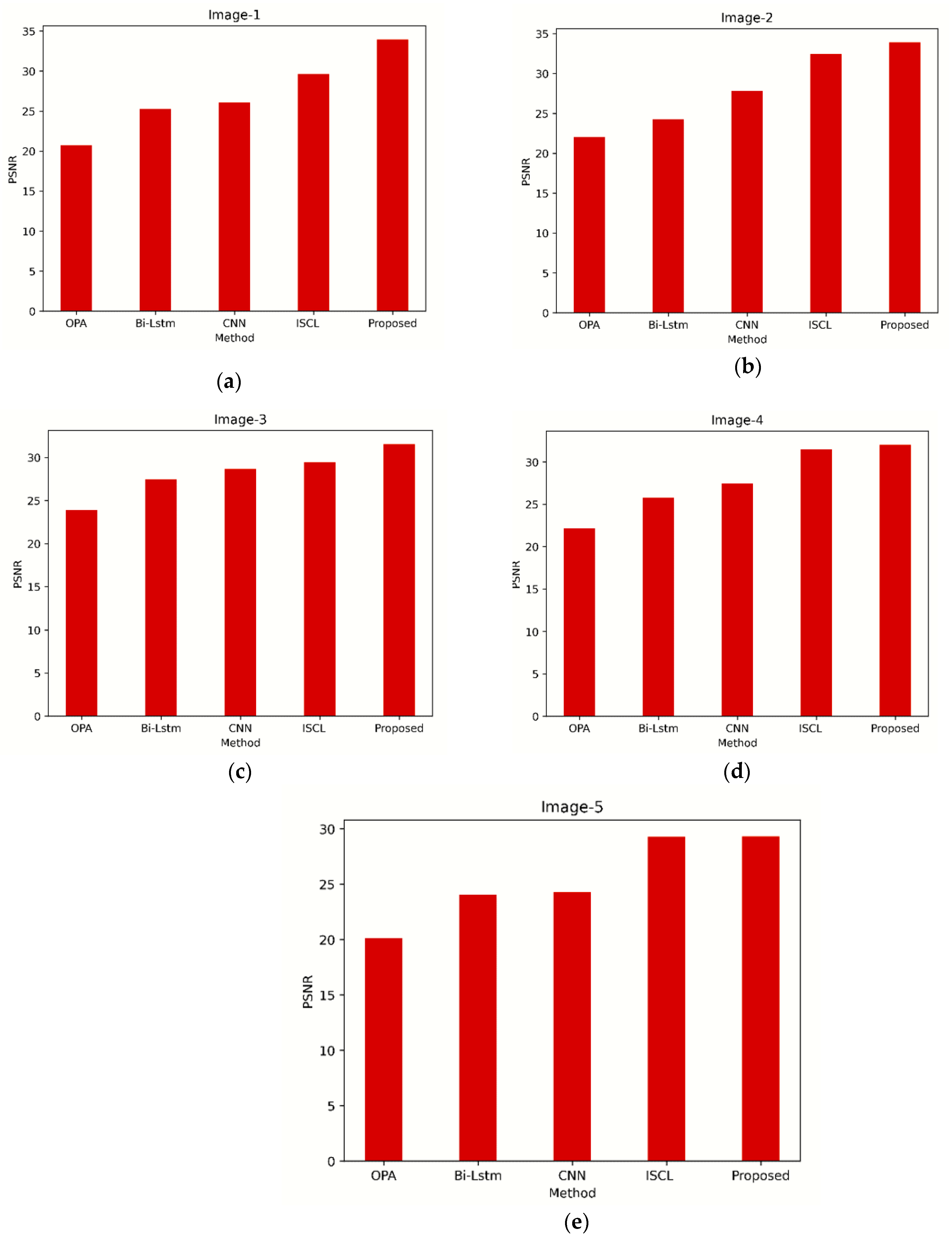
Table 2 presents the performance analysis of different existing algorithms proposed for PSNR. The suggested method yields an OPA of 25.309635 and a PSNR of 20.746605 for Image 1. Comparatively speaking to Bi-LSTM, CNN, and ISCL, the PSNR value is low [5]. In comparison to the other algorithms, the OPA value is moderate. The suggested method for Image 2 displays a PSNR of 22.015400, which is greater than Bi-LSTM but lower than CNN and ISCL [5]. The proposed method’s OPA (24.291343) is comparable to that of the previous algorithms. With a PSNR of 23.906961 for Image 3, the suggested method outperforms Bi-LSTM and ISCL [5] but falls just short of CNN. The proposed method’s OPA (27.426644) is competitive with those of the other algorithms. In contrast to Bi-LSTM and ISCL [5], the suggested technique for image four yields a high PSNR of 22.167478, indicating enhanced image quality. The proposed method’s OPA (25.754681) is competitive with those of the other algorithms. With a PSNR of 20.177721 for Image 5, the suggested method consistently outperforms other methods like Bi-LSTM and ISCL [5] but falls short of CNN. The proposed method’s OPA (24.068178) is competitive with those of the other algorithms.
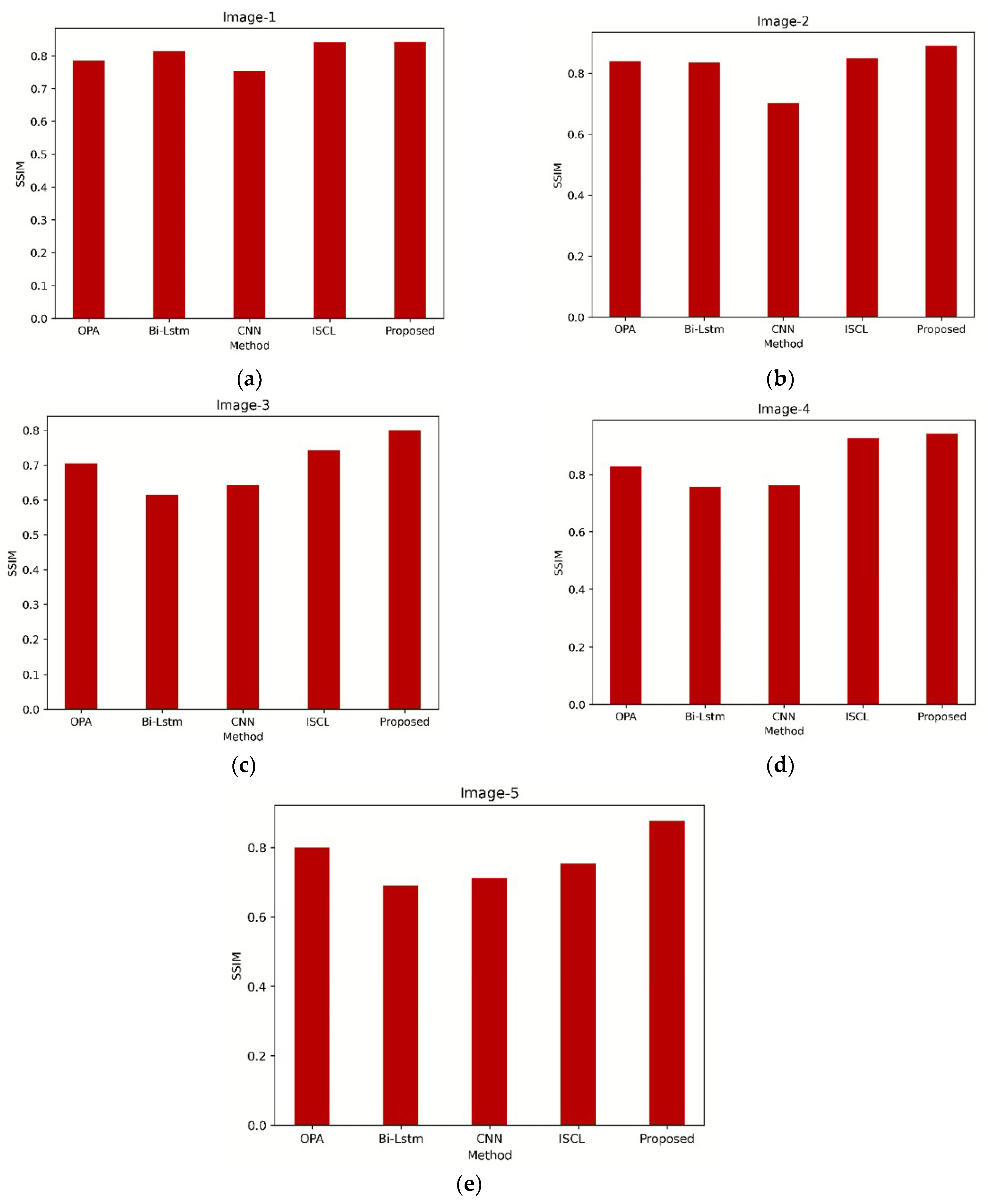
Table 3 presents the performance analysis of different existing algorithms proposed for SSIM. For Image 1, the proposed approach achieves an SSIM of 0.785890 and an OPA of 0.813365, which is comparable to the ISCL algorithm and higher than the Bi-LSTM and CNN algorithms. For Image 2, the proposed approach shows the highest SSIM of 0.890331, indicating better structural similarity compared to other algorithms. The OPA of the proposed approach (0.834619) is also competitive with the other algorithms. In Image 3, the proposed approach performs well with an SSIM of 0.799917 and an OPA of 0.704974, outperforming the Bi-LSTM, CNN, and ISCL algorithms. Image 4 demonstrates that the proposed approach achieves a high SSIM of 0.942487, indicating excellent structural similarity compared to other algorithms. The OPA of the proposed approach (0.755377) is also competitive with the other algorithms. In Image 5, the proposed approach performs consistently with an SSIM of 0.877609 and an OPA of 0.799414, surpassing the Bi-LSTM, CNN, and ISCL algorithms.

4.3. Overall Graphical Representation

The PSNR for the OPA, Bi-LSTM, CNN, ISCL, and the proposed model with hybrid Bi-LSTM with OPA is depicted in Figure 4. The quality of the reconstructed images is quantified by the PSNR metric, which measures the ratio between the power of the noise and the maximum possible power of the signal. The PSNR in the proposed method is better than existing works.
The SSIM values for the existing techniques and the proposed model are shown in Figure 5. The similarity between the original and reconstructed images is evaluated using the SSIM metric, which takes into account factors such as luminance, contrast, and structural content.
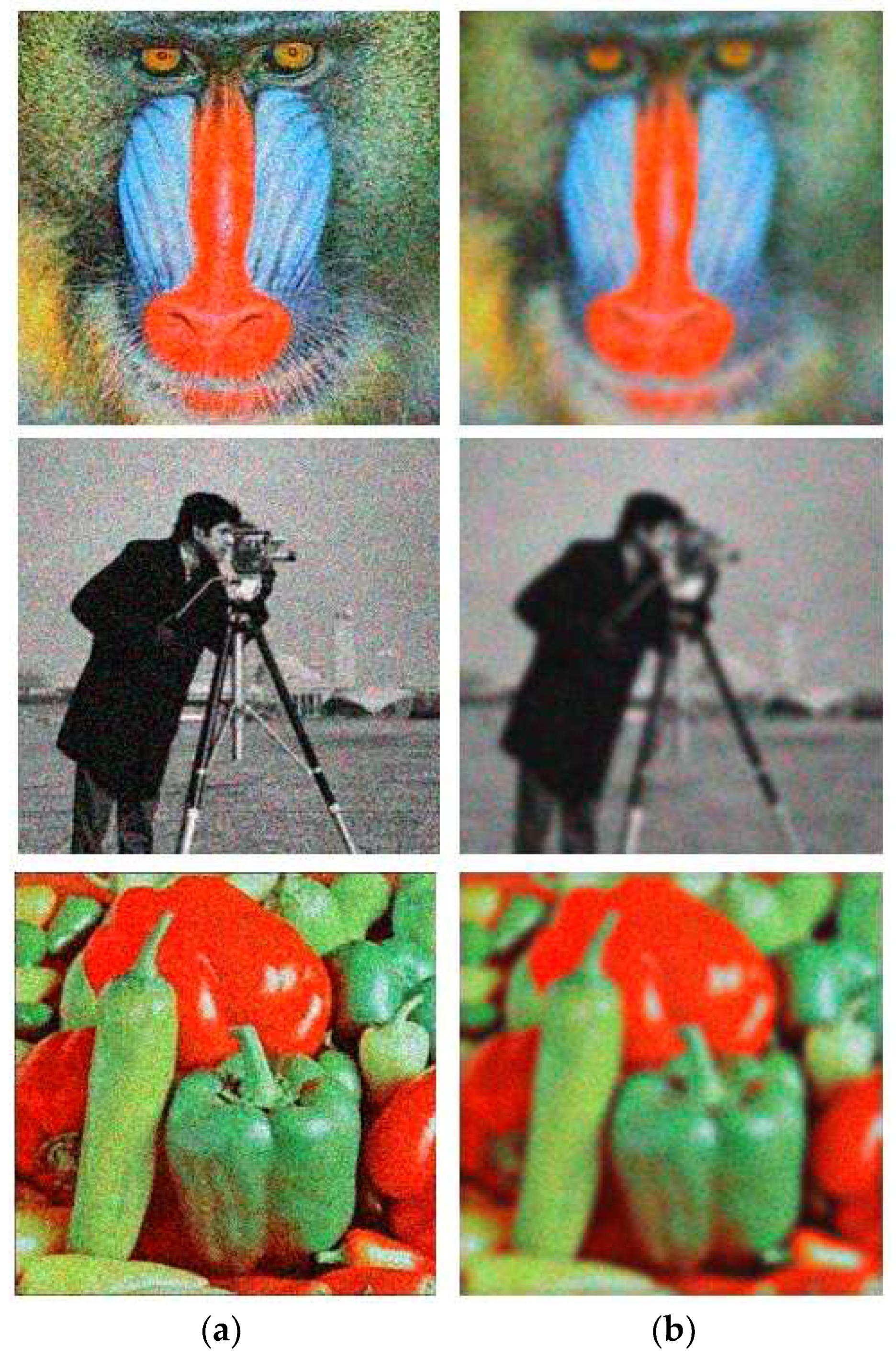
The denoising performance of the proposed model is demonstrated in Figure 6. The figure is divided into two subfigures: (a) showcases the original noisy images, and (b) presents the corresponding denoised images generated by the proposed model. Table 4 depicts the base paper comparison. Also, Table 5 and Table 6 show the statistical analysis and ablation study, respectively.

5. Conclusions

In computer vision, removing undesired noise from images is a critical task known as “image denoising”. Noise can drastically reduce the quality of an image, reducing its details, textures, and overall aesthetic appeal. It can come from a variety of sources, including sensor limits, transmission problems, and compression artifacts. Using the self-improved Orca Predation Algorithm (SI-OPA) for image denoising, this work proposed a revolutionary method that harnessed the power of hybrid deep learning. The suggested hybrid approach sought to improve denoising performance by combining the benefits of optimized Convolutional Neural Networks (CNN) and Bidirectional Long Short-Term Memory (Bi-LSTM). In particular, SI-OPA was used to specifically optimize the CNN’s weights, which enhanced performance and provided more precise noise removal. A detailed comparison with cutting-edge image denoising techniques was made to gauge the effectiveness of the suggested strategy. With a focus on denoising efficacy, computational economy, and preservation of image details and textures, the comparison covered a variety of conventional algorithms and deep learning-based solutions. The benefits and improvements provided by the suggested approach were emphasized through this comparative analysis, highlighting its potential as a promising option for image-denoising tasks. Python was used to put the proposed model into practice.

Author Contributions

Conceptualization, R.S.J., M.H.B.M.Z., D.A.H. and A.A.-N.; methodology, R.S.J., M.H.B.M.Z. and L.K.C.; formal analysis R.S.J., M.H.B.M.Z., D.A.H. and L.K.C.; investigation, R.S.J. and D.A.H.; resources, R.S.J.; data curation, R.S.J.; writing—original draft preparation, R.S.J. and D.A.H.; writing—review and editing, M.H.B.M.Z., A.A.-N. and L.K.C.; visualization, R.S.J., M.H.B.M.Z., L.K.C., D.A.H. and A.A.-N.; supervision, M.H.B.M.Z., L.K.C. and D.A.H.; project administration, M.H.B.M.Z., L.K.C., D.A.H. and A.A.-N.; funding acquisition, A.A.-N. and D.A.H. All authors have read and agreed to the published version of the manuscript.

Funding

This research received no external funding.

Data Availability Statement

Not applicable.

Conflicts of Interest

The authors declare no conflict of interest.

References

  1. Bayhaqi, Y.A.; Hamidi, A.; Canbaz, F.; Navarini, A.A.; Cattin, P.C.; Zam, A. Deep-Learning-Based Fast Optical Coherence Tomography (OCT) Image Denoising for Smart Laser Osteotomy. IEEE Trans. Med. Imaging 2022, 41, 2615–2628. [Google Scholar] [CrossRef]
  2. Liu, H.; Yousefi, H.; Mirian, N.; Lin, M.; Menard, D.; Gregory, M.; Aboian, M.; Boustani, A.; Chen, M.K.; Saperstein, L.; et al. PET Image Denoising Using a Deep-Learning Method for Extremely Obese Patients. IEEE Trans. Radiat. Plasma Med. Sci. 2022, 6, 766–770. [Google Scholar] [CrossRef]
  3. Wu, Q.; Tang, H.; Liu, H.; Chen, Y. Masked Joint Bilateral Filtering via Deep Image Prior for Digital X-Ray Image Denoising. IEEE J. Biomed. Health Inform. 2022, 26, 4008–4019. [Google Scholar] [CrossRef] [PubMed]
  4. Yang, Q.; Yan, P.; Zhang, Y.; Yu, H.; Shi, Y.; Mou, X.; Kalra, M.K.; Zhang, Y.; Sun, L.; Wang, G. Low-Dose CT Image Denoising Using a Generative Adversarial Network with Wasserstein Distance and Perceptual Loss. IEEE Trans. Med. Imaging 2018, 37, 1348–1357. [Google Scholar] [CrossRef]
  5. Lee, K.; Jeong, W.-K. ISCL: Interdependent Self-Cooperative Learning for Unpaired Image Denoising. IEEE Trans. Med. Imaging 2021, 40, 3238–3248. [Google Scholar] [CrossRef]
  6. Geng, M.; Meng, X.; Yu, J.; Zhu, L.; Jin, L.; Jiang, Z.; Qiu, B.; Li, H.; Kong, H.; Yuan, J.; et al. Content-Noise Complementary Learning for Medical Image Denoising. IEEE Trans. Med. Imaging 2022, 41, 407–419. [Google Scholar] [CrossRef] [PubMed]
  7. Li, Y.; Zhang, K.; Shi, W.; Miao, Y.; Jiang, Z. A novel medical image denoising method based on conditional generative adversarial network. Comput. Math. Methods Med. 2021, 2021, 9974017. [Google Scholar] [CrossRef] [PubMed]
  8. Sun, H.; Peng, L.; Zhang, H.; He, Y.; Cao, S.; Lu, L. Dynamic PET Image Denoising Using Deep Image Prior Combined with Regularization by Denoising. IEEE Access 2021, 9, 52378–52392. [Google Scholar] [CrossRef]
  9. Diwakar, M.; Singh, P. CT image denoising using multivariate model and its method noise thresholding in non-subsampled shearlet domain. Biomed. Signal Process. Control 2020, 57, 101754. [Google Scholar] [CrossRef]
  10. Tian, C.; Xu, Y.; Li, Z.; Zuo, W.; Fei, L.; Liu, H. Attention-guided CNN for image denoising. Neural Netw. 2020, 124, 117–129. [Google Scholar] [CrossRef] [PubMed]
  11. Dehner, C.; Olefir, I.; Chowdhury, K.B.; Jüstel, D.; Ntziachristos, V. Deep-Learning-Based Electrical Noise Removal Enables High Spectral Optoacoustic Contrast in Deep Tissue. IEEE Trans. Med. Imaging 2022, 41, 3182–3193. [Google Scholar] [CrossRef]
  12. Liu, N.; Wang, J.; Gao, J.; Chang, S.; Lou, Y. Similarity-informed self-learning and its application on seismic image denoising. IEEE Trans. Geosci. Remote Sens. 2022, 60, 5921113. [Google Scholar] [CrossRef]
  13. Prakash, M.; Krull, A.; Jug, F. Fully unsupervised diversity denoising with convolutional variational autoencoders. arXiv 2020, arXiv:2006.06072. [Google Scholar]
  14. El Helou, M.; Süsstrunk, S. Blind universal Bayesian image denoising with Gaussian noise level learning. IEEE Trans. Image Process. 2020, 29, 4885–4897. [Google Scholar] [CrossRef] [PubMed] [Green Version]
  15. Quan, Y.; Chen, Y.; Shao, Y.; Teng, H.; Xu, Y.; Ji, H. Image denoising using complex-valued deep CNN. Pattern Recognit. 2021, 111, 107639. [Google Scholar] [CrossRef]
  16. Tian, C.; Zheng, M.; Zuo, W.; Zhang, B.; Zhang, Y.; Zhang, D. Multi-stage image denoising with the wavelet transform. Pattern Recognit. 2023, 134, 109050. [Google Scholar] [CrossRef]
  17. Thanh, D.N.H.; Engínoğlu, S. An iterative mean filter for image denoising. IEEE Access 2019, 7, 167847–167859. [Google Scholar]
  18. Tian, C.; Xu, Y.; Zuo, W. Image denoising using deep CNN with batch renormalization. Neural Netw. 2020, 121, 461–473. [Google Scholar] [CrossRef]
  19. Geng, M.; Meng, X.; Zhu, L.; Jiang, Z.; Gao, M.; Huang, Z.; Qiu, B.; Hu, Y.; Zhang, Y.; Ren, Q.; et al. Triplet Cross-Fusion Learning for Unpaired Image Denoising in Optical Coherence Tomography. IEEE Trans. Med. Imaging 2022, 41, 3357–3372. [Google Scholar] [CrossRef] [PubMed]
  20. Tirer, T.; Giryes, R. Super-Resolution via Image-Adapted Denoising CNNs: Incorporating External and Internal Learning. IEEE Signal Process. Lett. 2019, 26, 1080–1084. [Google Scholar] [CrossRef] [Green Version]
  21. Dong, W.; Wang, H.; Wu, F.; Shi, G.; Li, X. Deep Spatial–Spectral Representation Learning for Hyperspectral Image Denoising. IEEE Trans. Comput. Imaging 2019, 5, 635–648. [Google Scholar] [CrossRef]
  22. Hashimoto, F.; Ohba, H.; Ote, K.; Teramoto, A.; Tsukada, H. Dynamic PET Image Denoising Using Deep Convolutional Neural Networks without Prior Training Datasets. IEEE Access 2019, 7, 96594–96603. [Google Scholar] [CrossRef]
  23. Kokkinos, F.; Lefkimmiatis, S. Iterative Joint Image Demosaicking and Denoising Using a Residual Denoising Network. IEEE Trans. Image Process. 2019, 28, 4177–4188. [Google Scholar] [CrossRef] [Green Version]
  24. Liu, D.; Wen, B.; Jiao, J.; Liu, X.; Wang, Z.; Huang, T.S. Connecting Image Denoising and High-Level Vision Tasks via Deep Learning. IEEE Trans. Image Process. 2020, 29, 3695–3706. [Google Scholar] [CrossRef] [Green Version]
  25. Wu, D.; Ren, H.; Li, Q. Self-Supervised Dynamic CT Perfusion Image Denoising with Deep Neural Networks. IEEE Trans. Radiat. Plasma Med. Sci. 2021, 5, 350–361. [Google Scholar] [CrossRef]
  26. Li, K.; Zhou, W.; Li, H.; Anastasio, M.A. Assessing the Impact of Deep Neural Network-Based Image Denoising on Binary Signal Detection Tasks. IEEE Trans. Med. Imaging 2021, 40, 2295–2305. [Google Scholar] [CrossRef] [PubMed]
  27. Ma, J.; Peng, C.; Tian, X.; Jiang, J. DBDnet: A Deep Boosting Strategy for Image Denoising. IEEE Trans. Multimed. 2022, 24, 3157–3168. [Google Scholar] [CrossRef]
  28. Chen, K.; Pu, X.; Ren, Y.; Qiu, H.; Lin, F.; Zhang, S. TEMDnet: A Novel Deep Denoising Network for Transient Electromagnetic Signal with Signal-to-Image Transformation. IEEE Trans. Geosci. Remote Sens. 2022, 60, 5900318. [Google Scholar] [CrossRef]
  29. Bahnemiri, S.G.; Ponomarenko, M.; Egiazarian, K. Learning-Based Noise Component Map Estimation for Image Denoising. IEEE Signal Process. Lett. 2022, 29, 1407–1411. [Google Scholar] [CrossRef]
  30. Wang, Z.; Ng, M.K.; Zhuang, L.; Gao, L.; Zhang, B. Non-local Self-Similarity-Based Hyperspectral Remote Sensing Image Denoising with 3-D Convolutional Neural Network. IEEE Trans. Geosci. Remote Sens. 2022, 60, 5531617. [Google Scholar]
  31. Le, T.; Vo, M.T.; Vo, B.; Hwang, E.; Rho, S.; Baik, S.W. Improving electric energy consumption prediction using CNN and Bi-LSTM. Appl. Sci. 2019, 9, 4237. [Google Scholar] [CrossRef] [Green Version]
  32. Albawi, S.; Bayat, O.; Al-Azawi, S.; Ucan, O.N. Social touch gesture recognition using convolutional neural network. Comput. Intell. Neurosci. 2018, 2018, 973103. [Google Scholar] [CrossRef] [PubMed] [Green Version]
  33. Emam, M.M.; El-Sattar, H.A.; Houssein, E.H.; Kamel, S. Modified orca predation algorithm: Developments and perspectives on global optimization and hybrid energy systems. Neural Comput. Appl. 2023, 35, 15051–15073. [Google Scholar] [CrossRef]
  34. Myntra Fashion Product Dataset. Available online: https://www.kaggle.com/datasets/hiteshsuthar101/myntra-fashion-product-dataset (accessed on 25 May 2023).
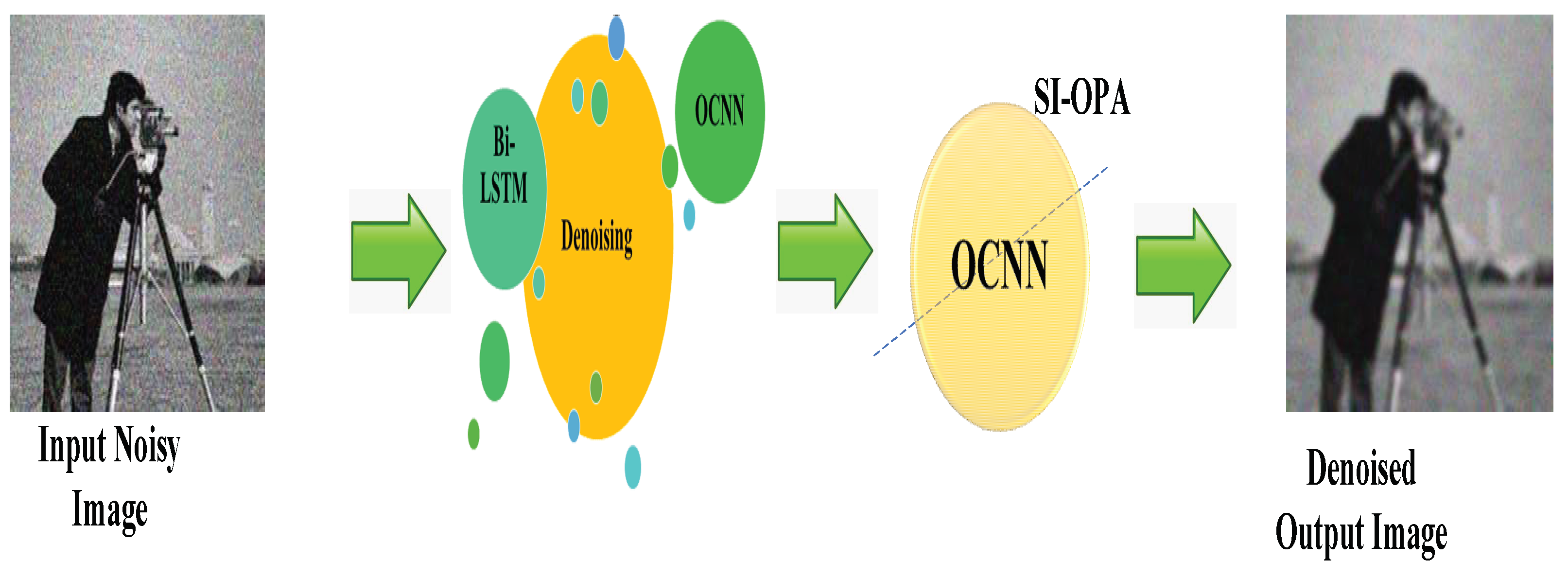
Figure 1. Overall proposed architecture.
Technologies 11 00111 g001
Figure 2. Bi-LSTM.
Figure 2. Bi-LSTM.
Technologies 11 00111 g002
Figure 3. Optimized CNN.
Technologies 11 00111 g003
Figure 4. PSNR (a) Image 1 with OPA, Bi-LSTM, CNN, ISCL, and Hybrid Bi-LSMT with OPA, OPA, LSTM (b) Image 2 with OPA, Bi-LSTM, CNN, ISCL, and Hybrid Bi-LSMT with OPA (c) Image 3 with OPA, Bi-LSTM, CNN, ISCL, and Hybrid Bi-LSMT with OPA (d) Image 4 with OPA, Bi-LSTM, CNN, ISCL, and Hybrid Bi-LSMT with OPA and (e) Image 5 with OPA, Bi-LSTM, CNN, ISCL, and Hybrid Bi-LSMT with OPA.
Technologies 11 00111 g004
Figure 5. SSIM (a) Image 1 with OPA, Bi-LSTM, CNN, ISCL, and Hybrid Bi-LSMT with OPA, OPA, LSTM (b) Image 2 with OPA, Bi-LSTM, CNN, ISCL, and Hybrid Bi-LSMT with OPA (c) Image 3 with OPA, Bi-LSTM, CNN, ISCL, and Hybrid Bi-LSMT with OPA (d) Image 4 with OPA, Bi-LSTM, CNN, ISCL, and Hybrid Bi-LSMT with OPA and (e) Image 5 with OPA, Bi-LSTM, CNN, ISCL, and Hybrid Bi-LSMT with OPA.
Technologies 11 00111 g005
Figure 6. (a) Original noise images (b) Denoised images.
Technologies 11 00111 g006
Table 1. Research Gaps.
AuthorAimMethodsAdvantageDisadvantage
Wu et al. [25]Develop self-supervised deep learning for CTP denoising without high-dose reference images, improving acute ischemic stroke diagnosis.Train network to map CTP frames, removing noise independently in the source and target, validated on real and simulated datasets.Eliminates need for high-dose images, facilitates adaptation to different protocols and improves image quality, spatial resolution, and contrast-to-noise ratio.Performance reliant on dataset quality and size, potentially limited effectiveness if dataset is limited or biased.
Ma et al. [27]Introduce DBDnet, a deep boosting denoising net, to improve image denoising by eliminating noise of the noise map.Utilize residual learning to generate a noise map and progressively reduce noise of the noise map via boosting function.Effective denoising, theoretical analysis, NoN-eliminating module outperforms state-of-the-art methods in Gaussian and real image denoising.Performance subject to noise levels, potential sensitivity to input variations and computational complexity not discussed in detail.
Bahnemiri et al. [29]Propose a deep CNN-based method for estimating sigma-map to address non-stationary noise in image denoising.Use deep CNN to estimate a local patch-wise standard deviation map (sigma-map) for non-stationary noise removal.Achieves state-of-the-art accuracy in sigma-map estimation for non-stationary noise and outperforms other methods in denoising flexibility and PSNR.Still requires noise estimation, performance may vary based on noise levels, CNN-based approach may have computational overhead.
Li et al. [26]Evaluate DNN-based denoising methods for medical images using task-based IQ measures to assess their impact on signal detection tasks.Employ task-based IQ measures for binary signal detection tasks under SKE with BKS conditions to quantify denoising impact.Provides objective evaluation of DNN-based denoising methods and assesses denoising network depth’s impact on task performance.Task-specific evaluation may not cover all aspects of denoising, limited to binary signal detection tasks in specific conditions.
Hashimoto et al. [22]Propose dynamic PET image denoising using a deep image prior (DIP) approach without pre-training or large datasets.Employ DIP method with static PET data as input and dynamic PET images as labels for denoising.Doesn’t require large datasets or pre-training, produces less noisy and more accurate dynamic PET images and is applicable to low-dose PET imaging.Limited to PET image denoising, may not fully generalize to other medical imaging tasks or modalities.
Table 2. Existing and proposed performance analysis.
PSNROPABi-LSTMCNNISCLProposed
Image 120.74660525.30963526.05735729.67080133.970612
Image 222.01540024.29134327.80325029.93592132.459123
Image 323.90696127.42664428.67796729.45338331.565056
Image 422.16747825.75468127.45289030.04543231.476256
Image 520.17772124.06817824.27898629.26461329.340515
Table 3. Existing and proposed performance analysis.
SSIMOPABi-LSTMCNNISCL Proposed
Image 10.7858900.8133650.7538390.8401160.841548
Image 20.8401240.8346190.7022830.8495320.890331
Image 30.7049740.6146220.6443790.7429190.799917
Image 40.8273430.7553770.7625490.9270480.942487
Image 50.7994140.6898100.7114970.7534330.877609
Table 4. Base paper comparison.
MetricsCGAN—JSRT Datasets [7]SURE-LET [9], σ = 20Proposed
PSNR33.26423.567733.9706
SSIM0.92060.82340.8415
Table 5. Statistical analysis.
Statistical AnalysisOPABi-LSTMCNNISCL [5]Proposed
Image 10.7915490.7415590.7149100.8226100.870378
Image 20.7994140.7553770.7114970.8401160.877609
Image 30.0529850.0905510.0472510.0759520.053493
Image 40.7049740.6146220.6443790.7429190.799917
Image 50.8401240.8346190.7625490.9270480.942487
Table 6. Ablation Study.
AblationD = 3D = 5D = 10D = 15D = 20
Image 10.8295470.8241120.6934410.8388360.879122
Image 20.6960990.6068840.6362660.7335660.789846
Image 30.7759950.8031250.7443480.8295390.830953
Image 40.7893490.6811250.7025400.7439470.866560
Image 50.8169270.7458670.7529490.9153770.930621
Disclaimer/Publisher’s Note: The statements, opinions and data contained in all publications are solely those of the individual author(s) and contributor(s) and not of MDPI and/or the editor(s). MDPI and/or the editor(s) disclaim responsibility for any injury to people or property resulting from any ideas, methods, instructions or products referred to in the content.