Abstract
This paper focuses on the relationship between the European Union Emission Trading System allowances’ prices and the Italian electricity price, aiming at assessing whether such a mechanism has been a driver for the decarbonization of the power sector. To this aim, we calculate the long-run relationships between energy prices, natural gas prices and allowances’ prices, through a VECM model, distinguishing between peak and off-peak prices. The analysis is carried out for the third phase of the EU-ETS, which started in 2013, and for two-year rolling windows that account for changes over time of the pass-through rates. It is shown that the natural gas price has a high pass-through rate of roughly 70%, which is increasing over time. On the contrary, the pass-through rate of the allowances’ price is as low as 7% for the wholesale electricity price, being slightly more and less for the peak and off-peak prices, respectively. However, this rate has been substantially changing over time, starting from a high level and falling significantly, becoming negative in the recent years. This could signal that the EU-ETS has been increasingly more effective in endogenizing emission costs for power producers, inducing them to reduce their production costs associated with emissions by means of a change in technologies. However, the analysis of the impulse response functions hardly supports this finding, eventually casting doubts on the effectiveness of the EU-ETS in Italy to drive the transition toward a less carbon-intensive power supply.
1. Introduction
The Emissions Trading System of the European Union (EU-ETS) is a cap-and-trade system, introduced to fight climate change and to accomplish the reduction targets of the Kyoto protocol. It sets a cap to the total amount of greenhouse gases (GHGs) that can be produced by the installations covered by the system, which is set to decrease over time to reduce the total amount of emissions. A market of allowances (EUA), representing a permit to emit a ton of CO2, is established. Power producers can use the allowances they own either to sell them to other market participants or to cover the greenhouse gas emissions resulting from their power production. Allowances are, therefore, financial products, exchanged in financial markets (Cludius and Betz 2020; Daskalakis et al. 2009; Graham et al. 2016; Harasheh and Amaduzzi 2019). By using the allowances to produce electricity, one bares the opportunity cost of losing their financial value. Rationally, power producers should respond to an increase in costs due to a rise in the value of the allowances by adopting low-emitting technologies. This happens if the rise in costs is perceived as permanent and if prices cannot be raised to shift the burden of the allowances to the final consumers. As a consequence, whenever power producers perceive the cost of the allowances as a relevant component of their production costs and they are not able to rise their bids in the wholesale market, they should progressively respond to an increase in the allowance price by reducing the power production costs. They can do so by minimizing the extent to which they use less efficient (i.e., more emitting) power plants, or by adapting their production portfolio mix to increase the share of plants fueled by renewable energy sources (from now onward, RES-plants). These solutions should increase the share of RES energy in the energy system, lower the amount of emissions, and induce a decreasing wholesale (electricity) price. This is perfectly in line with the “polluters pay” principle when applied to greenhouse gas emission in the power production sector. However, the ability of the EU-ETS to effectively endogenize emissions’ cost relies on the impossibility to shift the burden of the policy to final consumers. The extent to which the CO2 emission costs can be passed to the buyers through an increase in the electricity price is defined as the pass-through rate. It is therefore crucial to evaluate whether and to what extent emission costs of the EU-ETS can be shifted to final consumers. Many empirical studies have tackled such a research question. Most of these studies focus on the first two phases of the EU Emission Trading System (from 2005 to 2007, and from 2008 to 2012, respectively), finding a relevant and high pass-through rate of EUA costs into electricity prices, yet with a large range. Sijm et al. (2006) report a cost pass-through of about 60–117% for Germany, and of 64–81% for the Netherlands. Sijm et al. (2008) extend this analysis and find a positive but incomplete carbon cost pass-through in the Netherlands, Germany, France and Sweden, and a full pass-through in the U.K. market. Fabra and Reguant (2014) measure a pass-through rate for Spain that differs between peak and off-peak hours, and ranges from 70% to 140% for the former and from 28% to 97% for the latter, depending on the model used. Honkatukia et al. (2008) find a pass-through that ranges between 75% and 95% when analyzing the Finish Nord Pool electricity spot prices. Hintermann (2016) establishes a pass-through that ranges between 81% and 111% for the wholesale electricity price in Germany. Jouvet and Solier (2013) consider a set of European countries and, by analyzing both the first and (a part of) the second period of the EU-ETS, they show that the pass-through rates are less relevant during the second phase and even negative in some countries. Other scholars have also found limited pass-through rates. Bariss et al. (2016) find a 55% pass-through rate in the Nordic market and a 65% pass-through rate in Baltic countries. Bunn and Fezzi (2008) show that the pass-through rates can be as low as 42%. For Ahamada and Kirat (2015), the pass-through rates of the French and German electricity baseload prices during the second phase of the EU-ETS are even lower, roughly around 18%. Ahamada and Kirat (2018) further show that the pass-through rate is non-linear and dependent on the threshold levels of the allowances’ prices. Similarly, using futures on electricity, very low pass-through rates are obtained for Germany, France, Belgium and the Netherlands by Lo Prete and Norman (2013). Chernyavs’ka and Gulli (2008) follow a different approach and instead of relying on econometric analysis, they simulate the load duration curve and the merit order supply curve for two zones of the Italian market, showing that the pass-through depends on whether it refers to peak or off-peak hours and on the level of competition across producers.
In our paper, we aim at assessing the effectiveness of the EU-ETS in endogenizing emission costs and, therefore, in driving energy transition toward a less carbon-intensive power mix in Italy. To do so, by considering the most recent changes occurred in the third phase of the regulation, we test whether there is a relevant pass-through of the allowances price in the Italian electricity price, and whether there is a significant impact of EU-ETS costs in the final power price. A high pass-through rate would signal the relative ability of power producers to adapt to the EU-ETS regulation without the need for reducing their emissions in the attempt to decrease the allowances’ costs, and vice versa. By identifying the presence of cointegration between the allowances’ prices, gas prices and Italian electricity prices, we are able to analyze the long-run relationship between these variables. To see how such a relationship has changed over time, a dynamic analysis is set up, performing the cointegration analysis on two-year rolling windows for the whole period of observation (from the beginning of the third phase of the EU-ETS until the end of 2018). This provides a measure of how the pass-through of the EU-ETS costs has changed over time.
The European Emission Trading System is characterized by a total emission cap which is set to decrease over time: this translates into increasing costs for producers. For this reason, it is important to study the evolution of the regulatory framework in its most recent phase, using a dynamic approach, which is the major contribution of this study. Note, however, that the presence of cointegration is only a sufficient, not necessary, condition for a pass-through to happen. The correlation among electricity and allowances’ prices in the long run can, in fact, be determined by other factors, such as an increasing share of RES in the power production mix. If that were the case, the EU-ETS would be finally successful in reaching its reduction goals through a change in technologies caused by the “polluters pay” principle. To test for such a hypothesis, we finally study the impulse response functions, showing which variables adjust to bring the system back to the long-run equilibrium.
The paper is structured as follows. In Section 2, the methodology is introduced. Section 3 displays the results. Section 4 discusses the policy implications. References follow. Appendix A contains data summary statistics and graphical analyses, stationarity tests and impulse response functions for Models 2 and 3.
2. Materials and Methods
The Italian PUN (Prezzo Unico Nazionale), which is traded in the MGP, the Italian day-ahead market, is used as a proxy for the wholesale power price in Italy. Indeed, Italy is a zonal market in which the power selling price differs across zones while purchase offers are valued at the single weighted average of zonal prices. The electricity data are retrieved directly from the GME’s webpage, while the allowances’ prices are obtained from the European Climate Exchange (EEX), the most liquid platform for this type of product. In detail, we adopt the prices of the EEX futures contracts, which are expressed in euros per ton. Each contract represents 1000 emission allowances. In addition to the EUAs prices, our dataset includes Italian PSV (punto di scambio virtuale—virtual trading point) natural gas future prices. Appendix A.1 provides summary statistics of all the variables and their graphical representation. All data were collected from January 2013 to December 2018.
Electricity hourly prices are transformed into daily prices, with the exclusion of weekends, through a weighted average, where the total volumes exchanged are used as weights. This allows us to compare the electricity prices with the daily CO2 prices, which we collected from the Refinitiv Eikon database. Moreover, by averaging daily prices, we control for intraday volatility and intraday price patterns: in this way, we can focus on the determinants of prices, which include emission costs. In addition, by excluding the weekends, we remove the most relevant component of the periodic evolution of electricity prices. Consequently, there is no need to introduce further seasonal adjustments on the electricity prices. Finally, as far as the analyses are concerned, we first consider the whole set of hourly prices, and we later distinguish between peak and off-peak prices. The latter distinction allows to take into consideration the differences in the marginal technology that occur between peak and off-peak hours.
In the preliminary analyses (see Appendix A.2), we use the bound testing methodology, suggested by Pesaran et al. (2001), to identify the presence of cointegration in cases where statistical tests do not univocally indicate the stationarity properties of the series of interest. Having identified the existence of cointegration, we follow the Johansen approach (Johansen 1991, 1988, 1995) and set the following vector error correction model (VECM):
where is the vector including the log-prices of energy,1 gas and allowances, denotes first-order differencing, while , , , … are parameter matrices, and is an innovation term which is assumed to be with a zero mean and with a covariance matrix equal to . Notably, the VECM framework is flexible enough to allow for the presence of deterministic terms in both the cointegrating relations as well as in the dynamic evolution of the differenced variables. The trace and maximum eigenvalue tests of Johansen (1995) are used to identify the number of cointegration relations. The tests’ critical values depend on the presence of deterministic relations and on the lag order p. In our case, we specify the model with an intercept in both the cointegration relation and in the VECM, and we use 5 lags. The model estimation follows the Johansen approach (Johansen 1995). We consider two possible cases: in the first one, we include in the model three variables (the overall wholesale electricity (PUN) price, the allowances price and the gas price); in the second case, we substitute the PUN price by its peak and off-peak components, respectively (PUNp and PUNop). Results are presented in Table 1 and Table 2 (* = statistically significant at 10% level).

Table 1.
The Johansen test of cointegration. Electricity price: PUN.
Table 2.
The Johansen test of cointegration. Electricity prices: peak and off-peak PUN.
In both cases, the tests are concordant and identify the presence of cointegration. While in the first case, a unique cointegrating relation is detected, in the second model, two relations are identified. This evidence is in line with the expectations. On the one hand, the role of allowances and gas in determining the energy price is associated with their role in the production process since they are both production costs. This justifies the long-run relationship with the electricity price. On the other hand, when peak and off-peak prices are separated, different levels of loads and prices are included in the model and, as a consequence, both prices can be related by a cointegration relation to gas and allowances.
Given the existence of cointegration, restrictions can be imposed on the structure of matrix . Indeed, under cointegration, matrix has a reduced rank, and its rank corresponds to the number of cointegrating relations that exist among the modeled variables. Matrix can be, therefore, decomposed into the product of two matrices, , including the cointegration vectors that contains the parameters linking the log-prices in equilibrium (or, equivalently, in the long-run), and , the matrix of adjustment coefficients, capturing the speed of convergence toward the equilibrium of the variables in the model. The model specification we expect has thus the following structure, obtained by rearranging Equation (1):
where we set the lag order to 5, capturing up to a weekly lag. In this bivariate case, the term becomes
where we point out that the first element of the vector is normalized to 1. Differently, when we do have two cointegrating relations, we have
where the two long-run relations include just one price, which follows from traditional identification schemes adopted for VECM.
From the VECM model, one might also recover the impulse response functions (IRF), allowing to track the evolution of the target variable in response to a shock on a given variable. In our analyses, we recover the IRF from the VAR companion representation of the VECM, namely,
The IRF are evaluated after a unitary shock on the orthogonal residual such that . Note that the covariance matrix of the residuals is the identity matrix and the covariance matrix of satisfies .
3. Results
The estimates of the cointegrating equations are summarized in Table 3. Note that since the model is run in logarithms, betas can be interpreted as elasticities. Consequently, the beta relative to the allowances’ price is our variable of interest, i.e., the pass-through rate. The table reports the estimate of the three variable specifications defined in Equation (3) for three different cases: Model 1 uses the PUN, Model 2 the peak prices, and Model 3 the off-peak prices. The last case, Model 4, refers to the specification that includes both peak and off-peak prices, defined in Equation (4).
Table 3.
The cointegrating equation.
Overall, the results confirm that the models fit well. All the betas are significant, at least at the 10% level. The results in Column 1 show that an increase in the natural gas price and in the price of the allowances is correlated with an increase in the Italian electricity price. Natural gas has a huge impact on the electricity price: a EUR 1 increase in the gas price produces, in the long-run, a 72-cent increase in the PUN. On the other hand, the impact of the allowances is more limited: a EUR 1 increase in the EUA is reflected in a modest 7-cent increase in the Italian electricity price. Results are confirmed in columns 2 and 3, which report the coefficients for the peak and off-peak prices, respectively. It can be noticed that the pass-through rates are almost equivalent, with a more moderate impact of the allowances during off-peak hours and a higher one for the peak prices. Similar figures are obtained for Model 4, the last two columns, which confirm that when we consider together the cointegrating relationships between natural gas and allowances prices with peak and off-peak electricity prices, there is a significant yet modest pass-through rate of the allowances’ prices into both peak and off-peak ones.
The limited pass-through rates of the allowances are in line with what is shown by Jouvet and Solier (2013) for the Italian markets. They show that, when considering only data of the first two phases of the EU-ETS, in Italy, it is possible to “[…] reasonably conclude that carbon costs were not yet passed through on spot markets over the second phase of the EU ETS.” (Jouvet and Solier 2013, p. 1375). Note that a positive (although small) pass-through rate is not efficient since it allows polluters to partially shift the burden of their emissions to end consumers.
The significance of the electricity price in the α vector reported in the second part of the table indicates that the direction of the long-run adjustment goes from gas prices and allowances costs toward the PUN. More precisely, it indicates that when the average electricity price is too high, it slowly falls back toward the equilibrium. This is the case for the three single-price models (1, 2 and 3). In the four-variate model (4), interestingly enough, the evidence shows that off-peak prices react to both peak and off-peak prices, while the opposite is not true. This might signal a strategic behavior of power producers during off-peak hours, where they can bid considering both off-peak and peak prices.
We then investigate the dynamic pass-through effect, calculating the pass-through for a window of two-years observations that is rolling every month throughout the sample period. For clarity of exposition, only Models 1, 2 and 3 are considered: the beta coefficients (and their confidence intervals) relative to both gas and allowances prices are plotted in Figure 1.
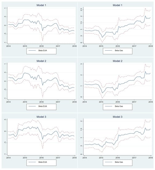
Figure 1.
Rolling analysis for Models 1, 2 and 3. The graphs show the beta coefficients (and their relative confidence intervals) for allowances (left-hand side) and natural gas (right-hand side) resulting from the rolling analysis.
It can be noted that the coefficients change significantly throughout the observation period. In particular, the pass-through rate of gas prices rises over time in all three model specifications. On the contrary, when considering the first model, the pass-through rates captured by the beta of the allowances (EUA) show an opposite trend (although less evident), going from a positive pass-through rate of almost 30% to a negative figure of roughly the same amount. This is even more striking when we look at the peak PUN (Model 2), for which the allowances pass-through rates go from a maximum of almost 50% to a minimum of 40% in the last rolling window. For the off-peak PUN, the dynamics have been equivalent, yet, with lower variations.
A drop in the pass-through rate suggests that, in the most recent years, the Italian electricity price tends to move less after a change in the allowances price. This could signal that the EU-ETS has been increasingly more effective in endogenizing emission costs for power producers, making them decrease the portion of production costs associated with their emissions. However, the mere (falling) correlation across these prices does not guarantee that a real interconnection among allowances and electricity prices exists also in the short run. To gain insight on the causality order and see whether, in the short run, a change in the allowances price (or natural gas one) impacts the electricity price or vice versa, or both, the impulse response functions of the models are evaluated. They are reported in Figure 2 and Figure 3. Figure 2 plots the impulse response functions of Model 1, i.e., the model that does not make any distinction between peak and off-peak prices, for up to 40 lags (8 weeks), and with a 90% confidence interval to evaluate their statistical significance (confidence intervals are obtained through bootstrap). Notably, the correlations among the VECM changes are very small, close to zero in most cases. The largest value is registered between allowances and gas changes, equal to 0.16. Consequently, unitary shocks on the orthogonalized residuals ηt are almost equivalent to shocks on the correlated residuals εt (see Equation (5)) and the IRFs are very close to those obtained after a one standard deviation shock on the VECM residuals. Given these strong similarities, the IRFs can be interpreted as if they were obtained with a one standard deviation shock on the correlated residuals (i.e., non-orthogonalized). In the tri-variate model, the standard deviations of the shocks are around 0.091 for the energy price, 0.017 for gas and 0.033 for allowances. Differently, in the four-variate model, 0.118 is for peak prices, 0.081 for off-peak prices, and for gas and allowances, they are comparable to the previous ones.
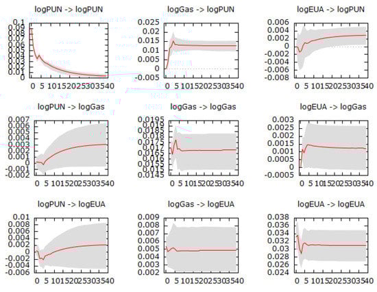
Figure 2.
Impulse response functions of the VECM Model 1 (three variables, PUN, and one cointegration relation). The shaded area represents the 90% confidence interval.
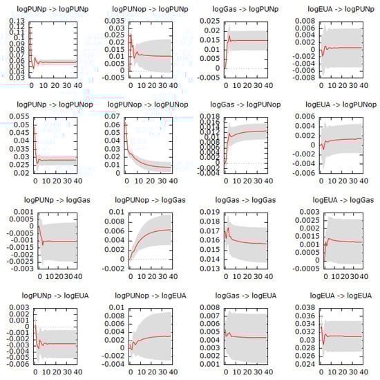
Figure 3.
Impulse response functions of the VECM Model 4 (four variables, peak and off-peak PUN, two cointegration relations). The shaded area represents the 90% confidence interval.
As expected, some of the IRFs converge to non-null values since non-stationary series are being considered. The diagonal elements of the IRF matrix are always statistically significant. It can be noted that shocks on the gas price transmit in large part to the energy price, with an IRF stabilizing with high significance around 0.0125 after a shock of 0.017. However, shocks on the allowances lead only to a marginally statistically significant impact on the energy prices after four weeks; the impact, in the long run, has a size comparable to that of the shock. Finally, across the remaining off-diagonal IRFs in Figure 2, only in one other case there are statistically significant reactions: allowances react to a gas price shock, with reactions much smaller than the shock size.
The IRF are evaluated also for Models 2 and 3, replacing the electricity price with either the peak or off-peak price, confirming the previous elements. Appendix A.3 includes those figures.
Figure 3, that takes into consideration a four-variate model, confirms the relevant impact of gas price shocks on the energy prices. A shock, in the long run, is fully transmitted. Allowances do not impact the prices’ evolution. On the contrary, there is a significant, yet limited, negative impact going from the peak prices to the allowances. This seems to signal that, effectively, peak prices influence allowances’ prices and not vice versa. A possible explanation might depend on the dynamics of power markets and allowances market. A rise in peak price can be due to a shortage in supply. Given that the capacity installed is fixed, this can signal power outages from some power plants, that would not be demanding allowances in the market, as they would not need to cover their missed production. This reduction in demand can have a negative impact on the allowances’ price.
4. Conclusions
The EU Emission System, firstly introduced in 2005, is now at its third phase after a continuous process of refinement and improvement. One of its key elements is the emission permits, i.e., allowances, whose price is bound to increase over time as a consequence of the decreasing cap on the total emissions. Allowances are a component of the variable costs of (thermal) power production. Power producers can react to the increase in the price of the allowances by (partially) passing them on the final electricity price or, on the contrary, by reducing their emissions through a technological change. Our study analyzes the relationship between the price of the allowances and the electricity price in the Italian market, which is one of the biggest European markets in terms of size and electricity price level, focusing on the last phase of this regulatory framework (third phase of the EU-ETS). The analysis of the relationship among these prices can detect the presence of pass-through, which, if positive, would hinder the ability of the scheme to provide the correct incentive toward the decarbonization of the power sector.
Thanks to a dynamic approach, it is possible to see if the EU-ETS is effective in endogenizing emissions’ costs for thermal power production or if producers have adapted to it by passing through the cost of the allowances to end consumers. We show that there is a limited pass-through of emissions costs in the third phase: a EUR 1 rise in the allowances’ price is coupled with a 7-cent rise in the electricity price. Moreover, the pass-through rate has been falling significantly over time.
The falling pass-through rate can indicate a technology substitution effect induced by the allowances’ cost. In particular, if the rising price of the allowances is perceived as a permanent component of the production cost by thermal power producers, they can respond over time by changing technology, replacing net CO2 emitting technologies with less emitting technologies, or even carbon-neutral ones. However, this depends also on the degree of competitiveness of power markets. The more that players have market power, the less the system marginal price would reflect the cost structure of power generation of the marginal plants. Therefore, the substitution effect can take place only if the market is sufficiently competitive. At first sight, this is what has happened in the structure of the power production in Italy during the third phase of the EU-ETS, which experienced a large penetration of RES-fueled generation capacity that has replaced the share of large CO2 emitters (in particular, oil and coal plants). In particular, the share of power produced by RES in Italy increased from 33.9% in 2013 to 40.83% in 2018, with the final goal for renewables to surpass natural gas as the primary fuel for electric power generation by 2020. In the power market, the increase in electricity produced by RES-fueled plants lowers electricity prices since these plants produce at null or low marginal costs. This is what happened in Italy, which experienced a decrease in the average day-ahead price, which can hardly be explained by market power since the Italian wholesale market is quite competitive, at least in its biggest zone, North (note, however, that a precise assessment of the degree of competitiveness and its impact on the day-ahead price goes beyond the scope of the present paper). However, the reduction in electricity price, captured by a negative pass-through rate and an increasing price of the allowances, is not necessarily caused by a variation in the emissions cost component. The negative pass-through rates do not imply per se that the causality order necessarily goes from the allowances prices to the electricity ones through the technical substitution effect. Indeed, the rise in RES-plants production and in allowances’ prices might be induced by some policy-driven technological changes (such as incentive policies, regulatory changes in the electricity sector, more stringent environmental rules and similar).
The study of the impulse response functions of the VECM can shed a light on this issue by detecting the causality orders (if there are any) running across the variables of interest. The analysis shows that changes in the long-run equilibrium of the electricity price (be it the overall PUN or disentangled in peak and off-peak prices) are not caused by the allowances’ prices. In other words, data cannot support the claim that the long-run relationship (which is shown to exist) between electricity and allowances’ prices is affected by short-run changes in such a way that, when the allowances’ price rises, the electricity price adjusts accordingly, returning to the long-run equilibrium.
This casts some doubts on the impact that the EU-ETS mechanism has had in endogenizing emissions costs, implementing the “polluters pay” principle and inducing an increase in RES-plants penetration in the case of Italian power production. In other words, it seems that the allowances have not been able to finance the energy transition of the Italian power system (note, however, that most of the Italian thermal capacity participates also in the balancing market; the thermal power capacity can derive a relevant share of its profit from that market; and the analysis of the relationship between the ETS and the balancing price might shed further light on the pass-through rate, but this goes beyond the scope of the present paper). This does not mean that the system is inefficient as a whole.2 The “trading” nature of the EU-ETS, in fact, makes the cut in emissions happen in those sectors where it is more efficient to do so, eventually reaching its primary goal of lowering the emission levels in Europe. As a consequence, regulators must put particular attention on those sectors where this does not happen, providing additional incentives when necessary, including proper tools to hedge climate-related sector-specific risks3.
Author Contributions
Conceptualization, F.F.; methodology, M.C. and F.F.; software, M.C. and S.S.; validation, M.C., F.F. and S.S.; formal analysis, M.C. and S.S.; investigation, M.C., F.F. and S.S.; resources, M.C., F.F. and S.S.; data curation, S.S.; writing—original draft preparation, M.C., F.F. and S.S.; writing—review and editing, M.C. and F.F.; visualization, M.C. and S.S.; supervision, M.C. and F.F. All authors have read and agreed to the published version of the manuscript.
Funding
This research received no external funding.
Data Availability Statement
The Italian PUN prices and the PSV can be found at https://www.mercatoelettrico.org/It, accessed on 8 October 2021; future prices on the EEX platform can be retrieved at https://www.eex.com/en/market-data/power/futures, accessed on 8 October 2021; The remaining variables adopted in this study are contained in the Refinitiv Eikon database, available at https://www.refinitiv.com/en, accessed on 8 October 2021.
Acknowledgments
The second author acknowledges financial support from the research projects of the University of Padova “Dipartimenti di Eccellenza—DEQ—Visiting outgoing”. He thanks Anna Cretì for hosting him at the Climate Economics Chair, University of Paris Dauphine, and together with Silvia Concettini for useful discussions.
Conflicts of Interest
The authors declare no conflict of interest.
Appendix A
Appendix A.1. Summary Statistics and Graphical Representation
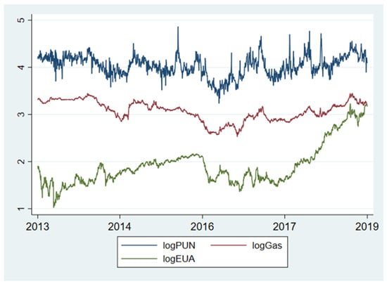
Figure A1.
Graphical representation of electricity (PUN), allowances and gas prices.
Table A1.
Summary statistics.
Table A1.
Summary statistics.
| Variable | Unit | Mean | St. Dev. | Skewness | Kurtosis |
|---|---|---|---|---|---|
| PUN | €/MWh | 57.7778 | 12.6281 | 0.5488 | 4.2116 |
| PUNp | €/MWh | 60.7118 | 14.7954 | 0.5792 | 4.3579 |
| PUNop | €/MWh | 53.8781 | 10.7104 | 0.51488 | 3.9901 |
| Gas | €/MWh | 22.0660 | 4.4279 | −0.0837 | 2.1017 |
| EUA | €/ton | 7.5589 | 4.3392 | 2.1085 | 6.7950 |
Sample period: 1 January 2013 to 31 December 2018 (1565 observations). All data are in natural logs.
Appendix A.2. Stationarity Tests
The evaluation of the interdependence between energy prices, CO2 emissions and gas prices requires a preliminary evaluation of the time-series features. In fact, different modeling strategies might be adopted depending on the stationarity properties of the observed sequences. We test if the variables of interest are non-stationary in order to exclude spurious results, through the KPSS and the ADF tests. For both tests, we perform the analysis on the series log levels as well as on the first-order difference. Results are reported in Table A2. Note that for the KPSS, the null hypothesis corresponds to the series stationarity, while for the ADF test, the null hypothesis indicates the existence of a unit root. Identifying the presence of non-stationarity in the series log-levels allows to search for cointegration relationships among the variables. KPSS and ADF tests are concordant in suggesting that the EUA and gas log-prices are non-stationary. Differently, when focusing on the electricity prices, the ADF test rejects the null of non-stationary, while the KPSS test rejects the null of stationarity. We are thus in a situation where it is not known with certainty whether the series are trend stationary or non-stationary. As our main interest is the identification of the existence of level relationships between our variables, we adopt the bound testing approach of Pesaran et al. (2001), which introduces a testing framework for identifying the presence of cointegration in cases where there is uncertainty on the stationarity properties of the series of interest. The test builds on an auto-regressive distributed lag model of the form
where yt is the dependent variable in log-levels, xt is a vector containing other variables (again in log-levels) that are potentially cointegrated with yt, and Δ denotes first order differences.
The testing procedure sequentially evaluates the null hypothesis that the lagged log-levels coefficients are jointly equal to zero, i.e., . The test statistic corresponds to a standard F-test for joint coefficient restrictions, but its value has to be compared with two bounds: if the test statistic falls below the lower bound, the variables are stationary and the procedure stops; if the test statistic is within the two bounds, the test is inconclusive and the procedure stops again; and if the test statistic falls above the upper bound, there is evidence for the existence of level relationships impacting on the first difference stationary variables. In the latter case, to exclude that the level relationships are degenerated, we test the null again with a bound approach. As in the previous case, a test statistic above the upper bound signals the existence of cointegration among the levels. Table A2 reports the results of the bound testing for several cases. Notably, in all cases, we do find evidence of long-run level relationships among the variables of interest (i.e., all test statistics are above the upper bounds—bounds are reported in the table caption). This supports our intuition about the existence of level relationships between energy prices, allowances and gas prices and justifies the use of a vector error correction model (VECM) to find a confirmation on the existence of cointegration among the variables.
Table A2.
Stationarity tests on the log-levels series.
Table A2.
Stationarity tests on the log-levels series.
| Variable | Test | Lag | Test Statistic | Lag | Test Statistic |
|---|---|---|---|---|---|
| Log-Levels | Changes in Log-Levels | ||||
| PUN | KPSS | 0.547 *** | 0.034 | ||
| PUNp | 0.463 *** | 0.030 | |||
| PUNop | 0.651 *** | 0.059 | |||
| EUA | 0.599 *** | 0.331 | |||
| Gas | 0.781 *** | 0.152 | |||
| PUN | ADF | 3 | −5.187 *** | 2 | −32.194 *** |
| PUNp | 3 | −5.387 *** | 2 | −35.453 *** | |
| PUNop | 3 | −5.378 *** | 3 | −26.109 *** | |
| EUA | 2 | 0.180 | 3 | −19.920 *** | |
| Gas | 2 | −1.826 | 3 | −19.824 *** | |
The number of lags is selected using the AIC identification criteria. The KPSS test null hypothesis is the series stationarity, while the null hypothesis of the ADF is the existence of a unit root (i.e., non-stationarity). We run the tests using a constant and a trend for the log-levels and with a constant only for the changes in the log-levels. Critical values are as follows: for the KPSS test (null rejected on the right tail, for large values of the test statistic), 0.216 at the 1% confidence level, 0.146 at the 5% level, and 0.119 at the 10% level for the case with trend, and without the trend 0.739 (1%), 0.464 (5%) and 0.347 (10%); for the ADF test (null rejected on the left tail, for large negative values of the test statistic), −3.96 at the 1% confidence level, −3.41 and −3.12 at the 5% and 1% confidence levels, respectively, with constant and a trend, and −3.43 (1%), −2.86 (5%) and −2.57 (10%) without a trend. We use stars to denote rejection of the null at the 1% level, ***, 5% level, **, and 10% level, *.
Table A3.
Bound test to cointegration.
Table A3.
Bound test to cointegration.
| PUN | GAS, EUA | 18.21 | −7.39 |
| PUNP | GAS, EUA | 16.80 | −7.09 |
| PUNOP | GAS, EUA | 20.04 | −7.74 |
The table reports several test statistics to verify null hypotheses on the bound test for cointegration. Bounds to verify the null hypotheses : 1% confidence level, lower bound (below this level, we accept the null hypothesis, and the variables are stationary), 5.15, upper bound (above this level, we reject the null hypothesis, and the variables are stationary) 6.36; 5% level, lower bound 3.79 and upper bound 4.85; 10% level, lower bound 3.17 and upper bound 4.14. Bounds for testing the null hypothesis (note that the way bounds are defined is coherent with Pesaran et al. 2001): 1% level, lower bound (below this level we accept the null hypothesis and there is no level relationship among variables) −3.43, and upper bound (above this level we reject the null hypothesis and there exist a level relationship among variables) −4.11; 5% level, lower bound −2.86, and upper bound −3.53; 10% level, lower bound −2.57, and upper bound −3.21. See Pesaran et al. (2001) for additional details.
Appendix A.3. IRFs for Model 2 and Model 3
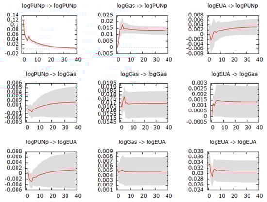
Figure A2.
Impulse response functions of the VECM model (three variables, peak PUN, one cointegration relation). The shaded area represents the 90% confidence interval.
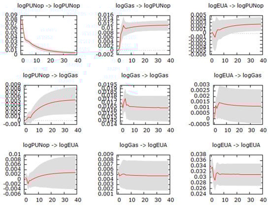
Figure A3.
Impulse response functions of the VECM model (three variables, off-peak PUN, one cointegration relation). The shaded area represents the 90% confidence interval.
Notes
| 1 | In the considered dataset, there are no negative prices, since in the MGP negative prices are not allowed. |
| 2 | Note that we are not claiming anything about the theoretical or effective efficiency of the EU-ETS allowances’ markets per se. On this topic, there exists a vast literature. See, for instance, Ibikunle and Gregoriu (2018); Hintermann (2017); and Rannou (2017). |
| 3 | See Haq et al. (2021); Khabarov et al. (2019); and Klaus (2019), for examples. |
References
- Ahamada, Ibrahim, and Djamel Kirat. 2015. The Impact of Phase II of the EU ETS on Wholesale Electricity Prices. Revue d’Economie Politique 125: 887–908. [Google Scholar] [CrossRef] [Green Version]
- Ahamada, Ibrahim, and Djamel Kirat. 2018. Non-linear Pass-Through of the CO2 Emission-Allowance Price onto Wholesale Electricity Prices. Environmental Modelling & Assessment 23: 497–510. [Google Scholar]
- Bariss, Uldis, Elvijs Avenitis, Gatis Junghans, and Dagnija Blumberga. 2016. CO2 Emission trading effect on Baltic electricity market. Energy Procedia 95: 58–65. [Google Scholar] [CrossRef] [Green Version]
- Bunn, Derek, and Carlo Fezzi. 2008. A Vector Error Correction Model of the Interactions among Gas, Electricity and Carbon Prices: An Application to the Cases of Germany and United Kingdom. In Markets for Carbon and Power Pricing in Europe: Theoretical Issues and Empirical Analyses. Aldershot and Brookfield: Edward Elgar Publishing, pp. 145–59. [Google Scholar]
- Chernyavs’ka, Liliya, and Francesco Gulli. 2008. Marginal CO2 cost pass-through under imperfect competition in power markets. Ecological Economics 68: 408–21. [Google Scholar] [CrossRef]
- Cludius, Johanna, and Regina Betz. 2020. The role of banks in EU emissions trading. Energy Journal 41: 275–99. [Google Scholar] [CrossRef]
- Daskalakis, George, Dimitris Psychoyios, and Raphael Markellos. 2009. Modeling CO2 emission allowance prices and derivatives: Evidence from the European trading scheme. Journal of Banking and Finance 33: 1230–41. [Google Scholar] [CrossRef]
- Fabra, Natalia, and Mar Reguant. 2014. Pass-through of Emissions Costs in Electricity Markets. American Economic Review 104: 2872–99. [Google Scholar] [CrossRef] [Green Version]
- Graham, Michael, Anton Hasselgren, and Jarkko Peltomaki. 2016. Using CO2 Emission Allowances in Equity Portfolios. In Handbook of Environmental and Sustainable Finance. Edited by Vikas Ramiah and Greg N. Gregoriu. Amsterdam: Elsevier, pp. 359–70. [Google Scholar]
- Haq, Inzamam Ui, Supat Chupradit, and Chunhui Huo. 2021. Do Green Bonds Act as a Hedge or a Safe Haven against Economic Policy Uncertainty? Evidence from the USA and China. International Journal of Financial Studies 9: 40. [Google Scholar] [CrossRef]
- Harasheh, Murad, and Andrea Amaduzzi. 2019. European emission allowance and equity markets: Evidence from further trading phases. Studies in Economics and Finance 36: 616–36. [Google Scholar] [CrossRef]
- Hintermann, Beat. 2016. Pass-Through of CO2 Emission Costs to Hourly Electricity Prices in Germany. Journal of the Association of Environmental and Resource Economists 3: 857–91. [Google Scholar] [CrossRef] [Green Version]
- Hintermann, Beat. 2017. Market Power in Emission Permit Markets: Theory and Evidence from the EU ETS. Environmental and Resource Economics 66: 89–112. [Google Scholar] [CrossRef] [Green Version]
- Honkatukia, Juha, Ville Malkonen, and Adriaan Perrels. 2008. Impacts of the European Emission Trade System on Finnish Wholesale Electricity Prices. In Markets for Carbon and Power Pricing in Europe: Theoretical Issues and Empirical Analyses. Edited by Francesco Gulli. Cheltenham: Edward Elgar Publishing, pp. 160–92. [Google Scholar]
- Ibikunle, Gbenga, and Andros Gregoriou. 2018. Carbon Markets: Microstructure, Pricing and Policy. London: Palgrave Macmillan. [Google Scholar]
- Johansen, Soren. 1988. Statistical Analysis of Cointegration Vectors. Journal of Economic Dynamics and Control 12: 231–54. [Google Scholar] [CrossRef]
- Johansen, Soren. 1991. Estimation and Hypothesis Testing of Cointegration Vectors in Gaussian Vector Autoregressive Models. Econometrica 59: 1551–80. [Google Scholar] [CrossRef]
- Johansen, Soren. 1995. Likelihood-Based Inference in Cointegrated Vector Autoregressive Models. Oxford: Oxford University Press. [Google Scholar]
- Jouvet, Pierre-André, and Boris Solier. 2013. An overview of CO2 cost pass-through to electricity prices in Europe. Energy Policy 61: 1370–76. [Google Scholar] [CrossRef] [Green Version]
- Khabarov, Nikolay, Ruben Lubowski, Andrey Krasovskii, and Michael Obersteiner. 2019. Flobsion—Flexible Option with Benefit Sharing. International Journal of Financial Studies 7: 22. [Google Scholar] [CrossRef] [Green Version]
- Klaus, Stocker. 2020. Financial and Economic Assessment of Tidal Stream Energy—A Case Study. International Journal of Financial Studies 8: 48. [Google Scholar] [CrossRef]
- Lo Prete, Chiara, and Catherine Norman. 2013. Rockets and feathers in power future markets? Evidence from the second phase of the EU ETS. Energy Economics 36: 312–21. [Google Scholar] [CrossRef]
- Pesaran, M. Hashem, Yongcheol Shin, and Richard Smith. 2001. Bounds testing approaches to the analysis of level relationships. Journal of Applied Econometrics 16: 289–326. [Google Scholar] [CrossRef]
- Rannou, Yves. 2017. Liquidity, information, strategic trading in an electronic order book: New insights from the European carbon markets. Research in International Business and Finance 39: 779–808. [Google Scholar] [CrossRef]
- Sijm, Jos, Karsten Neuhoff, and Yihsu Chen. 2006. CO2 cost pass-through and windfall profits in the power sector. Climate Policy 6: 49–72. [Google Scholar] [CrossRef] [Green Version]
- Sijm, Jos, S. J. Hers, W. Lise, and B. J. H. W. Wetzelaer. 2008. The Impact of the EU ETS on Electricity Prices. Final Report to DG Environment of the European Commission. ECN Report, ECN-E--08-007. Amsterdam: ECN. [Google Scholar]
Publisher’s Note: MDPI stays neutral with regard to jurisdictional claims in published maps and institutional affiliations. |
© 2021 by the authors. Licensee MDPI, Basel, Switzerland. This article is an open access article distributed under the terms and conditions of the Creative Commons Attribution (CC BY) license (https://creativecommons.org/licenses/by/4.0/).