Artificial Intelligence Approach to Momentum Risk-Taking

Abstract

We propose a mathematical model of momentum risk-taking, which is essentially real-time risk management focused on short-term volatility. Its implementation, a fully automated momentum equity trading system, is systematically discussed in this paper. It proved to be successful in extensive historical and real-time experiments. Momentum risk-taking is one of the key components of general decision-making, a challenge for artificial intelligence and machine learning. We begin with a new mathematical approach to news impact on share prices, which models well their power-type growth, periodicity, and the market phenomena like price targets and profit-taking. This theory generally requires Bessel and hypergeometric functions. Its discretization results in some tables of bids, basically, expected returns for main investment horizons, the key in our trading system. A preimage of our approach is a new contract card game. There are relations to random processes and the fractional Brownian motion. The ODE we obtained, especially those of Bessel-type, appeared to give surprisingly accurate modeling of the spread of COVID-19.

1. Introduction

1.1. Objectives and Tools

We propose a new theory of momentum risk-taking, which is basically real-time risk management, one of the key components of general decision-making. We focus on momentum risk-taking, MRT, when the decisions must be fast and mostly short-term. This is a development of “thinking fast” from (Kahneman 2011). Applications to stock markets are key to us; a new approach to short-term volatility and high- frequency trading is the main theoretical result of this paper. Its implementation is a momentum trading system, which was extensively tested in stock markets, including real-time trading. The discussion of its performance is an important part of the paper. Stock markets provide a unique opportunity to test our theory, but the core mechanisms of MRT seem quite universal. We will argue that MRT is a major component of any intelligence. Our results indicate that modeling such mechanisms is within the reach of artificial intelligence systems; they can be natural “ends” and also indispensable research “means”.

The key components are our new continuous mathematical model of news impact on share prices and its “stratified discretization” necessary to deal with discontinuous functions and different investing horizons. Basically, the spread of news for a single event is $t^r$ in terms of time $t$ with fractional powers (exponents) r multiplied by proper functions in the form $cos(Alog(t))$. The $log(t)$-periodicity here resembles that of Elliot waves. The refined version of the corresponding ODE requires Bessel functions. It gives the t-periodicity, modeling profit taking. Understanding profit-taking is of obvious importance in the theory of market volatility (see, e.g., Andersen et al. 2017; Engle and Ng 1993; Fouque and Langsam 2013; Fouque et al. 2003; O’Hara 2015). Hypergeometric functions naturally occur when the impact of two events is considered, which is related to certain types of hedging.

Power-laws. The power laws for price functions are fundamental in Econophysics. The so-called efficient market hypothesis and similar approaches are essentially based on the assumption that returns follow the normal distribution. This contradicts the behavior of modern markets, especially short-term fluctuations of share prices. The power-law hypothesis is much more suitable for this; see, e.g., (Mantegna and Stanley 2000). There are various market processes beyond the power-law, but this is basically sufficient; see, e.g., (Gubiec et al. 2012).

Power-laws are quite natural for almost any physics approaches, well beyond stock markets. They serve quite a variety of different economics areas, which was convincingly demonstrated in (Gabaix 2016). A starting point for us is that they describe very well news impact and momentum risk-taking, MRT. Their origin in Behavior Science and Behavior Finance is significant in this work.

From this perspective, it is not very surprising that the systems of differential equations we obtained for share prices appeared applicable to model the spread of COVID-19 in many countries and for various waves of this pandemic. To be more exact, the two-phase solution proposed in (Cherednik 2020), matches very well the curves of total numbers of detected infections, practically without exception. Let us provide some detail.

The first phase is modeled by Bessel functions. Systems (14) and (15) are used, where c is the transmission rate and e the intensity of protective measures. The second phase is described by systems (14) and (15). Both are of power-type and have some saturation. The saturation and related periodicity are of course more difficult to observe in the stock markets due to the constant stream of market related news and high volatility. This is different for epidemics; the usage of Bessel functions was convincingly confirmed for COVID-19. The accuracy and the uniformity of our ODE appeared well beyond what anyone could expect for epidemics.

The power-law of epidemics contradicts the usual SIR-type models, which are based on the assumption of the exponential growth of the number of cases unless under the herd immunity. With COVID-19, the exponential growth, if any, can be observed only during very short initial periods (never during the middle stages). This is discussed systematically in (Cherednik 2021).

Discretization. As with any theory, our one must be checked experimentally. Stock markets are the main examples for us; they are quite a test for any risk-management theories. An obvious problem is that stock charts are discontinuous, so differential equations must be generally replaced by difference ones. Novel approaches to the discretization appeared necessary; cf. (Cheridito and Sepin 2014). We restrict ourselves with relatively short time periods after the event; the high volatility right after the news is mostly avoided. Then the core of our approach is the usage of tables of bids, which is essentially a ranked collection of sample time-forecasts for different time-horizons.

Given a chart, these tables provide a short-term prediction of its evolution, which extrapolate the prior behavior in some “non-linear” way; cf. (Guéant 2013). Forecasting here is not on the basis of derivatives of price-functions or their difference counterparts, though they are employed too. This is quite a non-linear process, which includes various time-horizons. Our approach actually reflects the ways our brains work.

Our tables of bids are similar to bidding tables in contract card games, though the role of time, the non-linearity of our tables, and some other features have no counterparts with cards. In the realm of stock markets, the tables help to determine the proper time-horizons: optimal durations of the investments. Basically, this is short-term forecasting the share prices based on auction-type procedures. We think that our brain “employs” similar procedures for risk-taking, so the usage of such bidding tables can be quite universal, well beyond playing cards and trading stocks.

Risk-taking. The standard approach to understanding the ways our brain works is via carefully designed experiments, which are mostly focused on very basic tasks, which are mostly very simplified and sometimes artificial. However, the simpler the challenges the more special and primitive tools our brain invokes. This means that laboratory experiments can generally clarify only very basic features; they are games in a sense. With any game, our brain readily switches to the corresponding optimal thinking mode, at least upon some training; we are good with this. Therefore, the experiments mostly measure our ways to play very specific “games”, which is insufficient to understand what is general purpose AI. The risks must be as real as possible to force our brain to use its full potential, which is hardly possible in experiments. Real behavior from people is difficult to recreate in artificially designed situations, even well crafted.

It seems that the most promising, if not the only, rigorous approach to understanding risk-taking and other processes of this kind is to do our best with creating artificial intelligence systems and then comparing their decisions in real situations with those of people. Of course, the aim here is to improve our decision-making, but any “simple” reproduction of our real behavior is of course a breakthrough of a great scale.

Toward AI systems. The automated momentum trading system based on our approach can be seen as a step in this direction; it is discussed in the second part of this paper. Its preimage is a new contract card game presented at the end. By design, our trading system uses only the changes of share prices; i.e., it operates only on the basis of the technical analysis. So it is inevitably “late” with any decisions vs. professional traders and investors, and is subject to the bid-ask spread and many other factors reducing the profitability. In spite of such disadvantages, the system proved to be profitable, which is some justification of our approach.

We discuss the main features of our trading system in the paper and provide some typical results of its performance. Designing historic experiments is always a very serious problem: the usage of any kind of “future” must be fully excluded. The real-time trading is an ultimate test: the system was tested systematically (with about 1000 companies). The results we provide can supply those who will try to follow our approach and implement our tables with some benchmarks. We think that the pont-tables from Section 4.3 can significantly help to get used to the 2-bid tables from Section 3.3.

Importantly, we can always “explain”, interpret to be exact, the trades our system makes. Our system is not a black box; its risk-taking preferences can be seen. In a sense, it is a quantitative model of “thinking fast” from (Kahneman 2011). Indeed, traders must promptly react to many unknown factors, which is based on some special market intuition. The latter must be of obvious interest to cognitive theory and behavioral finance.

1.2. Organization of the Paper

Here, in the Introduction, we describe our approach and discuss its general origins, including risk-management and some aspects of cognitive theory. Momentum risk-taking is essentially short-term forecasting based on the current information (frequently incomplete). We demonstrate that it can be modeled mathematically. Due to our focus on professional trading, we disregard the expected utility hypothesis originated by Daniel Bernoulli, the asymmetry between loss and gain from prospective theory, and similar aspects. The market agents are assumed to act “rationally” on the basis of the current news impact: the purpose of our AI system is to capture their preferences.

Section 2 presents our mathematical model of market news impact, based on systems of differential equations resulting in Bessel functions, hypergeometric functions, and their degenerations. These systems are closely connected with new tools in harmonic analysis and random processes, namely, with the Dunkl eigenvalue problem (see, e.g., Opdam 1993; Cherednik 2005) and Macdonald’s processes (Borodin and Corwin 2014).

As a demonstration of the universality of our system, we show that it models well the tree growth in a difference setting and provide other examples.

The connection with fractional Brownian motion (fBM) is briefly discussed at the end of Section 2.4. Our price-functions are related to the standard deviations and transition probability densities of the corresponding processes, which provides a statistical framework for our approach. See (Cheridito 2001; Gatheral et al. 2018; Guasoni et al. 2017; Bouchaud 2001) concerning fBM in studying market volatility and power-laws for price functions. See, also, (Mantegna and Stanley 2000; Gabaix 2016; Gubiec et al. 2012) on the power-laws in econophysics.

Using a single fBM with a small Hurst exponent as a model for a price function creates a theoretical problem with the existence of arbitrage (some kind of “free lunch”) due to the negatively correlated increments. However, mixed fBM are arbitrage free, and we are using only relatively short time-intervals, where this concern is not quite relevant. The author thanks Patrick Cheridito for a discussion.

We mostly consider the impact of one-two events. Statistical ensembles of news are mathematically significantly more challenging. The corresponding stochastic processes are similar to those in (Borodin and Corwin 2014). Our trading system provides experimental support for our approach mostly within modeling the impacts of isolated consecutive events. The “multi-dimensional” theory of ensembles of events is generally doable mathematically but seems really difficult to check experimentally in real markets.

Section 3 contains a reasonably complete description of the algorithms of our trading system. The results of extensive experiments, including real-time trading, serve two purposes. First, we provide evidence for power-laws for price functions with exponents depending on the investment horizons (say, it can be $0.137$ for day-trading).

See here (O’Hara 2015) concerning general aspects of high-frequency market micro-structure and its effect on the strategies of traders and markets. Another study, (Brogaard et al. 2014), contains a general discussion of the price movements for high-frequency trading and the role of horizons.

Let us mention that there are various models that distinguish between informed and uniformed traders, for instance, the Kyle model and the Glosten-Milgrom model from (Glosten and Milgrom 1985). They are important to understand the bid-ask spread. The assumption is that the price schedule is linear, different to our power-growth hypothesis. We do not follow this way, but significant changes of prices are the main trading signals for us.

Second, we provide some performance benchmarks for those who may follow our approach in their own trading systems. Our system has many new features, including the simultaneous running of its multiple variants (sometimes even with identical opti-parameters but with different entry points), simultaneous pro-trend and contra-trend trading, the usage of the results of optimization for creating weights of companies, and so on. Potential followers must know what to expect, theoretically and practically. We also explain how testing the system was performed.

We do not discuss much the machine learning procedures we employ, namely the optimization of parameters and creating the company weights. The discretization parameters, counterparts of action potentials for neurons, are the key for us, but there are also important difference counterparts of first and second derivatives for the charts we use for forecasting and trading. There is vast ML literature on entropy, information theory, Bayesian predictive method, and generative adversarial networks, GAN. The latter approach is somewhat similar to our auction-type procedure, when different decision-making “bids” from different investment horizons contest with each other; (cf. Delpini and Bormetti 2015; Ho and Stefano 2016). See also (Sirignano and Cont 2019) about some general perspectives of deep learning.

Since we deal with a limited number of opti-parameters (all of them have theoretical meaning), a relatively straightforward gradient method is mostly used for the optimization. It is rare when our AI system cannot find the parameters providing a solid jump in performance for almost any “education periods”, though their uniqueness is of course not granted. This is for individual companies or for portfolios. The weights of the companies we use are based on the results of prior optimization. We omit the discussion of the usage of correlations between equities in this paper, which is common in automated investing systems. This is present in our system, but mostly via creating some clusters of companies/equities to be traded under the same opti-parameters. The impact of our optimization-based weights can be significant, but using them generally restricts the trading volumes, which is a consideration for us.

Section 4 is exceptional. We motivate our 2-bids by designing a contract card game, pont, combining the elements of bridge and poker. It adds poker-style uncertainty to the bridge-type auction. The contract is declared on the basis of six cards, but the hand can consist of up to nine, which is determined by the declarer, the winner of the auction. The flexible size of hands is a counterpart of time-horizons. Thus, we add poker risk-taking to bridge-type bids, which is similar to 2-bids in our trading system. It appeared that the players can easily get used to such “fractional bids”; the size of the hand is the denominator. It is closely connected with our approach to discretization and actually models that in neural networks. Our 2-bids are discrete, though the threshold is subject to their optimization. The play (taking tricks) has almost nothing to do with stock markets: pont is just a game. However, its role as the justification of bids is quite similar to markets. The bidding is sufficiently non-trivial in pont; we consider it a good model of real risk-taking. The play (the process of justification of the bids) is missing in poker.

1.3. AI and Risk-Taking

The purpose of artificial intelligence (AI) systems is to perform tasks that require human cognition. Actually, the aim here is to exceed human decision-making abilities using computers and machine learning. Even if the quality of automated decisions is mediocre, the cost efficiency, speed, and the broad range of applications can be “superhuman” and result in great societal and economic benefits. There is a lot of progress with narrow AI, focusing on special tasks. However, we are decades away from general purpose AI according to the conclusion from “The National Artificial Intelligence Research and Development Strategic Plan (2019 update)” by the National Science & Technology Council (USA). The astonishing versatility and flexibility of human intelligence remains quite a challenge, and not only because our brain contains about 100 billion neurons.

Decision-making is the key test for any AI systems. This is quite a complex process. Risk management is one of its important components, which generally requires an ample system of protection measures aimed at reducing future risks. The focus of decision-making is generally on the latter, not on exact timing. The prediction of earthquakes is an example: we almost never know in advance when they might occur. For us, risk-taking is a permanent process of corrections, including the termination of unsuccessful positions and opening new ones. See, e.g., (Fouque and Langsam 2013) for various aspects of risk management, including high-frequency trading, and (Engle and Ng 1993) for some mathematical aspects.

Momentum risk-taking can be then broadly defined as real-time risk management, which includes prompt responses to any events and developments and short-term forecasting. This is momentum, but a lot of prior knowledge and experience is needed; see, e.g., (Engle and Ng 1993). The events we are reacting to are mostly not of a brand new type; almost always, similar ones occurred before. The problem is to address quickly their type, strength, and other factors involved. Real-time monitoring of the developments before and after the decision is an important part of risk-taking. The action can be required immediately, so it can be difficult to understand what really affected our decision. Kahneman’s “Thinking fast”, intuition, subconscious processes are certainly involved. Though this can be not too transcendental: we switch to a special mode of our brain for fast managing time-sensitive information.

Such “momentum” (sometimes subconscious) processing the signals can be not very different from the usual (systematic, rational) one, but it is with many simplifications. AI can be relevant here. Moreover, AI can help a lot to understand which kind of “thinking fast” and “intuition” is used; this alone is quite a motivation of the present paper and our project. One of our main observations (based on machine modeling) is that core risk-taking is actually controlled by very few parameters. Moreover, these parameters seem to be of universal nature, though they are obviously adjusted to concrete situations.

The broad nature of risk-taking can be seen in stock markets. For instance, the results based on the optimization of individual companies are only somewhat better than the results based on the optimization performed for the portfolios of companies. Generally, the greater variety of different risk-taking tasks someone went through, games included, the greater someone’s risk-taking skills. This sounds quite obvious but is very difficult to implement in any automated systems; developing general purpose artificial intelligence systems is needed here, not just those focused on specific tasks. We mention (Buchanan 2019) that contains an extensive list of references on AI in finance and a timeline (from 1937). See also recent (Novak et al. 2021) for some other aspects.

1.4. Universality of MRT

Let us try to outline minimal tools that seem necessary for any risk-taking. This will be not a biological (neuroscientific) or philosophical discussion. Our approach is actually via mathematical universality of the corresponding differential equations.

Our brain does many things; decision-making is one of the keys for any intelligence. Though the latter is, of course, much broader. Science is an example of “broad intelligence”. However, even very abstract research directions involve risk-taking: the evaluation of the importance, the choice of methods, expectations, and so on. Games are examples of “abstract activities”, but they serve a clear purpose of developing and training our decision-making abilities (social skills included).

With this understanding of momentum decision-making, there must be no significant difference between humans, other creatures, and artificial systems. Instincts and reflexes are important here, but this a rational and uniform process. Our ability to plan long-term is of course a cultural phenomenon; this requires a concept of time and many intellectual abilities. Generally, long-term forecasting and planning seem beyond what AI can be expected to do, especially with the processes of high uncertainty.

However, mathematical modeling seems doable for small periods under momentum risk-taking, for short MRT. Almost any creatures have some basic concepts of time, at least short-term, sometimes at the level of chemical and physical processes. The results of MRT can be clearly seen and the corresponding learning process must be universal.

It is not impossible that the core mechanisms of MRT can be observed in the neural architecture of our brain. One of the main mechanisms is the well-studied action potential; its counterparts are the key for the discretization in this paper. The action-type procedures between different options are obviously present in our brain, too. Mathematically, any decision making must require some price-functions. It is, of course, a great challenge to understand how such functions can be formed and “stored” in our brain.

Basically, MRT is news-driven short-term forecasting and the corresponding risk-taking. Our brain does a lot of things; e.g., about 50 percent of the cortex is doing vision. MRT is about a very exact segment of its activities: fast analysis of new events.

After information reaches the level of news by our brain (which itself is quite a process), the process of its initial classification begins, including its rank, weight, etc. The weight is, of course, based on prior experience and “deep learning”.

We demonstrate that the differential (or difference) equations must be for the news-function (the spread of news) combined with the price-function. For modeling epidemics in (Cherednik 2020, 2021), the active management plays the role of the price-function; the match with the waves of COVID-19 appeared to be almost perfect.

For brain processes, the news-function basically measures the resources (the number of neurons) currently involved in the analysis of an event. The price-function provides expected importance of this particular event vs. other events and the corresponding expected brain resources needed for its analysis. The latter can be increased or diminished in process, depending on the news-function. For instance, the “price of news” will increase when the news generates neural activities greater than expected. When the current number of neurons involved approaches the levels provided by the price-function, the news “fades”. Its impact can still continue to grow, as well as the price-function, but the brain will then attempt to reduce the resources used for its analysis.

This sort of interaction is essentially the system of differential equation we suggest, which can be solved in terms of power-type functions and Bessel functions. We expect that such 2-function “interaction”, the actually needed resources vs. those expected to be used, is present in almost any MRT. The simplicity and fundamental nature of the corresponding differential and difference equations is a strong (mathematical) confirmation. These equations are relatively new, though with very strong connections with classical special functions. Nonsymmetric Bessel functions, Dunkl operators, and other recent tools in harmonic analysis are involved here (in dimension one).

An example: driving. Brain activities while driving a car provide a convenient example of “general” MRT. Permanent visual information and a lot of similar information is a must here for MRT. Obtaining and processing such information is very resource consuming, much greater than MRT itself.

The actual beginning of MRT is when our brain identifies events. They can be conditions of the road, especially those requiring special attention, road signs, pedestrians, neighboring cars, navigation matters, and so on; see, e.g., arXiv:1711.06976, arXiv:1906.02939 on self-driving cars. Importantly, all such categories of potential events are supposed to be analyzed constantly and simultaneously, even if the current news is in one particular category. There is an almost exact analogy with trading stocks, especially when they are treated independently, the main regime for our trading system: all stocks considered for potential investing and investment horizons must be constantly monitored, regardless of the current or expected positions.

Only some events will reach in our brain the level of signals. The separation of the signals from noise is quite a problem, which requires a lot of prior experience. By noise, we mean “insignificant events”, those that hardly require special consideration. After the signals are determined, our brain is supposed to estimate the resources needed for the analysis of the signal. This stage requires invoking from the memory the average cost of the analysis of similar events, which is essentially an estimate for the expected brain resources (neurons) needed for its analysis. The “cost-function” replaces here the “price-function” $p(t)$ for stocks.

Then a systematic analysis begins, which can trigger the number of neurons significantly different from what was initially “allocated”. This can be because of unexpected complexity of the event, due to changing its priority for driving, and so on. When the “cost” of the activity becomes beyond projected cost-levels, our brain will automatically attempt to reduce the number of neurons involved.

The risk-taking in this example is a combination of such analysis with the corresponding driving decisions. The latter must be obviously fast. The rank (category) of the news and its “intensity” must be high enough to enter and then win the “action”, which is similar to our 2-bids.

The general assumption is that short-term event impact is of power-type with some fractional exponent. Our brain (conjecturally!) constantly produces short-term predictions for the importance of the event, some “termination curves” of power-type in terms of t. They are used to end or restrict our analysis when the importance of the current event (measured by our brain) becomes under such a curve. The “final cost” of the performed analysis reflects its current importance and may influence the general weight of the corresponding type of event; it will be then stored in our memory in some form (presumably).

1.5. Games as Concepts

AI systems do not always follow the ways of our brain, even if the problems are human-related. However, nature, our brain included, is definitely the prime source of concepts for any AI. Just to give an example, airplanes are very different from birds, but the concept of flying is from nature. This is no different for AI. Narrow AI systems, in specialized well-defined domains, can sometimes follow “non-human”, ways. However general AI systems are expected to borrow a lot from human intelligence, though the final implementations can be quite different: “aircrafts vs. birds”.

Importantly, many faces of decision-making are reflected in the games we play. Some include timing, some do not. For instance, solving puzzles and playing chess are not focused on timing, unless in tournaments. On the other hand, poker and contract card games are time sensitive. The interaction and risks in card games are as close as possible to real life, for models of course, which they are. Investing is obviously closer to playing poker than to playing chess or bridge. Poker’s bidding is a great model of dealing with uncertainties, but the risks are too “mathematical” and the actual “play” is missing. Solid rules and protocols make the stock market some kind of a game, but here the risks are (more than) real. From this perspective, it provides a highly developed and quite universal “model” of risk-taking, which is of obvious interest.

Psychologically, games reflect life in various ways, potentially preparing us for real-life challenges; we discuss “intellectual games”. Some are designed to deal with real tasks; playing them can be more dangerous than life itself. Using game theory, especially mean field games, is quite common in financial mathematics; see, e.g., (Guéant et al. 2011). We found no card game reflecting our concept of momentum risk-taking and invented a new one, pont, which is essentially a version of bridge with poker-style bidding.

Stock markets by design mean that their “agents” look only to their own interests and to market prices (Guéant et al. 2011), though investing is a complex and very much interactive process with solid grounds in our psychology. As such, investing is a great confirmation of the universality of momentum risk-taking, MRT. It looks like there is some general purpose risk-taking source code in our brain in charge of all kinds of momentum risks, which constantly improves itself whatever the nature of the risk and uncertainty. If this is true, then we can try to use AI to understand this code and to model it!

Philosophically, we test here Kant’s antinomy 2 (atomism), by considering risk-taking as a composite substance, and his antinomy 3 (causal determinism) concerning the flexibility of decision-making. We study the stock markets as “an end in themselves”, disregarding their economic and societal purpose for the sake of mathematical modeling.

1.6. Momentum Investing

Marshmallow test. A well-known test for children, “one marshmallow now or two in 15 min”, is actually one of the origins of our modeling risk-taking in stock markets. The latest psychological experiments found limited support to the thesis that delayed gratification with children leads to better outcomes in their futures (Watts et al. 2018). “Two in 15 min” can be simply because a child already learned that “patience is rewarded”. The 15 min interval can also be not that short for little ones. Then the impatience depends on the age, social and economic background, etc. Some can simply favor short-term solutions. If the interval increases (say, days) or the reward is diminished, the “impatience” can be well justified. This means the problem is actually quantitative.

Similar to (Kahneman 2011), we began with some analysis of psychological roots. A starting point of our research was a postulate that we have quite a rigid “table” of risk preferences in our brain. To give a simple example, if the return was 1% today and you can count on an extra 1% tomorrow, then do not sell. However, if “only” 0.5% can be expected tomorrow and even this is not granted, then probably sell now and avoid extra risks. Basically, with 2% for 2 days, we would wait, but with 1% for 2 days, we certainly sell, because we have already made 1% for 1 day. Presumably, our brain takes the average here, which makes 1.5% tomorrow a “reasonable compensation” for the delay. This is ignoring the risks and uncertainty, which are always present and influence decision-making.

The auction in pont does almost exactly this. For instance, the smallest bid during the auction is $3/6$ (3 from 6), which means that you are obliged to take 3 tricks with 6 cards (your initial hand), or, upon the “increases”, 4 from 7–8, or 5 from 9 (requesting up to 3 additional cards). So the pont-bids are actually fractional; the next bid is $4/7$, where your contract (if you win the auction) must be $4/6,4/7,5/8$, or $6/9$. The number of cards in your hand and the number of taken tricks reflect respectively the duration of the investment and the return.

The play itself (the process of playing) is of course not market-related; this is simply a way to validate your bid. In real investing, the “contract” means opening a position and the “play” is finding the moment of its termination. The resulting return is similar to the value of the contract. There are many successful ways to invest; picking one of them resembles very much bidding in card games, but “timing” is not well reflected in card games. Pont somehow addresses this; it is a model of our approach to comparing returns for different durations of positions. Comparing different horizons is not something unusual for our brain. Interesting mathematics is involved here, including Bessel and hypergeometric functions.

Stock markets are, of course, much more sophisticated than this. For instance, the execution risks are connected with the investment risks (Engle and Ferstenberg 2007). Also, opening short positions and terminations of long ones are frequently based on the same sell signals, so they are related. Mathematically, pont-bids are linear; the tables of bids we use in our trading system are nonlinear. Though the similarity is strong.

Market implementation. The termination rules we use are based on termination curves. These curves are directly linked to forecasting share prices. The hierarchy of basic pont-bids discussed above is such a curve (with 4 points): 3 tricks from 6 cards, 4 tricks from 7 or 8 cards, and 5 from 9. As with cards, the discretization of stock market bids is necessary for our trading system to work. The separation of the signals from noise, which we do successfully, absolutely requires such a discretization. Stock market charts are discontinuous functions by their nature, especially short-term. The discretization of bids is also closely related to the discretization of time, which is inevitable for finding the optimal time range of investments (in hours, days, weeks).

We will argue below that the prediction and termination curves are of type $const·t^r$, where t is time and r is some fraction (generally, below $1/2$). This assumption matches well momentum investing, which can be defined as “investing on news”. It works well for individual companies, portfolios of companies, market indexes, including SPY, the spider, and for commodities; it seems to us of quite general nature.

We note that the optimization becomes significantly more involved for our trading system when strict hedging was imposed, i.e., when for any open position, an equal amount is invested in the opposite direction in SPY or similar; see (Bouchard et al. 2018). Theoretically, hypergeometric functions are needed here; using $\left\{t^r\right\}$ becomes too approximate. The system worked, but the returns were less impressive. More generally, the correlations between companies are important; this is beyond the system we present, though we did the group optimization.

In our approach, we do not even try to evaluate the news itself. Its impact is measured through the response of the markets via stock prices and trading volumes. Thus, the parameters we find and use actually reflect investor risk-taking preferences, which can be expected sufficiently stable. The trading frequency is one of the main factors here; see for instance (Almgren 2012; Cheridito and Sepin 2014; Chan and Sircar 2015). The risk preferences of day-traders are quite different from those of mutual funds. The challenge is that a stock can be involved in trading with different frequencies and horizons, which was addressed in our bidding tables. This is especially applicable to trading indices; see, e.g., (Fouque et al. 2003; Guasoni et al. 2019). All kinds of trading patterns are present for SPY, and our system mostly managed them well. See (Bouchaud 2001; Delpini and Bormetti 2015) on using typical time scales.

The design of our trading systems includes many special market twists. For instance, the counter-trend (contrarian) variants of our trading system frequently outperform pro-trend ones. We actually used both variants simultaneously, which is some kind of hedging. Contra-trend trading can be successful because of several reasons. Our system needs time to measure the impact of the news to be sure that this is not “noise”; large trade sizes are a consideration too (see Gökay et al. 2011). Counter-trend trading is not unusual in stock markets (Conrad and Kaul 1998). Let us mention here that the initial version of our trading system mostly relied on the intersections of termination curves with actual charts, changing the directions of positions correspondingly. It worked reasonably, but reacted slowly to fast market moves, which was improved via “start 2-bids”, where we used the same curves to produce signals for opening new positions; this complemented well our usage of the intersections.

To trade real-time, our system was designed completely automated, a must for any AI even if they are used interactively. See (Cartea et al. 2015) concerning various aspects of automated high-frequency trading. We note that the trades of our system are fully explainable; it is not a “black box”. Only such AI can be really trustworthy; see, e.g., (Horel and Giesecke 2019).

2. Modeling News Impact

In this section, a simple mathematical model of short-term impact of news is suggested. News-driven fluctuations of share prices are the core examples. We come to certain linear differential equations, which can be generally solved in terms of hypergeometric functions. We focus on elementary solutions only. They have market applications, which were extensively tested in various stock markets, including real-time experiments. There is another way to obtain essentially the same equations via random processes, but it will not be touched upon in this paper. See (Engle and Ng 1993); e.g., compare their News Impact Curves with our ones.

2.1. Hierarchy of News

Let us briefly describe the types of company or industry news, which can be primary and secondary. The primary ones are basically core events and announcements. For instance, (a) new products or acquisitions, (b) significant changes of earning estimates by the company, (c) upgrades or downgrades by leading market analysts. Major sector, industry, or economy news are of this kind, too.

Almost any core news generates a flow of secondary news in the form of (highly correlated) reports, reviews, and commentaries. They mostly present the same core news, but sometimes can impact our behavior even greater than the original event. In our model, commentaries will be generally treated on equal grounds with the core announcements.

By reports, we mean analysts’ reports on the core event including perspectives and predictions. Then reviews collect and present the main findings in reports, mostly aiming at professional investors. Finally, the news itself and the findings above reach all consumers via mass media mostly in the form of commentaries.

Importantly, consumers will be influenced by all primary and secondary news more or less regardless of the level, the “distance” from the actual event. The actual originality is not the point here. So the impact of the commentaries can be significant and quite comparable with the impact of the event itself.

The Basic Equation

We assume that the impact of an event at the moment t is proportional to the t-derivative of the total number of pieces of news reflecting the event after it and before t. The coefficient of proportionality $0<c\le 1$ will be called the reduction coefficient; it depends on time, but mostly it will be treated as a constant.

The value $c=1$ can be reached right after the news, and then c tends to 0 with time, depending on the “investment horizon” (hours, days, months); cf. (Delpini and Bormetti 2015). Let us comment on this. Generally,

(i)

analytic reports and all secondary news tend to soften the expected implications of the core news,

(ii)

commentaries of all kinds disperse the original core news and diminish the expectations even further,

(iii)

the longer time passes after the core event and the core news, the smaller their impact becomes.

All three mathematically mean that the coefficient c approaches zero as $t\to \infty .$ Indeed, putting news into perspective is the purpose of analysis and commentaries, but this almost always reduces the original expectations. In momentum investing, the impact of news fades faster for short-term investing vs. long-term. Approximately, if the trading positions are in days or weeks then $c\sim 1/2$ can be expected vs. $c=1$ for months; it can be significantly smaller for high-frequency trading. Our tables provide some “natural” c-coefficients for different trading frequencies, investment categories.

From now on, news will be represented by a positive or negative real number, i.e., we assign a numerical value to it. Also, we assume that the time distribution of news is essentially uniform in the following sense.

Let $N(t)$ be the total sum of news values (positive or negative numbers) released from 0 to moment $t.$ Then the number of pieces of news (their total value, to be exact) arriving from t to $t+\delta$ for some $\delta$, i.e., $N(t+\delta )-N(t),$ equals approximately $c·\delta ·N(t)/t,$ which is $\delta$ times the reduced average of all previous news from 0 till $t.$ The greater the intensity (time-density) of commentaries, etc., triggered by an event, which is $N(t)/t$, the greater the number of new commentaries. We come to the following differential equation:

$$\begin{array}{cc}\hfill & \frac{dN(t)}{dt}=\frac{c}{t}N(t).\hfill \end{array}$$

(1)

It can be solved immediately if c is a constant: $N(t)=A{t}^c$ for a constant $A>0.$ When $c=1$ the growth of $N(t)$ is linear, i.e., the event does not “fade” with time and continues to attract constant attention. We disregard that $N(t)$ can be bounded; adding the “saturation” will be addressed later. A physics-style argument in favor of this equation is its self-similarity: the solutions are multiplied by some constants when the time units change, and c does not depend on the choice of units.

Tree growth. Equations of this type can be expected to have many applications. Let us give one example. We will switch to a difference counterpart of (1), naturally adding minimal “maturity”:

$$\begin{array}{cc}\hfill & f_n-f_{n-1}=\frac{c}{n-2}{f}_{n-2}-\lambda f_{n-1}\mathrm{for}n>2,\lambda \ge 0.\hfill \end{array}$$

(2)

when $\lambda =0$, this is a variant of the famous Fibonacci recurrence with the birth rate $\frac{c}{n-2}$, i.e., when it is inversely proportional to “time”. The term $-\lambda f_{n-1}$ here restricts over-population by allowing “emigration”.

Setting $\lambda =0,c=1,$ the fundamental solutions are: $f_n^0=n,f_n^1=D_n/(n-1)!$, where $D_n$ is the number of n-derangements, permutations of n elements without fixed elements. The second solution approaches $n/e$ as $n\to \infty$, so both have linear growth at infinity. We argue that $f_n$ in (2) basically describes the height of a tree at its nth year.

In contrast to the “Fibonacci rabbits”, trees grow linearly at most. The corresponding $f_n-f_{n-1}$ is proportional to the corresponding $f_{n-2}$, where the coefficient of proportionality, “the birth rate”, is roughly the surface area of the root system divided by the volume of the tree, i.e., it is qualitatively $r^2/r^3=1/r$. Then we take the “radius” of the tree r proportional to n. It is directly correlated with the number of tree rings and is approximately about the same for the tree and its root system. We obtain $\frac{c}{n-2}$. This can be somewhat similar to the growth of neuron nets in our brain. Providing the potential for the peripheral area of the existing net must be sufficient to keep the whole net active. So the rate of change is vaguely inversely proportional to the radius, which we make t, assuming that the total electric charge (“nutrition”) that can be used for this particular net is limited.

Making $c\simeq 1$ corresponds to the “middle stage” of tree growth. In the beginning, the volume of the tree is $r^2$ rather than $r^3$, so the tree can grow exponentially for a short period of time. Only the “active part” of its root system contributes to the growth, which eventually diminishes $r^2$ to r or so. This gives the term $\frac{c}{{(n-2)}^2}{f}_{n-2}$ in (2) and results in the saturation of the tree size at the late stage of its life cycle, which matches real tree growth. This is parallel to the fact that the reduction coefficient $c$ for $N(t)$ tends to 0 when $t\to \infty$.

There are obvious differences between news impact and tree growth. For instance, adding $-\lambda f_{n-1}$ is secondary for trees (due to their aging or similar growth reductions), but this term is of fundamental importance for the news. It reflects “pricing news”; see Section 2.2. Surprisingly, such different processes are quite similar mathematically, which clearly indicates that (1) and (2) are of universal nature.

Without going into detail, let us mention that solving (2) and similar difference Dunkl-type equations generally requires basic (difference) hypergeometric functions and their variants. This is actually a relatively recent direction; see, e.g., (Cherednik 2005).

2.2. Adding Price Targets

So far, we have not considered the following market-style response to news: when the news is already priced in, i.e., the current share price already includes it, the effect of further (secondary) news goes down. Similarly, when the stock is considered underpriced, positive commentaries have a greater impact. There is a specific market way to address this: upgrades and downgrades. They generally set new share price targets. The main difference here from general news is the dependence on the current share price. Generally, upgrades, are all market, company, or equity news of any levels addressing (depending on) the share prices.

Similar to $N(t)$, we represent upgrades by positive or negative numbers, using the notation $U(t)$ instead of $N(t).$ Thus $U(t)$, the sum of values of upgrades, depends on the share price. The following normalization $u(t)=U(t)/U(0)-1$ will be convenient below.

Let $P_t$ be the share price and $p(t)=(P_t-P_0)/P_0$ be the rate of return from the price-level $P_0$. The equation above must be corrected for $u(t)$, since $U(t)$ goes down if the share price “sufficiently” went up after the event, i.e., the news is already priced in. Similarly, it goes up if the stock is considered undervalued. This correction can be assumed proportional to $p(t)/t,$ the average rate of change of $p(t)$ from 0, which is more “balanced” vs. taking $dp(t)/dt$ here. Thus we arrive at the differential equation:

$$\begin{array}{cc}\hfill & \frac{du(t)}{dt}=\frac{c}{t}u(t)-\frac{1}{\sigma t}p(t).\hfill \end{array}$$

(3)

We note that the term $p(t)/t$ can be replaced by “more aggressive” $p(t)t^{\nu -1}$ for $0<\nu \le 1$; see system (20) and (21) below. For instance, it means for $c=0$: the longer $p(t)$ grows as $t^{\nu -1}$, the greater the number of downgrades. i.e., $p(t)\approx \mathrm{Const}{t}^{1-\nu }$ is considered non-sustainable.

We will switch from now on from $N(t)$ to $u(t)$. Here $\sigma$ is qualitatively proportional to the $P/E$ or $P/S.$ More generally, it reflects the expected growth of the company. Mathematically, $\sigma$ is essentially as follows.

Let us assume that $p(t)$ is basically linear in terms of t and “shift” $t=0$ to the moment when the company is rated “strong buy”. For sufficiently large t, we can assume that $u(t)\sim U(t)/U(0)$ and ignore $u(t)/t$; so $u(t)\sim 1-p(t)/\sigma$ and $p(t_{max})=\sigma$ at $t=t_{max}$ such that $u(t)$, the current rating of the company, becomes 0. This moment of time, $t_{max}$, is when analysts change their stock ratings from “buy” to “neutral” on the basis of its price valuation. So $\sigma$ is essentially the relative price-target, i.e., $\sigma \sim p(t_{max})=(P_{targ}-P_0)/P_0,$ where $t_{max}$ is the moment of time when the news is fully priced in. We will make this analysis somewhat more rigorous in Section 2.3.

Now let us involve the differential equation for the share price. Almost no company event or news influences the share price directly; this depends on the way the market reads the news. The simplest news-driven equation for $p(t)$ is as follows:

$$\begin{array}{cc}\hfill & \frac{dp(t)}{\sigma dt}=\frac{a}{t}u(t)+b\frac{du(t)}{dt}.\hfill \end{array}$$

(4)

As with $N(t)$, here $u(t)/t$ is the average upgrade from the zero moment in time, which measures the global news impact from 0, essentially the commonly used consensus rating of the company shares. The term with $\frac{du(t)}{dt}$ is local : the response to the rate of change of $u(t)$ at t.

2.3. Logistic Modification

Before further analysis, let us touch upon the modification of Equation (3) under the assumption that the number of upgrades or downgrades is limited. Let $\tilde{U}(t)$ be the sum of $\pm 1$ for upgrades and downgrades, an integer. The relation with $U(t)$ is basically as follows: $\tilde{U}(t)=[U(t)]$ for the integer part $[x]$ of real $x.$

Since $\tilde{U}(t)$ is bounded, let $u(t)=U(t)/U_{top}<1$ for some bound $U_{top}$. Then (3) must be modified if we want to use it for sufficiently large t. Namely, we must multiply the right-hand side of (3) by $(1-u(t)),$ which reflects the “number of remaining commentators”. One has:

$$\begin{array}{cc}\hfill & du(t)/dt=(1-u(t))(\frac{c}{t}u(t)-\frac{1}{\sigma t}p(t)).\hfill \end{array}$$

(5)

In the absence of the price-term, it is a well-known logistic equation, with the following modification: the interaction coefficient is proportional here to $1/t.$ When $p(t)\equiv 0$, it can be readily integrated.

Equation (4) remains unchanged:

$$\begin{array}{cc}\hfill & \frac{dp(t)}{\sigma dt}=\frac{a}{t}u(t)+b\frac{du(t)}{dt}.\hfill \end{array}$$

(6)

System (5) and (6) has no elementary solutions for $a\ne 0$. Let us solve it when $a=0$, for b-investing in the terminology below. One has:

$$\begin{array}{cc}\hfill & u(t)=(\beta +B{t}^{r-\beta })/(r+B{t}^{r-\beta }),r=c-b,\hfill \end{array}$$

(7)

$$\begin{array}{cc}\hfill & p(t)=\sigma (bu(t)+\beta ),0\le \beta <r,B\ge 0.\hfill \end{array}$$

(8)

If $B>0,$ then $u(0)=\beta /r,p(0)=\sigma c\beta /r,u(\infty )=1,p(\infty )=\sigma (b+\beta ).$

Let us assume that $u(0)=0$, i.e., the rating of the company is “neutral” at $t=0.$ Then $\beta =0,$ $p(0)=0$ and $p(\infty )=(P_{targ}-P_0)/P_0=\sigma b$. So $\sigma$ is $(P_{targ}-P_0)/(b{P}_0)$ for the price-target $P_{targ},$ which matches the interpretation of $\sigma$ from Section 2.2 for $b\sim 1$.

When $a\ne 0,$ the system can be solved numerically, but it is not clear whether the corresponding solutions are more relevant than those obtained from the original system (3) and (4). This is especially true if we do not focus on large t, and the simpler the better! The stochastic and discontinuous nature of price fluctuations also restrict using differential equations here. Furthermore, $a,b,c,\sigma$ can depend on time and do depend on the basic time-intervals, which is another reason to stick to the simplest assumptions.

Thus, we will continue with systems (3) and (4). Furthermore, to address the discontinuous and discrete nature of share prices, we will later switch from this system to “tables” of its “basic solutions”. The main conclusion we will need from the analysis performed above is that $(P_t-P_{t_0})/P_{t_0}$ after the news at $t_0$ can be assumed Const ${(t-t_0)}^r$ for some r for short, but not too short, time intervals $[t_0,t]$.

2.4. Investing Regimes

Let us solve systems (3) and (4). Recall that it describes fluctuations of share prices under news-driven investing. Both $a,b$ there are non-negative. The term $bdu/dt$ in (4) or (6) is typical for “local” pure momentum investing, when only the latest upgrades are taken into account. The term $au(t)/t$ reflects a more “global”, balanced, and less “aggressive” approach, when the average of all news values after the event is considered.

We call the case $b=0$ pure a-investing, and the case $a=0$ pure b-investing. If both terms are non-zero, it is naturally mixed investing. The greater $t-t_0$ after the major event at $t_0$, the greater chances that a-investing dominates.

Equations (3) and (4) can be readily integrated. Substituting $u(t)=t^r$, the roots of the characteristic equation are:

$$\begin{array}{cc}\hfill & r_{1,2}=d\pm \sqrt{D},d=(c-b)/2,D=d^2-a.\hfill \end{array}$$

(9)

Accordingly, unless $D=0$, the formula for $p(t)$ is as follows:

$$\begin{array}{cc}\hfill & p(t)=C_1{t}^{r_1}+C_2{t}^{r_2}\mathrm{if}D>0\mathrm{for}\mathrm{some}\mathrm{constants}{C}_1,C_2,\hfill \end{array}$$

(10)

$$\begin{array}{cc}\hfill & p(t)=t^d(C_{1}sin(\sqrt{-D}log(t))+C_{2}cos(\sqrt{-D}log(t)))\mathrm{if}D<0\hfill \end{array}$$

(11)

We will consider only $d>0$. For negative d, $p(t)$ approaches zero for large t and therefore this is focused on “the final stage” of the impact of an event; our model and trading system are designed to serve mainly the beginning of this period. We also assume that c is a constant and that $0\le c\le 1,$ so $d\le 1/2$. In fact, c slowly goes to zero as t increases and the impact of the event gradually diminishes, but we will not do large t. Similarly, c may be greater than 1 right after the major event, but this stage is disregarded too; this is addressed in our trading systems by proper “discretization”.

Let us briefly discuss the oscillatory regime in (11). It can happen only for a-investing or for the mixed one. According to (11), the quasi-period in terms of $log(t)$ is $2\pi /\sqrt{-D}.$ So the durations of the oscillations form a geometric sequence. The magnitude will grow in time as a power function of degree $0\le d\le 1/2.$ If $b=c$, then $d=0$ and the function $p(t)$ is bounded.

If the news is important for the share price, a can be significantly larger than $d^2$. Then $\sqrt{-D}\sim \sqrt{a}$, and the quasi-period for the logarithmic time $log(t)$ is about $2\pi /\sqrt{a},$ which clarifies the role of $a.$

Let $d=1/2$ for pure a-investing (when $b=0$). This gives $c=1$, i.e., the initial news-function $N(t)$ grows linearly. Then the p-function behaves as a sum of random independent jumps of the share price by $\sigma$ or $-\sigma$ for proper $\sigma$, “heads or tails”, distributed uniformly. So our equations have some statistical meaning; cf. (Guéant 2013).

For the pure b-investing with $b>0$: $p(t)=C_1{t}^{c-b}+C_2$ and its leading term is $C_1{t}^{c-b}$, since $a=0$ and $c>b$. By the way, $p(0)$ may be non-zero here; for instance, we can set $p(t)=(P_t-P_{t_0})/P_{t_0}$ for any point $t_0$ in Equation (4).

Now let us assume that $c>2b$, and let $\widehat{b}=0,\widehat{a}=b(c-b)$. Then the corresponding $\widehat{D}$ is ${(c/2-b)}^2$, ${\widehat{r}}_{1,2}=c/2\pm (c/2-b)=\{c-b,b\},$ and $\widehat{p}(t)={\widehat{C}}_1{t}^{c-b}+{\widehat{C}}_2{t}^b$. Since $c-b>b,$ the leading term here coincides with that from the previous formula. We conclude that for $c>2b$, pure b-investing gives essentially the same as pure a-investing for proper a. This happens for sufficiently large t: then b eventually tends to zero.

The difference between these two regimes becomes significant only when $b<c<2b,$ i.e., during the middle stage of the “impact period”. Indeed, the exponent $r_1$ cannot be made smaller than $c/2$ for a-investing. As to b-investing, $r_1=c-b<b$ approaches zero when the news “fades” and the contribution of $du/dt$ to p can be disregarded.

Discussion. The leading exponent r in $t^r$, which is $r_1$ in (10) and $d$ in (11), satisfies $d\le r\le 2d$ for $d=(c-b)/2$. Here $r\sim 2d$ occurs when b-investing dominates. The lower bound $r\sim d$ can be reached only when a-investing is strongly present. If $b=0$, then $r=c/2$ for sufficiently large a. Recall that the news-reduction coefficient c is generally from 0 to 1; it is close to 1 when the initial news-functions $N(t)$ grows linearly. Practically, the values $r<0.5$ indicate short-term positions. If $c=1$, then $r\sim 1$ only if $a\sim 0\sim b$. Each type of investing has its own natural time-intervals, prime time-units, and its own typical average durations of positions. The time-unit can be from hours (or smaller) to months, it was mostly $2h$ in our trading system. Let us refer to (Bouchaud 2001) on power-laws for price functions, though our approach is different (we study short-term news impacts). See also (Mantegna and Stanley 2000; Gabaix 2016).

The C-constants above are essentially proportional to the value of the news and are related to the company momentum volatility, which depends on the investment horizons (reflected in the tables below). See, e.g., (Engle and Ng 1993; Andersen et al. 1999; Fouque et al. 2003). The dependence of the volatility on the horizon is reflected in our tables below; it is connected with the exponent r. The t-periodicity due to profit-taking is an important factor here. Then the stochastic volatility can be generally modeled via Bessel processes, similarly to the usage of fBM discussed a bit below.

Connection to statistical framework. The leading term $t^r$ of our $p(t)$ is the square root of the variance $Var(B^H)$ of the fractional Brownian motion $B_H(t)$ (fBM for short) for the Hurst exponent $H=r$, where r is as above. It also appears in the self-similarity property of fBM: $B_r(ts)\sim t^r{B}_H(s)$. One can try to introduce generalized fBM for the full solutions from (11) or even for those from Section 2.6 below in terms of Bessel functions. A more systematic way to link our ODE to SDE is via the Kolmogorov-type equations for the transition probability density; see, e.g., Equation (1.7) from (Katori 2011) for Bessel processes.

We refer to (Cheridito 2001; Gatheral et al. 2018; Guasoni et al. 2017) for the basic properties of $B_H(t)$ and their applications in financial mathematics; fBM is an important tool for modeling volatility of stock markets. A qualitative reason for the connection with our approach is that the expected (percent) growth of the share price is essentially proportional to the standard deviation of the corresponding stochastic process. Another (essentially equivalent) connection goes via expected values of options. We will not discuss the passage to SDE any further in this paper; at least, it explains that r is closely correlated with the market volatility.

2.5. Two Events, Comments

The impact of two events at $-\tau <0$ and 0 on the share price $p(t)$ can be naturally described by the system

$$\begin{array}{cc}\hfill & \frac{du(t)}{dt}=\frac{c_0}{t}u(t)+\frac{c_{\tau }}{t+\tau }u(t)-\frac{1}{\sigma (t+\tau )}p(t),\hfill \end{array}$$

(12)

$$\begin{array}{cc}\hfill & \frac{dp(t)}{\sigma dt}=\frac{a}{t}u(t)+b\frac{du(t)}{dt}\mathrm{for}c\stackrel{\mathbf{def}}{==}{c}_0+c_{\tau }.\hfill \end{array}$$

(13)

when $c_{\tau }=0$, it describes the case when there is no news at $-\tau$, but this moment is taken as the support for the price-target; generally, price-targets do depend on historical levels. Let $b=0$ here and below. We obtain: $t(t+\tau )d^{2}p/d{t}^2+((1-c)t+(1-c_0)\tau )dp/dt+ap(t)=0$, which can be integrated in terms of hypergeometric functions. Namely, $p(t)=F(\alpha ,\beta ;\gamma ,-t/\tau )$ is a solution for $\gamma =1-c_0,\alpha +\beta =-c$, $\alpha ,\beta =-c/2\pm \sqrt{c^2/4-a}$; see, e.g., Abramowitz and Stegun (1972), Ch.15, or use Mathematica function Hypergeometric2F1 $[\alpha ,\beta ,\gamma ,x]$. One can also take here $p_1(t)=t^{-\beta }F(\beta ,-\alpha -c_{\tau },1+\beta -\alpha ,-\tau /t)$ and $p_2(t)$ upon $\alpha \leftrightarrow \beta$ in $p_1(t)$. When $\tau /t\sim 0$, such $p_{1,2}$ with proper coefficients of proportionality approach $t^{r_{1,2}}$ as $t>>0$ for $r_{1,2}$ from (9) under $b=0$.

Using deviations. Hedging vs. SPY or some index is an example; see, e.g., (Bouchard et al. 2018; Bank et al. 2017). The assumption is that after the companies within the index reacted to some index news at the moment $-\tau$, a specific company’s news arrives at 0. So if a position in a stock is hedged by investing an equal amount in the corresponding index in the opposite direction, the return will be $p(t)-p_{ind}(t)$, where $p(t)$ is governed by (12) and (13) an $p_{ind}$, the index’ rate of return, is in the form of (10) or (11) for proper parameters. Practically, our trading system automatically determines $r_{ind},C_{ind},r,C$ such that $p(t)-p_{ind}(t)\simeq C{t}^r-C_{ind}{t}^{r_{ind}}$. However, more refined $p(t)$, solutions of (12) and (13) instead of $C{t}^r$, are significant here, especially for (relatively) small t.

We mention that it makes perfect sense to switch here to the corresponding difference equations. See, e.g., (Cherednik 2018), Section 1, concerning the one-dimensional global hypergeometric function.

Practical matters. Such adjustments are quite natural, but it appeared that the elementary solutions of systems (10) and (11) already describe well the real market processes when we focus on the impact of a single event and when the time interval is not too large. The following key features of these solutions can be observed in stock markets:

(i)

$t^r$-dependence of the envelope of the price-function for $0<r\le 1,$

(ii)

quasi-periodic oscillations of the price-function in terms of $log(t).$

Here t is the time from the event. In our trading system, (i) is the key; the periodic oscillations are addressed using different tools, not really connected with solving differential equations.

Quasi-periodic oscillations (our second observation) are more difficult to observe and measure. Mathematically, such oscillations are typical for a-investing and do not appear for pure b-investing. They are “around” the mean values, and generally require involved statistical analysis; cf. (Fouque et al. 2003). They can be mostly seen only for relatively big $t,$ so they can be “overwritten” by other general market and company news and trends. As to (i), the market evidence is solid.

From the perspective of a-investing, the term $p(t)/t$ is some kind of profit-taking, though we will argue below that taking $p(t)$ instead of $p(t)/t$ is more relevant for “pure” profit-taking. Practically, the events or commentaries are sometimes used simply as triggers when profit-taking. Under a-investing, such “overreacting” mathematically means that the coefficient a becomes relatively large; see (11).

Generally, our model “predicts” that in the absence of other major news, the intervals between consecutive rounds of a-type profit-taking tend to grow approximately as a geometric sequence, i.e., we arrive at some kind of Elliot waves (associated with Fibonacci numbers). Strictly speaking, the profit-taking is the effect of second order, i.e., for the share price minus its expected average. Mathematically, the average satisfies (11) in our model. The oscillations of this difference are actually t-periodic, not just $logt$-periodic as for a-investing, which will be addressed below using Bessel functions.

It is important that long-term returns of different companies become comparable in spite of very different trading patterns and volatility. i.e., they become closer to each other almost regardless of their short-term behavior. There are of course winners and losers, but the long-term rate of change is sufficiently uniform even for quite different types of companies. Mathematically, it means that the smaller r, the bigger the constants C in (10) and (11). We will reflect this in our g-functions (23)–(26) and tables, making “basic returns” comparable after 3–4 months. This can be important for extending our system to trading options.

To conclude, let us emphasize that the analysis above is by no means restricted to stock markets. Market instruments and tools have various counterparts beyond trading equities. For instance, short-trading, profit-taking, hedging, doing derivatives are quite common in some forms, though reach the most sophisticated levels in stock markets. The discontinuous nature of market data is not unusual too; it will be addressed “practically” in Section 3.

2.6. Profit-Taking etc.

The model above addresses well quasi-periods under a-investing (or mixed investing). The periodicity with respect to $log(t)$ is some kind of profit-taking, but the actual one is significantly more momentum: sell when $p(t)$ reaches some level. This is a major reason for short-term “periodic” volatility, which is an important feature of stock markets; see also (Andersen et al. 2017).

Its role is crucial not only for short-term trading; see (Fouque et al. 2003). Figures 3 and 8 in (Fouque et al. 2003) are the keys for them (and for us too). The short-term volatility is “around” the mean value $\overline{p}(t)=p_{avrg}(t)$.

The periodicity of the volatility provides an explanation of the profitability of counter-trend (contrarian) strategies.

For “pure” profit-taking, $u(t)$ must be understood as some market “consensus” on keeping a stock at its current price. So the “upgrade function” must react here to $p(t)$, not to $p(t)/t$ as above. This is relative to $\overline{p}$, an effect of “second order”, so we will need to switch to $\tilde{p}(t)=(p(t)-\overline{p}(t))/\overline{p}(t)$ and the corresponding $\tilde{u}(t)$.

The most natural assumption is the proportionality of $d\tilde{p}(t)/dt$ to $\tilde{u}(t)$. Adding the term $a\tilde{u}(t)/t$ to (15) is possible too (see (21)), but the key change is the replacement of $p(t)/t$ there by $p(t)$. One has:

$$\begin{array}{cc}\hfill & \frac{d\tilde{u}(t)}{dt}=\frac{c}{t}\tilde{u}(t)-\frac{1}{\sigma }\tilde{p}(t),\hfill \end{array}$$

(14)

$$\begin{array}{cc}\hfill & \frac{d\tilde{p}(t)}{\sigma dt}=e\tilde{u}(t).\hfill \end{array}$$

(15)

This is almost exactly (3.14) from (Cherednik and Ma 2013). Generally, the spinor Dunkl eigenvalue problem is the differential equation for $\overline{v}=\{v_0(t),v_1(t)\}$:

$$\begin{array}{cc}\hfill & \frac{d\overline{v}(t)}{dt}\stackrel{\mathbf{def}}{==}\{\frac{d}{dt}{v}_1,\frac{d}{dt}{v}_0\}=\{\frac{c}{t}{v}_1,0\}-\{\lambda v_0,{\lambda }^{\prime }{v}_1\},\hfill \end{array}$$

(16)

See (Cherednik and Ma 2013): Sections 2 and 3, e.g., Lemma 3.4. This is a spinor variant of the equation $\frac{dv(t)}{dt}=\frac{c}{2t}(v(-t)-v)-\lambda v,$ where we switch to $v_0=\frac{v(t)+v(-t)}{2}$, $v_1=\frac{v(t)-v(-t)}{2}$, considering them as independent functions, i.e., we switch from v to a super-function $\overline{v}$, where $\lambda$ is extended to a pair $\{\lambda ,{\lambda }^{\prime }\}$ acting on $\overline{v}$ “diagonally”.

To solve Equations (14) and (15), we obtain:

$$\begin{array}{cc}\hfill & t^2\frac{d^2\tilde{p}}{d{t}^2}-ct\frac{d\tilde{p}}{dt}+e{t}^{2}p=0=t^2\frac{d^2\tilde{u}}{d{t}^2}-ct\frac{d\tilde{u}}{dt}+e{t}^{2}u+cu,\hfill \end{array}$$

(17)

$$\begin{array}{cc}\hfill & \tilde{p}=A_1{\tilde{p}}_1+A_2{\tilde{p}}_2,{\tilde{p}}_{1,2}(t)=t^{|\alpha |}{J}_{{\alpha }_{1,2}}(\sqrt{e}t)\mathrm{for}{\alpha }_{1,2}=\pm \frac{1+c}{2}.\hfill \end{array}$$

(18)

Here the parameters $a,c$ are assumed generic, $A_{1,2}$ are undermined constants, and we use the Bessel functions of the first kind:

$$J_{\alpha }(x)=\sum _{m=0}^{\infty }\frac{{(-1)}^m{(x/2)}^{2m+\alpha }}{m\Gamma (m+\alpha +1)}.$$

See (Watson 1944, Ch.3, S 3.1) We will also need the asymptotic formula from S 7.21.

There:

$$J_{\alpha }(x)\sim \sqrt{\frac{2}{\pi x}}cos(x-\frac{\pi \alpha }{2}-\frac{\pi }{4})\mathrm{for}x>>{\alpha }^2-1/4.$$

The latter gives that ${\tilde{p}}_{1,2}(t)$ are approximately $\tilde{\mathcal{C}}{t}^{c/2}cos(\sqrt{e}t-{\varphi }_{1,2})$ for some constants $\tilde{\mathcal{C}},{\varphi }_{1,2}$. Interestingly, the phases ${\varphi }_{1,2}=\pm \frac{1+c}{2}\pi +\frac{\pi }{4}$ are uniquely determined by c. We conclude that for sufficiently big t, the function $p(t)$ under the profit-taking as above is basically:

$$\begin{array}{c}\hfill \tilde{p}(t)\approx t^{c/2}\left(Asin(\sqrt{e}t-\pi c/2)+Bcos(\sqrt{e}t+\pi c/2)\right),\end{array}$$

(19)

for some constants $A,B$; the t-period is $\frac{2\pi }{\sqrt{e}}$.

Let us now replace $\tilde{p}/\sigma$ by $\widehat{p}{t}^{\nu -1}/\sigma$ for $0<\nu \le 1$ and $d\tilde{u}/dt-e\tilde{u}(t)$ by $d\widehat{u}/dt-e\widehat{u}(t)/t$ in (14) and (15). The system becomes:

$$\begin{array}{cc}\hfill & \frac{d\widehat{u}(t)}{dt}=\frac{c}{t}\widehat{u}(t)-\frac{t^{\nu }}{\sigma t}\widehat{p}(t),\hfill \end{array}$$

(20)

$$\begin{array}{cc}\hfill & \frac{d\widehat{p}(t)}{\sigma dt}=\frac{e}{t}\widehat{u}(t).\hfill \end{array}$$

(21)

It can be solved in terms of Bessel function too. The corresponding fundamental solutions are ${\widehat{p}}_{1,2}(t)=t^{c/2}{J}_{\pm c/\nu }(\frac{2\sqrt{e}}{\nu }{t}^{\nu /2})$. One has:

$${\widehat{p}}_{1,2}(t)\approx \widehat{\mathcal{C}}{t}^{\frac{c}{2}-\frac{\nu }{4}}cos(2\sqrt{e}{t}^{\nu /2}/\nu -{\psi }_{1,2})\mathrm{as}t>>0,$$

i.e., $\widehat{p}(t)$ is slower than $\tilde{p}(t)$ from (19) and the periodicity is for $t^{\nu /2}$ in this case; it even tends to 0 as $t\to \infty$ for $c<\nu /2$.

Finally, combining (19) with $p_{avrg}=\overline{p}$ taken from (11), $p(t)$ can be assumed a linear combination of $t^{r}cos(\rho log(t)+\zeta )\left(1-ϵcos(\varrho t+\xi )\right)$ for proper parameters $r,\rho ,\varrho ,\zeta ,\xi ,ϵ$. This holds asymptotically but seems basically sufficient for practical modeling momentum trading. We note here a connection with (Cheridito 2001), where the sum of Brownian motion, BM, with fBM was considered; see also the end of Section 2.4.

The t-periodicity of profit-taking is directly related to short-term volatility in stock markets. This is generally a stochastic phenomenon (Engle and Ng 1993; Fouque and Langsam 2013; Fouque et al. 2003). However, as we see, the volatility due to profit-taking has solid “algebraic origins”. Namely, relatively simple algebraic-type formulas with few parameters, which reflect investors’ trading preferences, can look quite chaotic. This was actually the key for us: there are very many traders, but possibly only very few trading patterns.

Such periodicity is generally not too simple to measure practically. The best confirmation of the systems of differential equations we propose is in modeling the spread of epidemics in (Cherednik 2020, 2021). The same equations are used and all their features, including the saturation and periodicity of the corresponding solutions, can be really seen.

Let us provide a numerical example of such “algebraic volatility”. Using the g-functions from (23) and (24) with $1\le t\le 150h$ (1 month), let:

$$\begin{array}{cc}\hfill & p(t)=0.4(1-sin(t)/3)cos(2\pi log(t))g(t,1)\hfill \\ \hfill +& 0.5(1-sin(t/5)/3)sin(2\pi log(t))g(t+12,3).\hfill \end{array}$$

(22)

In spite of a relatively simple formula, the fake chart in Figure 1 exhibits a lot of volatility, which is mathematically hardly surprising for such trigonometric expressions. Before managing real charts, the system was “trained” to trade profitably such fake ones. This was momentum; catching the periods and quasi-periods was not an objective. We do not have sufficient “stability theory” for the periods. However, the exponents r can be reasonably found by the system (automatically) for fake and real charts. In (22), $r=0.137,0.418$ for $g(1),g(3)$.

3. Market Implementation

3.1. Major Challenges

The first challenge with the mathematical analysis of stock charts and other market information is that the corresponding functions are of discontinuous nature. Automated high-frequency trading adds a lot of volatility too (Cartea et al. 2015). This makes the separation of the signals from noise and trading involved.

The second challenge is that even if the news has clear meaning, the corresponding trading decisions can depend on many factors. For instance, it can be simply too late to invest in this particular news. Executing large orders can be with significant losses right after the news, and so on. The counter-trend (contrarian) variants of our trading system, i.e., those selling when the share price goes up and so on, can outperform the pro-trend variants.

The third challenge is picking the right moments for closing positions. We use the termination curves discussed below and the “signals” opposite to the direction (long or short) of the position taken, determined automatically. Obviously, the bid-ask spread reduces the profitability; see (Korajczyk and Sadka 2004). This is one of the reasons why we optimize returns per position; the positions generally last from 5 to 10 days.

The fourth challenge is that a significant variety of (profitable) strategies is needed to address market volatility. In our system, using counter-trend and pro-trend variants simultaneously, employing different opti-parameters, and varying the moments when the system receives quotes provide reasonable stability. The number of different profitable variants of the system is practically unlimited: 12 “production lines” were used in real-time experiments.

The fifth challenge is using weights, which for us are mainly those based on the results of the prior optimization. We obviously rely mostly on the equities the most suitable for our system, i.e., those performed the best during the optimization process. However, the opti-parameters and weights based on past performance can fail in the future.

The sixth is simply due to the novelty of our approach. The usage of our 2-bid tables for creating momentum trading systems, trading options, and technical analysis of stocks requires experience. The pont-tables from Section 4.3 can help to get used to our 2-bids. We also provide various performance results of our own system, which can be used as “benchmarks” for those who follow our approach.

3.2. Forecasting

The work of our system is based on the forecasting curves, automatically produced time-predictions for share prices. The termination curves are their shifts up or down with some coefficients of proportionality providing some room before their intersection with the actual share price graphs. These intersections trigger the terminations of the taken positions (if any). This is similar to trading US-style options, when the termination curves are horizontal lines shifted up or down for calls or puts. The curves we use are essentially b (time)${}^r$ for “bids” b and exponents r, assigned to the seven “categories” discussed below (the main four and their three consecutive averages).

The basic functions we use are as follows:

$$\begin{array}{cc}\hfill g(t,1)=& 0.5·\mathrm{Floor}[1548{(0.26t+0.74)}^x-1548]/100+1,x=0.137,\hfill \\ \hfill & \mathrm{in}\mathrm{the}\mathrm{case}\mathrm{of}\mathrm{the}\mathrm{super}\mathrm{category}(c=1),\hfill \end{array}$$

(23)

$$\begin{array}{cc}\hfill g(t,3)=& 2·\mathrm{Floor}[10{(2(t/d)-1)}^x]/10\mathrm{for}x=0.418,\hfill \\ \hfill & \mathrm{in}\mathrm{the}\mathrm{case}\mathrm{of}\mathrm{the}\mathrm{ultra}\mathrm{category}(c=3),\hfill \end{array}$$

(24)

$$\begin{array}{cc}\hfill g(t,5)=& 0.1·\mathrm{Floor}[22.875{(2.024\frac{t}{5d}-1.024)}^x+12.125],x=0.5678,\hfill \\ \hfill & \mathrm{in}\mathrm{the}\mathrm{case}\mathrm{of}\mathrm{the}\mathrm{extra}\mathrm{category}(c=5),\hfill \end{array}$$

(25)

$$\begin{array}{cc}\hfill g(t,7)=& 3.5·(\mathrm{Floor}[10.25(t/(22d))]/10+1),\mathrm{i}.\mathrm{e}.,\mathrm{here}x=1,\hfill \\ \hfill & \mathrm{which}\mathrm{serves}\mathrm{the}\mathrm{regular}\mathrm{category}(c=7),\hfill \end{array}$$

(26)

where t is measured in hours; $1h$ is the prime time-interval in the super case, $d=6.5h$, the duration of one Wall Street business day, is that in the ultra-category. Accordingly, the prime time-intervals are 1 week $=5d$ in the extra category and 1 basic month $=22d$ in the regular category. Here $x\approx 0.137+log(u)/6$ for $u=\{1,1d,2.5d,22d\}$, where $2.5d$ (instead of $5d$ for $c=5$) is due to some practical reasons. Qualitatively, $x$ is supposed to depend linearly on the logarithm of the corresponding prime time-interval, but this can vary.

The bids are discrete and must be large enough (at least 1) to form an admissible 2-bid, which is a pair $\{b=bid,c=category\}$. The 2-bids are ranked lexicographically, first with respect to b (the bigger the better) and then, if the bids coincide, with respect to c: the smaller c and its prime time-interval the better. The “winner” is the top bid. Bids below the threshold in their categories are ignored as noise. The thresholds for prime-intervals are $1,2,3.5,7$ for $c=1,3,5,7$ times some common rescaling coefficient $\beta$; see the tables below.

Here Floor $[z]$ means the maximal integer no greater than z. For $0<t<t^{•}$, where $t^{•}=1,1d,5d,22d$ correspondingly ($t_i^{•}$ will be used here for $i=1,3,5,7$), we extend the functions above by a uniform linear formula: $g(t^{•})(2t+t^{•})/(3t^{•})$. Also, we define g-functions for even categories $c=2i$, where $2i=2,4,6$, as the averages of the neighboring g, i.e., $g(t,2i)=(g(t,2i-1)+g(t,2i+1))/2$; the prime time-intervals are $t_{2i}^{•}=2t_{2i-1}^{•}$ (not the corresponding averages).

Finally, the basic functions will be $bg(t,c)$, where b is the bid (an integer), c the category. The trading system automatically determines the bids backward as price-changes in percent divided by the corresponding g. This is performed at every moment when the system obtains quotes in all seven categories, and with some depth, the number m of steps back. i.e., it constantly calculates for the rescaling coefficient $\beta :$

$$\begin{array}{c}\hfill b_i(m)=\mathrm{Floor}\left[100\beta \frac{\mid p_t-p_{t-m{t}_i^{•}}\mid }{g(m{t}_i^{•},i)p_{t-m{t}_i^{•}}}\right],1\le i\le 7,\beta \ge 1,\end{array}$$

(27)

for the corresponding $t_i^{•}$ and a sequence $m=1,2,3,\dots$ (mostly, 1 month back); here $p_t$ is the share price at t, $|·|$ the absolute value.

Then the highest 2-bid $b_{i_{\circ }}(m_{\circ })$ among all i and m becomes the top 2-bid; if two 2-bids coincide, the smaller $m_{\circ }$ the better. The corresponding $b_{i_{\circ }}g(t-t_{\circ })$ for $t_{\circ }=t-m_{\circ }{t}_{i_{\circ }}^{•}$, shifted and with some proportionality coefficient, becomes the termination curve, which can be changed if a higher top 2-bid arrives. To improve the performance, the top 2-bids are renewed only when $\pm p(t)$ decelerates with some threshold (subject to optimization); ± for long/short or ∓ for the “counter-trend”. The system also constantly produces top start 2-bids, changed when $\pm p(t)$ accelerates (with their threshold). They are used for opening positions, forecasting, and terminations of the trades in the opposite mode.

Finally, the trading signals are the increases of the top 2-bids or top start 2-bids and the intersections with the termination curves.

Consecutive increases of top bids for the same equity in the same direction are used to open multiple positions: of level 1 on the first bid, of level 2 for the first increase, and so on. The trades based on level 2, 3 bids mostly outperform those of level 1. However, omitting level 1 bids significantly reduces the total amount that can be invested; in professional trading, the greater the better.

3.3. Tables of Two-Bids

Recall that there are four categories super (1), ultra (3), extra (5), and regular (7), and also intermediate even categories. They are governed by different bid-tables, where 2-bids are pairs $(b,c).$ Usually, b are integers from 1 to 5. Practically, two to three categories are mostly used for individual companies, though the system becomes less stable with two categories. This can be greater than three when trading indices, but three seems reasonably optimal. The average durations of positions are mostly in the range from 3–15 days for us, so the regular category rarely occurs in our simulations and real-time runs.

The termination can be only due to the signals, unless for clear “hangs”, which requires special consideration; see, e.g., (Broadie et al. 2011). The signals here are intersections with termination curves or start bids in the opposite direction. So the average durations can be adjusted only by choosing proper combinations of categories and initial parameters; all parameters are subject to machine optimization. The system finds many “profitable” and stable combinations of parameters, which can be used to obtain desired durations of positions and for other adjustments. New positions are mostly open due to the new start bids.

Using different initial values of parameters, pro-trend and counter-trend (contrarian) modes, weights, and so on results in many different variants. Much also depends on the moment the system enters the market, obtains quotes, and the prior history. The system was proven to be able to produce a lot of profitable trading lines, which resembles very much human decision-making. Even with playing simple games, there are almost always various ways to win; so one can choose.

Super table ($c=1$):

$\underline{b\backslash h}|$	1 h	2 h	1 d	5 d	1 m	3 m
1  |	1	1.5	3	6.5	11	15
2  |	2	3	6	13	22	30
3  |	3	4.5	9	19.5	33	45
4  |	4	6	12	26	44	60
5  |	5	7.5	15	32.5	55	75
6  |	6	9	18	39	66	90.

Here and below 1 d equals 6.5 h, 1 m means 22·6.5 h, 3 m $=$65· 6.5 h (working days only). The (expected) return at t for a bid b and category i is simply $bg(t,i)$, assuming that the initial moment is $t=0$.

Ultra category ($c=3$):

$\underline{b\backslash d}|$	1 d	2 d	5 d	15 d	45 d	6 m
1  |	2	3	5	8	13	20
2  |	4	6	10	16	26	40
3  |	6	9	15	24	39	60
4  |	8	12	20	32	52	80
5  |	10	15	25	40	65	100
6  |	12	18	30	48	78	120.

Here, additionally, 6 m means 6 months, which is 126 d, 2 months are (approximately) 45 d; d always means 6.5 h. Only working days are counted.

Extra category ($c=5$):

$\underline{b\backslash w}|$	1 w	2 w	1 m	3 m	9 m
1   |	3.5	5.5	8.5	15.5	28
2   |	7	11	17	31	56
3   |	10.5	16.5	25.5	46.5	84
4   |	14	22	34	62	112
5   |	17.5	27.5	42.5	77.5	140,

where, as above, 1 week = 5 days, 1 months = 22 days, 3 months = 65 days, 9 months = 191 day, 12 months= 252 days (to be used next).

Regular category ($c=7$):

$\underline{b\backslash m}|$	1 m	2 m	4 m	12 m
1    |	7	10.5	17.5	44.5
2    |	14	21	35	89
3    |	21	31.5	52.5	133.5
4    |	28	42	70	178.

Comparing the categories. Let us compare the minimal admissible bids (basic returns) in the different categories for the 13 basic durations, mostly taken from the tables above. Those from the tables above are in bold; the others are calculated using the corresponding g-functions:

cat	1 h	2 h	1 d	2 d	1 w	2 w	3 w	1 m	2 m	3 m	4 m	6 m	9 m
7	—	—	—	—	—	—	—	7	10.5	14	17.5	23.8	34.3
5	—	—	—	—	3.5	5.5	6.9	8.5	12.7	15.5	18.0	22.2	28
3	—	—	2	3	5	6.8	8	9.6	13	15.2	17.0	20	23.8
1	1	1.5	3	4.3	6.5	8.5	9.7	11	13.6	15	16.1	17.8	19.7

Recall that we set as above:

$$\begin{array}{cc}\hfill & 1\mathrm{d}=6.5\mathrm{h},1\mathrm{w}=5\mathrm{d},1\mathrm{m}=22\mathrm{d},2\mathrm{m}=45\mathrm{d},\hfill \\ \hfill & 3\mathrm{m}=65\mathrm{d},4\mathrm{m}=86\mathrm{d},6\mathrm{m}=126\mathrm{d},9\mathrm{m}=191\mathrm{d}.\hfill \end{array}$$

(28)

Recall also that 2-bids are ranked naturally: first b, the bigger the better, then c (when b coincide) with the priority to smaller c, the shorter the durations of positions the better.

Note that for $b=1$, which is the smallest bid, the returns after 3 or 4 months are approximately comparable for all four categories. This is by design. The expected return at $2t_i^{•}$ is $1.5$ greater than that at $t_i^{•}$, which is the prime time-interval for the corresponding category ($i=1,3,5,7$), with a minor deviation for $i=5$ (the extra category). The curves we use for prediction (and termination) heavily depend on the category, but they produce reasonably comparable returns after 3–4 months; we aim at using and trading options here.

Any bid is automatically considered in all “higher” categories. For instance, the smallest possible bid, which is the return of $1\%$ next hour, in the super category, is “equivalent to” $3\%$ next day, so it “beats” the smallest ultra-bid, which is $2\%$ a day. Then it is supposed to generate $6.5\%$ next week (vs. minimal 3.5% in the extra category), and $11\%$ next month (vs. 7% in the regular category). To make this table work, 2 times every bid in the same column from the comparison table (with the same durations) is supposed to be greater than any bid there, which holds. This matches well bidding in contract card games: the greatest bid wins regardless of the suit.

The functions we used above are designed to provide such natural logical inter-relations when comparing bids from different categories. Also, an integrality of some (not all) bids is a consideration. This can help to use these tables manually without computers, though the mathematical discretization is the main point here.

To avoid any misunderstanding, the bids above begin with 1 ($1\%$ per hour in the super category) mostly for the sake of readability. The trading system divides these tables (all of them) by the common rescaling coefficient $\beta$. For instance, the division of all bids by 2 makes sense: $0.5\%$ per hour is more realistic than $1\%$. Such rescaling significantly increases the number of “admissible 2-bids”, which is generally needed for the trading system to be stable and react promptly to the changes of share prices. This coefficient $\beta$ is subject to machine optimization, as well as all other parameters.

Finally, let us provide the table where we compare in the same way the minimal bids in all seven categories:

cat	1 h	2 h	3 h	1 d	2 d	4 d	1 w	2 w	1 m	2 m	3 m	4 m
1	1.	1.49	2.27	3.	4.31	5.92	6.49	8.44	10.99	13.57	15.01	16.16
2	—	1.28	1.87	2.5	3.65	5.16	5.74	7.62	10.29	13.28	15.1	16.57
3	—	—	—	2.	3.	4.4	5.	6.8	9.6	13.	15.2	17.
4	—	—	—	—	2.54	3.71	4.25	6.15	9.05	12.85	15.35	17.5
5	—	—	—	—	—	—	3.5	5.5	8.5	12.7	15.5	18.
6	—	—	—	—	—	—	—	4.97	7.75	11.6	14.75	17.75
7	—	—	—	—	—	—	—	—	7.	10.5	14.	17.5.

3.4. Basic System Operations

SIGNALS. Producing buy signals and sell signals is the main purpose of our (any) trading system. When trading, our system generally processes the quotes for the periods about one month backward, employing the parameters obtained during the prior optimization and the weights based on the optimization too.

There can be multiple signals in the same direction, the first, the second, and so on. The consecutive number of a signal is called the level of the signal. Using such levels is a special feature of our system. Generally, the signals of levels 2-3 are better “protected“ than those of level 1, the first signals in a certain direction; only the signals of level 1, 2, 3, 4 were used in real-time runs.

Statistically, the number of signals of level 1, $NL1$, matches that for 2 + 3 + 4: $NL1\sim NL2+NL3+NL4$. Then $NL2\sim NL3+NL4$, and so on. The combination of signals of levels 2 and 3 gave better performance than the usage of all (statistically, about 20% better than that for level 1), but the signals of level 1 are also of good quality.

The signals are mostly treated as orders. For instance, one sells short on a sell signal and then buys to cover upon the first buy signal. This is the other way around for counter-trend trading. The signals can be due to sufficiently big bids or intersections with termination curves. The positions can be opened on the first, second signal or the signals of higher levels. The positions of all levels are terminated altogether after the first signal comes in the opposite direction.

Practically, up to 4 simultaneous positions can be open with an equity if the signals of all 4 levels were present. All of them will be closed at once upon the first signal in the opposite direction. We suggested some ways to split the termination of big positions into several steps, say, involving “neighboring lines”, however, this was not tested. Executing large orders is a well-known market concern (Moazeni et al. 2010; Gökay et al. 2011; Cartea et al. 2015).

Using levels resembles using leverage, but the system does it in its own ways. Also, we note that the signals are produced independently for different equities, although the system can work in more sophisticated regimes, including different variants of hedging.

RETURNS. The return per one position is the main quantity the system optimizes. Here the ask-bid spreads, the slippage with execution of the orders, and the broker commission must be subtracted from the returns, practically, about 0.15–0.25% per one position for “professional trading“. We always calculate pure returns, without taking the spread and similar losses into consideration. The returns we provide below are mostly pure returns per position, but we always calculate the usual (pure) returns during the periods under consideration too.

Pure returns like 0.4% per position are, generally, sufficient for profitability; the system can do better than this in spite of relying on quotes only, as the source of market information, various delays, and charges. The actual durations of the positions the system created were mostly in the range of 5–10 days.

OPTIMIZATION. The optimization procedures can be for trading Longs Only, Shorts Only, or (mostly) for trading both, L and S.

The optimization (“education”) periods are of obvious importance. Our system does not have any prior information about the market and equities beyond the information that it can extract from the data provided during the optimization periods. They can be historical or based on prior trades by the system. Generally, the optimization periods have to be 1 year or longer. Ideally, they must be diverse, i.e., must contain sufficiently long periods when the stock goes up and when it goes down. The more “difficult” the optimization period, the better and more stable the out-of-sample returns.

These factors are of importance for choosing the optimization periods, and creating real “trading lines”. However, after this, the real-time adjustment of parameters becomes entirely automated. Mostly, the “real-time optimization” is for 6-month periods backwards.

Generally, the durations from 1 to 2 years of the optimization periods are statistically reasonable to react properly to different types of volatility and various market trends. However, 6 month periods and a simplified optimization are good enough to keep “lines” running, until they are redesigned on the basis of more systematic optimization.

DURATIONS. The end-user can request the desired average durations of positions. For our system, the range from 5 to 10 days was considered reasonable. However, if the categories, trading modes, and the companies to trade are prescribed, it is for the system to determine the most optimal “lengths” of positions. The positions are opened and closed entirely on the basis of the signals, so the desired duration is not imposed in any form during trading and tests. Generally, if the actual duration (length) of positions during the control (out-of-sample) period appears sufficiently close to the desired duration, then this is just a confirmation that the optimization was relevant. Stable rhythm is an important indicator of the stability of the system.

3.5. Testing the System

Multiple experiments were conducted using historical and real-time data. Special attention was paid to trading liquid companies and SPY, the trust that owns stocks in the same proportion as that represented by the SP500 stock index.

CONTROL PERIODS. The most systematic historical testing was for the period 2006/01/01–2007/04/13. More exactly, five 4 month control periods (out-of-sample!) were taken:

Period 1: 2006/01/01–2006/04/30, Period 2: 2006/04/01–2006/07/30,

Period 3: 2006/07/01–2006/10/30, Period 4: 2006/10/01–2007/01/30,

Period 5: 2007/01/01–2007/04/13.

The last period was a little shorter.

The historical testing consisted of

(i)

optimization during the 12 month optimization period taken backward from the beginning of the control period,

(ii)

“trading from scratch” during the next 4 month control period with closing all positions at the end of the period.

Note that the control periods overlap (1 month), to simulate continuous trading, without closing all open positions at the ends of periods; this is how the system really works. The optimization periods and the corresponding control periods do not overlap of course. The system was used in the pro-trend variant in this test.

We evaluate the AVERAGE 4 MONTH RETURN for five 4 month control periods by the formula:

$$\mathrm{AVRG}\mathrm{RETURN}=88\ast (\sum _{i=1}^5{\mathrm{RET}}_i\ast {\mathrm{NUM}}_i)/(\sum _{i=1}^5{\mathrm{LNGTH}}_i\ast {\mathrm{NUM}}_i),$$

where 88 is the average number of business days in 4 months, RET${}_i$, NUM${}_i$, and LNGTH${}_i$ are the corresponding RET, NUM, LNGTH, the average return per position, the number of positions, and the average length (duration in business days) of one position during the corresponding 4 month period.

TRADING SPY (LONG ONLY). Let us provide the results of control “trading” SPY , without short positions and in the pro-trend regime. Generally, trading SPY is quite a challenge; see, e.g., (Fouque et al. 2003) concerning some aspects of its fluctuations. Mathematically, long and short trading are on equal grounds; addressing possible negative developments is part of any risk-managements, which is quite universal.

The results for the signals of 4 levels are presented separately. By num, ret, lngth  we denote the number of (long only) positions, the returns per position, and their durations for each level. The number in $(·)$ is the corresponding standard deviation. The averages for all 5 periods, RETURN, LNGTH, and AVR CHANGE are provided. We mention that RETURN becomes $15.3\%$ in the (well-tested) variant with LNGTH$=5.53$ d, instead of $3.0$ d, which can be more suitable for end-users; the duration can be made even longer, but this can reduce profitability.

 

TRADING SPY (LONG ONLY)

AVERAGE POSITION LNGTH: 3.0 d;

AVERAGE 4 MONTH RETURN: 14.9%;

AVR SPY 4 MONTH CHANGE: 4.80%.

 

PERIOD: 20060101-20060430, SPY CHANGE=4.6%

NUM=18   RET=0.72(0.37)    LNGTH=3.0d    ALL

num=10      ret=0.58(0.38)    lngth=3.1d   lev=1

num=4       ret=0.87(0.23)    lngth=4.0d   lev=2

num=2       ret=0.79(0.19)    lngth=3.1d   lev=3

num=2       ret=1.1(0.15)     lngth=0.5d   lev=4

PERIOD: 20060401-20060730, SPY CHANGE=-1.0%

NUM=13      RET=0.45(1.26)    LNGTH=5.2d    ALL

num=4       ret=-0.23(1.15)   lngth=7.0d   lev=1

num=3       ret=0.17(1.05)    lngth=6.3d   lev=2

num=3       ret=0.97(1.12)    lngth=3.7d   lev=3

num=3       ret=1.11(1.19)    lngth=3.3d   lev=4

PERIOD: 20060701-20061030, SPY CHANGE=9.0%

NUM=23      RET=0.56(0.43)    LNGTH=2.2d    ALL

num=13      ret=0.44(0.42)    lngth=2.1d   lev=1

num=5       ret=0.44(0.26)    lngth=2.2d   lev=2

num=3       ret=0.8(0.15)     lngth=2.9d   lev=3

num=2       ret=1.28(0.22)    lngth=2.0d   lev=4

PERIOD: 20061001-20070130, SPY CHANGE=8.5%

NUM=12      RET=0.59(0.35)    LNGTH=2.2d    ALL

num=8       ret=0.46(0.33)    lngth=2.4d   lev=1

num=3       ret=0.89(0.12)    lngth=2.3d   lev=2

num=1       ret=0.8(0.09)     lngth=0.8d   lev=3

PERIOD: 20070101-20070413, SPY CHANGE=2.0%

NUM=17      RET=0.1(1.47)     LNGTH=2.4d    ALL

num=8       ret=0.08(1.58)    lngth=2.4d   lev=1

num=5       ret=0.22(1.7)     lngth=2.2d   lev=2

num=3       ret=0.31(0.52)    lngth=2.2d   lev=3

num=1       ret=-0.94(0.02)   lngth=3.1d   lev=4.

 

Short trading with a market that essentially goes up is quite a challenge for any trading system. Short trading here provides some “insurance” for the periods when SPY goes down. Some losses can be acceptable when it goes up, but the system actually remains profitable. Let us demonstrate this for the same periods and data. As we wrote, the bid-ask spread is not counted, not too high for liquid assets.

 

TRADING SPY (SHRT ONLY)

AVERAGE POSITION LNGTH: 3.2 d;

AVERAGE 4 MONTH RETURN: 3.15%;

AVR SPY 4 MONTH CHANGE: 4.80%.

 

PERIOD: 20060101-20060430, SPY CHANGE=4.6%

NUM=33      RET=0.02(0.72)    LNGTH=3.7d    ALL

num=14      ret=-0.06(0.81)   lngth=3.5d   lev=1

num=10      ret=0.19(0.69)    lngth=3.2d   lev=2

num=5       ret=-0.11(0.51)   lngth=4.6d   lev=3

num=4       ret=0.(0.62)      lngth=4.5d   lev=4

PERIOD: 20060401-20060730, SPY CHANGE=-1.0%

NUM=46      RET=0.5(0.61)     LNGTH=2.7d    ALL

num=18      ret=0.31(0.65)    lngth=2.8d   lev=1

num=13      ret=0.6(0.58)     lngth=2.8d   lev=2

num=8       ret=0.65(0.49)    lngth=2.7d   lev=3

num=7       ret=0.64(0.53)    lngth=2.0d   lev=4

PERIOD: 20060701-20071030, SPY CHANGE=9.0%

NUM=66      RET=0.04(0.77)    LNGTH=2.9d    ALL

num=24      ret=0.01(0.83)    lngth=2.7d   lev=1

num=15      ret=0.03(0.75)    lngth=3.4d   lev=2

num=14      ret=0.04(0.75)    lngth=3.1d   lev=3

num=13      ret=0.09(0.65)    lngth=2.6d   lev=4

PERIOD: 20061001-20070130, SPY CHANGE=8.5%

NUM=42      RET=0.05(0.64)    LNGTH=4.4d    ALL

num=14      ret=-0.18(0.7)    lngth=4.5d   lev=1

num=12      ret=0.11(0.56)    lngth=4.4d   lev=2

num=10      ret=0.21(0.62)    lngth=4.0d   lev=3

num=6       ret=0.18(0.49)    lngth=4.8d   lev=4

PERIOD: 20070101-20070413, SPY CHANGE=2.0%

NUM=68      RET=0.(0.93)      LNGTH=2.5d    ALL

num=31      ret=0.09(0.96)    lngth=2.0d   lev=1

num=17      ret=0.06(1.08)    lngth=2.6d   lev=2

num=11      ret=-0.17(0.68)   lngth=2.8d   lev=3

num=9       ret=-0.22(0.7)    lngth=3.2d   lev=4.

 

TRADING LIQUID COMPANIES. For the same periods, let us present data for “trading” of 165 stocks, mostly liquid. It is for longs and shorts and pro-trend, i.e., essentially under the mean reversion trading. The AVERAGE LNGTH$=5$ and RETURN$=9.56\%$ are the averages over all five periods; NUM and num are the numbers of positions.

 

AVERAGE POSITION LNGTH: 5.0 d;

AVERAGE 4 MONTH RETURN: 9.56%;

AVR SPY 4 MONTH CHANGE: 4.80%.

 

PERIOD: 20060101-20060430, SPY CHANGE=4.6%

NUM=2236    RET=0.64(3.4)     LNGTH=5.2d    ALL

num=1105    ret=0.55(3.57)    lngth=5.4d   lev=1

num=602     ret=0.68(3.25)    lngth=5.2d   lev=2

num=344     ret=0.81(3.31)    lngth=5.1d   lev=3

num=185     ret=0.79(2.89)    lngth=4.7d   lev=4

PERIOD: 20060401-20060730, SPY CHANGE=-1.0%

NUM=2433    RET=0.14(4.08)    LNGTH=5.4d    ALL

num=1169    ret=0.13(4.19)    lngth=5.3d   lev=1

num=628     ret=0.16(4.12)    lngth=5.6d   lev=2

num=394     ret=0.09(3.89)    lngth=5.4d   lev=3

num=242     ret=0.25(3.78)    lngth=4.9d   lev=4

PERIOD: 20060701-20071030, SPY CHANGE=9.0%

NUM=2401    RET=0.66(3.93)    LNGTH=4.5d    ALL

num=1248    ret=0.64(3.92)    lngth=4.4d   lev=1

num=619     ret=0.74(3.91)    lngth=4.5d   lev=2

num=344     ret=0.53(3.98)    lngth=4.5d   lev=3

num=190     ret=0.7(3.99)     lngth=4.2d   lev=4

PERIOD: 20061001-20070130, SPY CHANGE=8.5%

NUM=2174    RET=0.71(3.67)    LNGTH=5.2d    ALL

num=1101    ret=0.67(3.73)    lngth=5.2d   lev=1

num=566     ret=0.77(3.66)    lngth=5.2d   lev=2

num=324     ret=0.74(3.54)    lngth=5.d    lev=3

num=183     ret=0.73(3.62)    lngth=5.2d   lev=4

PERIOD: 20070101-20070413, SPY CHANGE=2.0%

NUM=1812    RET=0.65(3.05)    LNGTH=5.d     ALL

num=934     ret=0.56(3.1)     lngth=5.1d   lev=1

num=476     ret=0.79(3.05)    lngth=5.d    lev=2

num=257     ret=0.71(3.06)    lngth=4.9d   lev=3

num=145     ret=0.62(2.63)    lngth=4.9d   lev=4.

 

The list of stock symbols of these companies is as follows:

 

"AA",  "AAP",  "AAPL",  "ABC",  "ABT", "ACAS", "ADBE", "ADM", "ADP", "ADSK",

"AIG", "AIV",   "ALL", "AMAT", "AMGN", "AMTD", "AMZN", "ANF",  "ANN", "APA",

"APC", "ATI",  "AVP",  "AXP",  "BA",  "BAC",  "BBBY",  "BBY", "BEAS", "BEN",

"BHI", "BJS", "BMET",  "BMY", "BNI", "BP", "BRCM", "BSC", "C", "CAL", "CAT",

"CCU", "CELG", "CEPH", "CFC", "CHK", "CHRW", "CHS", "CMCSA", "CMCSK", "CMI",

"COF", "COP",  "COST", "CSCO", "CTSH",  "CVS",  "CVX",   "D",  "DE", "DELL",

"DO", "DVN",  "EBAY",  "EK",  "EOG", "EQR",  "ERTS",  "ESRX",  "FD",  "FDO",

"FDX", "FNM", "FPL", "FRE", "GE", "GENZ", "GG",  "GILD", "GLW", "GM", "GPS",

"GRMN", "GS", "GSF", "HD",  "HON", "HPQ", "IBM", "INTC", "IP", "ITG", "ITW",

"JCP", "JNJ", "JPM", "JWN", "KLAC", "KO", "KR", "KSS", "LEH",  "LLY", "LMT",

"LNCR",  "LOW",  "LRCX",  "MCD",  "MER",  "MET", "MIL", "MMM",  "MO", "MON",

"MOT",  "MRO",  "MRVL",  "MSFT",  "MXIM", "NBR", "NE",  "NEM", "NKE", "NOV",

"NSC",  "NUE",  "ORCL",  "OXY",   "PEP",  "PFE", "PG", "POT", "PRU", "QCOM",

"RIG", "ROK",  "SBUX",  "SLB",  "SNDK",  "SPG", "STN", "SU", "SUN",  "SUNW",

"SYMC", "TEVA", "TGT",  "TWX",  "TXN",   "UNH", "UNP", "UTX", "VLO",  "VNO",

"VZ", "WAG", "WB", "WFMI", "WMT", "WYE", "X", "XLNX",  "XOM", "XTO", "YHOO".

 

Let us combine all five control intervals in one period (avoiding terminations of the ends of the intervals) and show all levels and the corresponding numbers of positions taken, NUM for all and num for levels; the lengths are the average durations of the positions. One has:

 

Period: FROM  1/1/2006  TO  4/13/2007

 

NUM=9332     RET=0.6      LNGTH=5.5d      ALL

num=4143     ret=0.52     lngth=5.6      lev=1

num=2228     ret=0.67     lngth=5.4      lev=2

num=1285     ret=0.63     lngth=5.3      lev=3

num=735      ret=0.69     lngth=5.1      lev=4

num=416      ret=0.76     lngth=5.3      lev=5

num=237      ret=0.6      lngth=5.6      lev=6

num=131      ret=0.55     lngth=5.7      lev=7

num=76       ret=0.57     lngth=5.5      lev=8

num=54       ret=0.99     lngth=4.9      lev=9

num=27       ret=0.52     lngth=5.       lev=10.

 

A simplified optimization was performed here, with only two fixed categories ($c=2,4$) and a reduced number of iterations. For this period, 24 stocks (from 165) performed negatively, including INTC, DELL, EBAY. Trading such “heavy-weighters” generally requires full optimization and at least three categories. However here we made the optimization fully uniform for all companies and fast, aiming at thousands of companies. The optimization for INTC or similar, if this is the objective, must be done more thoroughly. The following 24 companies had negative returns:

 

ADBE   num=   90  ret=-0.29%      lngth=3.9

AMGN   num=   49  ret=-0.48%      lngth=9.1

APA    num=   66  ret=-0.25%      lngth=5.6

BJS    num=   68  ret=-0.88%      lngth=6.9

CHK    num=   58  ret=-0.7%       lngth=8.1

CHS    num=   74  ret=-0.4%       lngth=6.1

COF    num=   49  ret=-0.05%      lngth=6.4

COP    num=   45  ret=-0.51%      lngth=9.2

DELL   num=   88  ret=-0.32%      lngth=4.8

EBAY   num=  101  ret=-0.51%      lngth=4.3

EOG    num=   82  ret=-0.64%      lngth=5.4

HD     num=   47  ret=-0.05%      lngth=8.5

INTC   num=   89  ret=-0.53%      lngth=7.1

JNJ    num=   26  ret=-0.94%      lngth=11.6

MMM    num=   50  ret=-0.53%      lngth=7.2

MOT    num=   67  ret=-0.86%      lngth=5.3

NBR    num=   80  ret=-0.99%      lngth=5.3

NOV    num=   87  ret=-0.66%      lngth=5.1

SNDK   num=   90  ret=-0.73%      lngth=2.8

SUN    num=   79  ret=-1.04%      lngth=3.8

SYMC   num=   83  ret=-0.69%      lngth=4.2

TEVA   num=   80  ret=-0.15%      lngth=4.2

TWX    num=   46  ret=-0.27%      lngth=10.4

XLNX   num=   82  ret=-0.16%      lngth=5.5.

 

Here and above only signals of levels no greater than 4 were used for trading. We invested a symbolic $100 in every position, so multiple signals in one direction increased this amount up to $400, which resembles trading on margin. The first signal in the opposite direction (for this stock) results in the termination of all positions. This regime can significantly improve profitability. Higher levels are more frequent for actively traded companies, so this is some kind of leverage.

We do not use weights here. Let us just mention that investing only in 100 companies from 165 above with the best optimization results constantly improves the performance of the systems; which is a variant of using weights. However, some companies with solid optimization returns, i.e., suitable for our system, performed just so-so during the control periods. This is the nature of stock markets, discussed well in the literature; see, e.g., (Yang and Zhang 2019).

Let us now provide some auto-generated results of real-time trading simulation with 170 companies, similar to those listed above, under long and short with 4 levels (L1, L2, L3, L4), and for 3 “production lines” (A,B,C). The lines were with different “opti-parameters” and/or different entry points; “B” was counter-trend. The first half, “no weights”, describes the uniform trading of all companies, the second half is for the 100 companies with the best returns during the optimization:

 

TRADING FROM 2007, 2, 20 TO 2007, 6, 4; ALL,  NO WEIGHTS:

 

RET AVR A: RETL1=0.68  RETL2=0.76  RETL3=0.89  RETL4=1.04

RET AVR B: RETL1=0.67  RETL2=0.7   RETL3=0.86  RETL4=0.84

RET AVR C: RETL1=0.61  RETL2=0.7   RETL3=0.75  RETL4=0.75

 

TRADING FROM 2007, 2, 20 TO 2007, 6, 4; FOR 100 FROM 170:

 

RET AVR A: RETL1=0.57  RETL2=0.79  RETL3=1.16  RETL4=1.4

RET AVR B: RETL1=0.96  RETL2=1.04  RETL3=1.23  RETL4=1.23

RET AVR C: RETL1=1.08  RETL2=1.11  RETL3=1.19  RETL4=1.17.

 

The returns here are per position; the average position lasted about 5 days; SPY increased 5.5% during 2007/02/20–2007/06/04. Actually, about 1000 companies were traded for this period combined in groups based on trading volumes, with about 170 in each. Every company was traded in 12 different “lines“, so the total was 72 lines. The average return was about 0.7% per position; the average position was about 5 days. The results above are for 3 lines only.

The optimization procedure is based on the gradient method and is actually not far from the methods used in networks; see (Borovykh et al. 2019; Horel and Giesecke 2019). It was almost always with solid returns for any equities and “learning periods” in spite of using very few parameters. This alone is some discovery. However, predicting the future is, of course, much more subtle and much less certain, in spite of the fact that risk-taking preferences of investors are quite conservative. In our approach, we only try to predict the ways investors react to news, but not the news itself! See here, e.g., (Chinthalapati and Tsang 2019) for various algorithms used in financial mathematics.

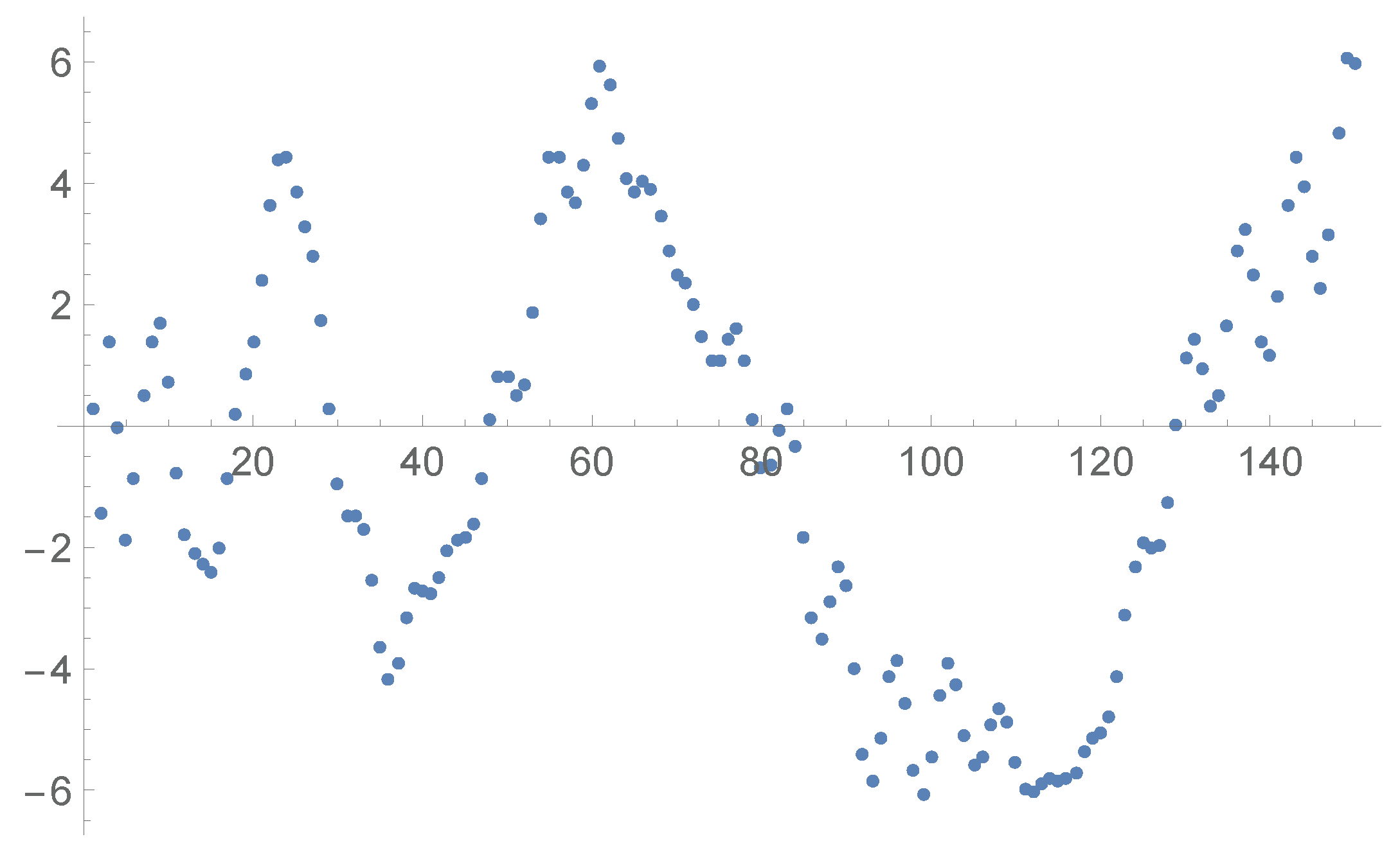
3.6. Some Charts

To clarify the logic of the decision-making inside the system we will provide the performance graphs describing pro-trend, long and short “trading” SPY and XAU (Gold & Silver) using the historical stock quotes once a day.

In the trading charts we provide, all signals, trades, positions, and returns can be seen under sufficiently high magnification. These charts are upon the optimization, i.e., not for the control periods, where the usage of “future” is excluded. We provide them mostly to clarify the “logic” of the system. Generally, using day-quotes only is a serious demerit; the system works reasonably, but the performance is significantly worse than trading SPY with three quotes a day.

Trading indices and commodities generally requires special approaches; see, e.g., (Fouque et al. 2003; Guasoni et al. 2019). Our system manages them reasonably, but it appeared necessary to increase the number of used categories to four, especially for SPY, versus our usual two to three for individual companies. Indices and some commodities are subject to many kinds of investing and hedging.

We use green, grey, and cyan correspondingly for the price-change, the returns based on level 1 signals, and those based on level 2 signals. Correspondingly, buy-sell signals are marked by blue-red rectangles-ovals; large ones mark trades for level 1 signals. See Figure 2 and Figure 3.

The moments of buy signals (all of them, of all levels) are marked by blue rectangles; the large ones correspond to level 1 signals. Accordingly, the sell signals are marked by red ovals; large for level 1. The blue and red vertical lines connect the level 1 execution points in the middle of the grey graph with those of the green equity chart. The returns graphs are changed only upon the terminations. The cyan graph is for the trades based on level 2 signals; here vertical lines are not used. The returns are in percent from the beginning of the graph.

To help the readers, we provide a fragment of the XAU in Figure 4. For example, here the first level 1 trade, marked by a large red oval (the first such), lasted till the first large blue rectangle and was executed at a loss: a vertical drop of the grey strip after the termination; XAU went up significantly and “unexpectedly” here. However, the next trade, which was short on the sell signal of level 2, shown by the next (small) red oval, appeared successful: a small increase of the cyan strip.

These two charts are upon the optimization, as well as in Figure 5, so they only evaluate the quality of the optimization, i.e., what our automated optimization procedure produced for this period. Only control periods (out-of-sample!) can be used to estimate real profitability. However, these charts clarify the “logic” of the system. Its unstable performance in the beginning is to be expected; the system needs sufficient “history”.

By simple returns here, we mean the total returns of SPY and XAU during the considered period (green curves). Only signals of levels 1,2 were used for “trading” (grey and cyan).

USING WEIGHTS. Let us provide the performance results for the following two periods: 3/21/2001/3/21 (9:30) –6/14/2001/6/14 (13:30), 2000/10/24 (9:30)–2001/6/10 (13:30), with correspondingly 60 and 113 days. The graphs below are in terms of “trading points”, when the system “visits the market” (receives quotes), here three times a day. So the number of points is approximately 180 and 339 for these control periods. We focus on using weights based on the prior optimization returns. Namely, the better optimization returns, the greater amounts to invest in this stock. Picking the companies with optimization returns greater than some limit is a variant of using such weights. The 75 companies were traded, long and short, pro-trend (i.e., essentially under mean reversion trading); they were mainly taken from the list of the most liquid ones. Sharpe Ratio (SR) is mean standard deviation.

By “straight”, we mean that the symbolic $100 were invested per any position (long or short) for the companies with the optimization (prior!) returns $>0\%$ and $>20\%$. The latter bound was adjusted to reduce the number of traded companies approximately by $50\%$. Generally, using the weights (or using “$>20\%$”) improves the performance, but not always significantly vs. “$>0\%$”, depending on the market types. “Red” is used for simple (actual) portfolio returns (based on the changes of share prices), “blue” for the returns the system achieves.

4. Pont, a Card Model

4.1. General Design

This game is a combination of bridge and Russian preference with poker-style auction. The name “bridge” was derived from earlier “biritch”, so we make it further from the origin (and shorter). It utilizes a standard deck of 52 cards or a smaller one of 36 cards. The auction is quite different from that of bridge and involves more risks. See here and below (Parlett 1991). The bidding does not use the denomination of suits. The player who starts the auction has no advantage. The cards may be updated while bidding, which resembles draw poker. The winner of the auction, the declarer, determines the final number of cards per hand as part of the declaration of the contract: the trump and the minimal number of tricks to be taken.

Following suit and the use of trump cards is similar to bridge-type games. The scoring is simpler than that of bridge. The declarer’s award is based on the value of the contract depending upon whether or not it was made. The game can be for 2, 3, 4 players, 2 partnerships, or for 1 versus computer. There is also a poker-like version. All variants are almost equally dynamic and playable.

Stock market connections. The game, especially the auction, can be considered a simple model of playing the market, especially under momentum “investing on news”. The bids then are some counterparts of the forecasts of share prices. The play checks the quality of the bid, but this is not related to real trading, where this quality is the return upon the termination of the position taken.

The number of cards per hand and the number of taken tricks reflect, respectively, the duration of the investment and the return. The downplay and misère resemble a bid selling short, but this is superficial. This is a game: just a model.

The suits are substitutes for the time-horizons of investments or the companies considered for investing. They are on equal grounds in pont in contrast to other bridge-type games. Given a suit, the better cards the more reasons to make it a trump. In our trading system, the category of the top bid determines the time-horizon of the investment, though the categories are ranked in contrast to suits in pont.

The players compete to become the declarer, which is somewhat similar to winning the “right” to invest. The upgrades and increases are designed to reflect real-time actions. The bids are actually 2-bids, which adds some “timing”; they depend on the size of hands (from 6 to 9), which has no counterparts in other bridge-type games.

The play itself has little to do with real playing the stock markets. For instance, the use of trump cards and positions of players around the table have no market analogs. The role of such special elements of card games is diminished in pont. However, they are inevitable; the game must be not too primitive. Also, more playable games have stronger roots in our psychology. Making pont playable was a challenge since it uses unusual fractional bids, related to our approach to risk-taking. This was a test of the principles of our trading system. we think that playing pont can help to get used to our 2-bids and in real playing the stock markets, possibly better than playing poker or bridge.

4.2. Description

The game uses a standard card deck of 52 cards for 4 players or a smaller, four-suit deck of 36 cards (from the ace down to the 6), when there are two or three players. In the case of 4 players, they may divide themselves into two partnerships; here the whole deck is used, too. The dealers are changed clockwise after each game. The cards are dealt singly in the clockwise order and face down, giving each player six cards. After the players pick up their hands, the dealer starts the auction by making the bid or passing.

Auction. A bid is a fraction N/D where the denominator D is from 6 to 8 and the numerator N is no larger than D. Generally speaking, the bid is the expected number of tricks to be taken (N) divided by the final number of cards per hand (D). The latter may be from 6 to 9. The fraction must be no smaller than 3/6 for 3 or 4 individual players, and no smaller than 4/6 for 2 players or partnerships. The fractions 4/8, 7/7, 8/8 are excluded. The bids 3/6, 4/7, and 5/8 are not allowed for 2 players, but are accepted for 3 or 4 players.

The auction proceeds clockwise with each player either making a bid that is not lower than the previous ones of other players; for instance, 4/6, 5/7, 6/8, 5/6, 6/7, 7/8, 6/6 may be claimed after 4/6. Otherwise, say “pass”. Bidding is forbidden after the first bid was made if a player has already passed. Passing is allowed after bidding only if there are other players who did not pass; also, the last remained (survived) player may not pass. The round of bidding continues until the last bid, when a player (who then becomes the closer) repeats his/her previous bid for the first time, or simply says “close”. If the others (two opponents for the team variant) passed after this, the closer becomes the declarer. Otherwise, there is no declarer.

More rounds are necessary if all players passed or at least two of them claim the same bid. To start the next round, the dealer upgrades the cards, giving out a card per hand face down. Then each player picks up the card and after this removes one card from the hand by laying it face down. i.e., the hands must be 6 again. Then the closer (or the dealer if all passed) claims first, repeating or enlarging his/her last bid, and the auction continues following the same rules until the first repetition. Those who passed during the previous rounds do not bid, unless all passed. The cards may be upgraded only twice.

Taking no tricks. If all passed after the last (the second) upgrade, the dealer leads to start the downplay notrump, where the players are trying to win the smallest number of tricks. The closer starts the downplay if two or more players (or both teams, if applicable) do not pass after the second upgrade, which is the last, but claim coinciding bids, i.e., neither of them is the winner.

At the end of the game, the number of taken tricks will be diminished by the minimum number, which is to make it zero at least for one player, and subtracted from the corresponding scores. In the case of 2 players, this diminished number must be divided by two before subtracting; e.g., the player who took 4 tricks will lose 1 point, which is 4 minus 2, the number of tricks of the opponent, divided by 2.

A player may claim misère, which means that no tricks will be taken. This may be done only before the first upgrade, and beaten by 6/7 or higher for 2 players (teams), by 5/6 or higher for 3 or 4 players. Misère is played no-trump. The declarer makes the opening lead by placing the card on the table face up. If there are 3 or 4 individual players all cards are placed face up on the table after this. It is the same for partnerships, but the partner does not participate laying his/her cards face down. The misère contract is defeated if either of the opponents finds the way where the declarer takes at least one trick.

The play. After the auction, the declarer may increase, asking the dealer to deal out 1 card per player face down. The procedure can be repeated several times, but the maximum number of cards per hand must be no greater than 9. The declarer picks up the cards every time. The others will do this only after the declaration of the contract. Then the declarer declares the contract, choosing the trump suit or no-trump, which is allowed, and stating the minimal number of tricks to be taken (including the partner’s tricks for the partnerships). The denominator “D” equals the number of cards per hand after the last increase.

The number of tricks to win cannot be smaller than the final number of cards per player (after the last increase) times the fraction from the last declarer’s bid. The bid “misère” can be changed by the declarer by the contracts 6/7, 7/8, 8/9, 6/6, 7/7, 8/8, 9/9. It is the same for 2, 3, 4 players, and the partnerships. Also, the last bid 6/8 can be changed by misère if there were no upgrades and increases. The partner’s hand is discarded face down when playing misère in the team variant.

The declarer starts the play trying to take enough tricks to fulfill the contract or take no tricks for misère. For partnerships, anytime during the play the declarer may ask the partner to place all his cards face up on the table and then he/she starts playing both of the partnership hands (unless in misère). All players have to follow suit if they can. Otherwise, they must trump. Only the declarer may lead a trump. Other players may do this only if they have no other suits left. The play lasts until the declarer (together with the partner if applicable) takes the necessary number of tricks or the contract is defeated.

Score system. At the end of the play, the declarer’s score goes up by the value of the contract, the number of tricks from the contract minus 3 for 2 players (or partnerships) and minus 2 for 3–4 individual players, if the contract was made. Otherwise, this value is subtracted from the score. If the last bid before the first upgrading was more or equal than 5/6, then this value goes up by one, called premium (when adding or subtracting). The same premium is added to misère, treated as 5/6 when calculating the score (3 points for 2 players/teams and 4 points for 3, 4 individual players). A fulfilled contract of fraction $=N/D=1$, gives 1 bonus point for 2 players (partnerships) and 2 bonus points for 3–4 individual players. For 3 or 4 individual players, successful contracts 5/6, 6/7, 7/8, 8/9, 9/10, and misère add 1 bonus point to the declarer’s score. In contrast to the premium, the bonus is not subtracted from the score if the contract fails.

There is another, somewhat more involved, variant of the pont score system with more “punishment” for defeated contracts. The play goes till the end. If the number of taken tricks is less than it was declared than the score of the declarer is diminished by the value of the contract multiplied by the number of missed tricks. Say, if the declare took the necessary tricks but one, the score becomes smaller by the value of the contract. This scoring system is for experienced players.

Finally, the rewards will be proportional to the scores of the players diminished by their arithmetic mean, that is the total of all scores divided by the number of players. The partners may redistribute the total partnership reward (the sum of their rewards). The standard recommended way is as follows. If both rewards are positive or negative then it is the same as for individuals. If the first reward is positive, the second is negative, and the total is negative, then the first partner does not pay. If the total is positive here, then the second partner receives nothing (and pays nothing).

Bidding table. The following table is the list of bids in increasing order and the corresponding minimum contracts for different numbers of cards per hand. The stars (adding 1 point each to the score) show the premium p for declaring during the first round of the auction and the bonus b for making the contract.

3–4 individual players		contracts	2 players(partnerships)
names	b p bids:	tricks/cards	:bids p b	names
1	3/6:	3/6, 4/7, 4/8, 5/9	: —	—
1+1	4/7:	4/6, 4/7, 5/8, 6/9	: —	—
1+2	5/8:	4/6, 5/7, 5/8, 6/9	: —	—
2	4/6:	4/6, 5/7, 6/8, 6/9	:4/6	1
2+1	5/7:	5/6, 5/7, 6/8, 7/9	:5/7	1+1
2+2	6/8:	5/6, 6/7, 6/8, 7/9	:6/8	1+2
m	* * m/6:	...., 6/7, 7/8, 8/9	:5/6 *	2
3	* * 5/6:	...., 6/7, 7/8, 8/9	:m/6 *	m
3+1	* * 6/7:	6/6, 6/7, 7/8, 8/9	:6/7 *	2+1
3+2	* * 7/8:	6/6, 7/7, 7/8, 8/9	:7/8 *	2+2
4	** * 6/6:	6/6, 7/7, 8/8, 9/9	:6/6 * *	3.

Here misère (m = m/6) has the same list of admissible contracts as 5/6 but is ranked higher for 2 players (partnerships) and lower for 3 or 4 individuals. Recall that the misère contract may be played after the last bid 6/8 or smaller; m/6 is omitted in the column of contracts.

The names of the bids are convenient when bidding. The name gives the number of additional cards (after +) and the value of the (lowest) contract coinciding with the bid, calculated without the premium and bonus. For instance, the value of 2 + 2 = 6/8 for 3, 4 players equals 2 + 2 = 4. For 2 players, the contract 1 + 2 = 6/8 gives 3 points.

4.3. Variants

Basic-Pont (BP). The simplest version of the game is the basic pont, which is played without misère, and “premium”. The table is also simplified by dropping the bids of denominator 8 (the +2-bids):

3–4 individuals		contracts	2 players(teams)
names	b bids:	tricks/cards	:bids b	names
1	3/6:	3/6, 4/7, 4/8, 5/9	: —	—
1+1	4/7:	4/6, 4/7, 5/8, 6/9	: —	—
2	4/6:	4/6, 5/7, 6/8, 6/9	:4/6	1
2+1	5/7:	5/6, 5/7, 6/8, 7/9	:5/7	1+1
3	* 5/6:	5/6, 6/7, 7/8, 8/9	:5/6	2
3+1	* 6/7:	6/6, 6/7, 7/8, 8/9	:6/7	2+1
4	** 6/6:	6/6, 7/7, 8/8, 9/9	:6/6 *	3.

Poker-Pont (PP). Another variant is poker pont for 2, 3, 4 individual players. It follows the table of the basic pont, without bonuses.

bids:	contracts	5/7:	5/6, 5/7, 6/8, 7/9
3/6:	3/6, 4/7, 4/8, 5/9	5/6:	5/6, 6/7, 7/8, 8/9
4/7:	4/6, 4/7, 5/8, 6/9	6/7:	6/6, 6/7, 7/8, 8/9
4/6:	4/6, 5/7, 6/8, 6/9	6/6:	6/6, 7/7, 8/8, 9/9.

PP-betting. As in poker, each player puts up ante (one chip or more) to form a pool, which consists of the pot and the sectors, one for a player. A player always puts chips in the corresponding sector. The dealer starts betting, adding chips to the pool or putting nothing, passing. The player on the dealer’s left may pass, call by putting the same, or raise by adding extra chips of his/her own. Other players continue clockwise until all have finally called any raises. A player may raise after passing if the latter was before the first raise. Passing is allowed after raising or calling if there are other players who did not pass.

The first player who calls without adding is the closer. If all other players passed, the closer is the declarer. If there is no declarer, the dealer upgrades cards and the closer starts another round of betting by raising or doing nothing. Those who passed before, if at least one player raised, may not bid. There are optional upgrades in poker pont; they may be omitted. Then the card will be dealt to the next player. A player who upgrades puts a chip to his/her sector (per each new card). The number of upgrades is no more than three (for four rounds of betting). If still all pass after the last upgrade then the ante goes to the pot, the dealer is changed clockwise, and a new game starts.

PP-play. If there are two or more players who put the same number of chips (regardless of the extra chips for upgrades which may be different), then the closer begins one round of bidding among those players only. It is as in the basic pont; the declarer is a player claiming the highest bid. If still there is no declarer, there will be no more upgrades. Then the dealer moves all chips but ante from the sectors to the pot, and the next dealer starts a new game.

The declarer may increase several times (no more than three), adding a chip per increase to the pool. After the declaration of the contract, all opponents pick the cards and respond or pass clockwise starting with the first on the declarer’s left. One must add one chip per each increase (totally, the current number of cards per hand minus 6) to the pool to respond and become an active opponent. Other opponents are passive. However, all participate in the play, which follows the standard rules.

The declarer leads and wins the pool (including the pot) when making the contract. If the latter is defeated then all the opponents, active and passive, take chips back from their sectors and the active opponents divide the declarer’s chips and the pot among themselves proportionally to the number of taken tricks. The fractions are ignored and the remaining chips (if any) go to the pot. If there are no active opponents, the declarer takes his/her chips back even in the case of the failure (but not the pot). The contract has to be the minimal possible for the current number of cards per hand. Namely, 3/6, 4/7 for 3–4 players, 4/6, 5/7 for 2 players, and 6/8, 6/9 for either. It may not be lower than the last bid if there has been a round of bidding to determine the declarer.

4.4. Comments

Additional rules. Extra penalties can be added for breaking the rules. The opponents may decide to diminish the declarer’s or partnership’s score by the value of the contract if the declarer (partnership) made a mistake against the rules when playing. Vise versa, in the case of an opponent’s mistake, the declarer has the right to consider the contract to be fulfilled and the other player(s) may decide to subtract its value (or its doubled value) from the score of the opponent whose fault is it. In poker pont, the contract is considered to be defeated in the case of a declarer’s mistake. If it is an opponent’s mistake, the chips from the pool are distributed as if the contract were defeated, and the opponent who made a mistake gives this very number of chips to the declarer. These are basics, to be developed by players.

The following regulation could improve the coordination of the opponents (for 3 or 4 individual players) and may be added to the rules. The opponents have to play the lowest card higher than the card of the declarer& partner to win the trick if they can. However, the card must be the lowest possible to leave the trick to an opponent whose card already beats the cards of the declarer and partner. As to the partnerships, a general regulation is to at least repeat the bid of your partner if you have two sure tricks or more, i.e., could win two tricks for any trump. For instance, it may be either “A A”, or “A K” in the same suit, or “A” in one suit and “K Q” in another. When you pass, but the opponents don’t, it can stimulate your partner to pass or claim misère. To avoid this, it makes sense to bid if you can count on three (or more) tricks upon declaring your trump, especially if you have honors and the hand seems good for the increases. Just to give an example of such coordination.

A computer version. The computer realization of the variant for two players is based on the following principles. The computer is programmed to select the best one considering several random choices of the hand of the player (taking into account all information about the cards of the player appearing during the play). It does the same when bidding and declaring, but diminishes the most likely bid and contract by one level. The simplest one-way version is when the computer never bids (and has no score), and the player either determines the contract (without upgrades) and then plays following the standard rules or passes subtracting 2 points from his/her score. It follows basic pont. However, the bidding scale and the admissible contracts start from 4/7 considered as 0 + 1 and giving 1 point. More generally, 0 + k, which means (3 + k)/(6 + k), is counted as k points for k = 1, ..., 6.

The computer basic strategy is to win the trick led by the player with the smallest possible card and to play the lowest card otherwise. If it has no proper suit and no trump left, the card can be the lowest (from the shortest suit, if there are several cards of the same rank). However, the suits where the player has no cards according to the information during the process of play are considered the best. When the computer leads, then the suit where the player has no cards is the first choice too. If the highest card (one of them if there are several of the same rank) has the adjacent one in the same suit (say, the pairs “A K” or “K Q” are adjacent), or the next card in the suit is lower by 4 or more (say, “A 10”), then this is the second choice for leading. Otherwise, the suit must be the longest and the card the highest among the longest suits. However, the longest suit where the two highest cards are adjacent is considered first. If still there are several choices the computer decides randomly. These are, of course, very basic considerations; the actual computer program can be significantly more developed.

5. Main Findings and Steps

As almost always with econophysics and modeling economic processes based on physics principles, including investing and trading, the motivation for the usage of ODE, PDE, SDE is of great importance. The justification of our approach to modeling momentum processes in stock markets is based on behavioral finance and cognitive science. This is not something unexpected. Let us outline the main steps of our analysis.

5.1. MRT and Two-Bids

The first step is the marshmallow test, a demonstration of the usage of different time scales. Even in such a “baby example”, it is clear that the power-type growth of price-functions with exponents $<1$ can be expected. The second step is our analysis of thinking fast due to Kahneman. We argue that the following is of key importance for modeling “momentum trading” (mostly short-term): investors must decide quickly and almost always on the basis of incomplete information.

Kahneman’s approach is qualitative and too basic, which is insufficient for us. Therefore the third step is to make it quantitative: we propose the concept of MRT, momentum risk taking. The fourth step is to justify the usage of 2-bids, which are in terms of the expected returns during the variable time-intervals.

This definitely requires clarification. Generally, bids are “one-dimensional”. The contract-type card games, which reflect many of the auction principles people use, are in different suits, but they are 1-bids. Replacing cards in draw poker is some kind of adding time to the bids (a similar kind of uncertainty), but this is not a contract game. We designed pont, a poker-type card game with bridge-type auction and contracts, to demonstrate that 2-bids, with variable sizes of the hands, can be quite “playable”.

Pont provides some reasonable expectations for the number of categories, which are investing horizons for us. There are four suits in cards. For us, this becomes seven horizons: hours, days, weeks, months and three intermediate ones. The suits are ranked lexicographically in card games. The ranking of our categories is much more meaningful. To give an example, the first bid in category 1, which is $1\%$ per 1 h, provides $3\%$ in 1 day according to the g-formula, which is greater than the first bid in category 3, which is $2\%$ per day. So if these bids arrive simultaneously, then the former bid “wins”, in category 1.

Practically, from two to four categories were used for trading individual equities and reasonably uniform portfolios; though up to five can be suitable for trading the spider and indices. The optimization is performed in two ways: for individual equities and for the whole portfolio. It is not always true that the former way is more profitable.

5.2. ODE and Sample Curves

Assuming the MRT concept, obtaining the differential equations is relatively straightforward. The key output is that the growth of price-functions is power-type: $\sim t^r$ in terms of time t. Here $r\approx 1/2$ for positions lasted weeks and longer, but can become $r\approx 0.137$ short-term, say for day-trading. This is one of the key discretization assumptions in this paper and for our trading system.

Generally, sampling of this sort is frequently used in machine learning. For instance, Navier–Stokes equations can be solved this way: by finding the closest “sample solutions”, when the list of basic solutions is produced in advance.

The table of our basic price-functions is presented in (23)–(26). It is the result of our analysis of the charts of different equities and portfolios for various time scales. The corresponding 2-bids are linearly ordered; the ones in different categories can be compared, not only those in the same category (for the same investment horizons). This table proved to work well for many portfolios. Such 2-bids can be useful beyond the stock markets, but we checked its efficiency only for trading market instruments.

Obviously, different tables lead to different trading systems, which can be profitable as well. However, such tables must satisfy sharp restrictions. There must be inequalities between the corresponding returns for different categories if the expected durations of positions overlap: the smaller the number of the category the greater the return, as in the example considered above.

There are also discretization matters. The basic returns must be ideally integers, to be used manually, though this is not that important for automated trading. Also, given a category, the number of considered durations of the bids must be not large. The bids are discrete by their nature; the minimal return for a given category (for the time-unit of the corresponding investment horizon) must satisfy some minimum requirement, which is a clear counterpart of “action potentials” in neuron systems.

Next, not all bids become trading signals. A bid must reach some threshold in its category. If this holds, then the auction begins: there can be signals from several categories. The “winner” of the auction is determined using the table.

The auctions are performed regardless of the existing positions. If there is already a position in the same direction for the instrument under consideration, then an additional position will be open. We call such signals/positions of level 2; the levels can be greater than 2. If there is no current position for this instrument or it exists in the opposite direction, then this position (if any) will be terminated and the new one will be created with the expected duration and return according to the bid.

5.3. From Signals to Trades

Assuming that the winning bid became a signal and that this signal resulted in opening the corresponding positions, the termination curve will be started corresponding to this bid. It gives the future expected returns for some period depending on the category of the bid. They can be actually used for forecasting.

Such curves are “plotted” somewhat below the actual returns near the moments when the trade begins. This is controlled by an important parameter of the system (subject to the optimization). When the real return becomes below the termination curve (considered in the same category and subject to proper discretization), then the position will be terminated. This is essentially the algorithm we employ. However, some additional factors are considered.

There are some thresholds for the difference counterparts of the derivatives of price-functions that are required to be satisfied to start or to terminate positions. The change of the price must be large enough to trigger a trading action. The usage of derivatives and their difference counterparts is standard in almost any trading systems, but they are very volatile and generally insufficient to be used as main trading signals. Adding this feature to our system appeared necessary to increase its profitability, to provide faster responses to the changes of share prices, and to prevent “hangs” with some positions. The system is fully automated and the hangs are not allowed to be corrected manually.

The categories, the minimal bids, the positions of the termination curves below the actual ones, and the thresholds for the difference counterparts of derivatives are subject to the optimization. The system was designed to work for months in a completely autonomous regime, including auto-optimization of the parameters (normally during weekends) and it worked as such.

Mostly, we used from two to four categories, which depends on the type of the instrument and the average durations of investments requested by the end users of our trading system. The other parameters are subject to constant optimization.

5.4. Other Aspects

Trading systems, especially fully automated ones, involve many procedures and algorithms (very many in our case). Let us say little something about our optimization procedures. Due to a limited number of parameters, we mostly use the gradient method, which works very well. It is very rare when significant returns and good Sharpe ratios cannot be achieved with individual equities and reasonably homogeneous portfolios. The programs we use “capture” such jumps in the performance (for some combinations of parameters), which occur almost always, but are generally not unique.

There are many practical matters to manage. For instance, our system constantly produces full backups and allows emergency restarting. Splits, the share price adjustments due to the dividends, renaming the stocks are automatically performed every day. Even proper encoding the stocks regardless of their current symbols is quite a challenge: they occur very many times in various programs in our system.

Producing trading signals is the key output of our and any system, followed by their execution by the end users. Constant monitoring of the performance of the portfolios is a necessity, too, including collecting, processing, and reporting the results. All kinds of statistical data were produced at the end of every trading day.

We managed many portfolios (in the research mode and real-time), and, importantly, multiple lines trading the same portfolio (for different categories and different sets of optimization parameters). This provided the necessary diversification, which worked reasonably even for individual stocks and relatively small portfolios.

An interesting way for creating a new line was by shifting the existing one by 1–2 h. Then such a pair of lines worked similarly for some time, but eventually, their trades became quite different (even with coinciding parameters). The profitability of such “parallel” lines was generally comparable (but not always). Changing the trading modes was another possibility for producing multiply lines. For instance, the lines could be with or without short trading, though almost always both modes were present.

We note that the system was mostly used under hedging; it was provided by the end users, but it can do this itself. Generally, strict hedging can create problems with the performance: it is not always “momentum”. However, the system can be used this way.

Complete information for each and every bid and signal is stored by the system. The number of signals and trades is huge, but checking “manually” the logic of some of them was of importance (at least for designing new lines). This was generally possible because our parameters are all meaningful: categories, various “action potentials”, etc. Practically, the convenient charts presenting trading signals and the corresponding trades were mostly used practically to control the “logic” and the “health” of trades. This means the system is “trustworthy” in this respect, not a “black box”.

6. Concluding Remarks

6.1. The Key: Bidding Tables

Let us stress that our trading system is not a black box; the logic of its decisions concerning trading stocks (any instruments) can be fully reconstructed and understood; cf. (Horel and Giesecke 2019). We found not many situations where its decisions could be questioned on the basis of the usual technical analysis, though the system uses the stock-charts and its own prior decisions in novel ways. Pont clarifies some principles of our approach and tests them “psychologically”. We also hope that playing pont can help to get used to our 2-bids.

The bidding table of pont and the one used for the system’s 2-bids $(b,c)$ are similar, and this is not just an analogy! The auction and bidding seem fundamental for any intelligence. This can be within some expert system, inside our brain, or AI. Poker and contract card games serve humankind well as a risk-taking playground: they obviously capture something important about human cognition. See (Parlett 1991).

Obviously, using computers makes bidding formal and not “immediately understandable”. The automated optimization and deep learning are even more difficult to interpret, even if every optimization step can be seen in detail, as in our programs. Generally, machine learning is fully “trustworthy”, only if the results can be clearly interpreted “humanly”. In our trading system, the optimization is mostly of this kind due to the small number of parameters our system deals with. The main parameters are the categories, the modes (long/short, pro/counter), key thresholds, and some derived parameters like the average duration of positions; all are meaningful to investors. Our usage of power functions in the tables of 2-bids has solid grounds too, as we tried to demonstrate.

The discretization, which is necessary to separate noise from signals, is not really “intuitive”, but the “action potentials” are always necessary and any usage of computers requires discretization. In our trading system, we made the discretization as “human” as possible. The author of the paper is a specialist in discrete theories (mostly “integrable”), but the market reality resulted in non-standard auction-style stratified discretization. It is new, though using the data stratification and sample curves is common in neural networking. It is likely that our approach reflects the risk-taking processes in our brain; its successful market implementation can be regarded as some confirmation.

The importance of finding optimal relations between the decisions and sampling frequencies is well recognized. Let us quote (Singleton 2006):

Though available data are sampled at discrete intervals of time—daily, weekly, and so on—it need not be the case that economic agents make their decisions at the same sampling frequency. Yet it is not uncommon for the available data, including their sampling frequency, to dictate a modeler’s assumption about the decision interval of the economic agents in the model. Almost exclusively, two cases are considered: discrete-time models typically match the sampling and decision intervals—monthly sampled data mean monthly decision intervals, and so on—whereas continuous-time models assume that agents make decisions continuously in time and then implications are derived for discretely sampled data. There is often no sound economic justification for either the coincidence of timing in discrete-time models, or the convenience of continuous decision making in continuous-time models.

This is actually the key problem we address in our trading system and this paper: how to coordinate different “decision intervals” and what is optimal decision-making based on a simultaneous analysis of several “frequencies”. This is a must for AI systems focused on trading and of obvious importance well beyond stock markets.

Timing the market is and always was a great challenge, but now we have a new chapter: a systematic AI-based research and optimization of the process of investing. The usage of AI is a must here because the only reliable way to test the performance of any trading system is (a) when it is fully(!) automated (machine learning included), (b) when someone else (not the creator) runs it, (c) the design and analysis of the experiments is as rigorous as possible, and (d) all findings are confirmed by real-time trading, which obviously requires full automatization.

We provide a sufficiently complete description of the basic principles of our trading system and the ways it was tested. Not all aspects of our approach were addressed here. The system consists of a lot of programs; many are used for technical processing data, including but not limited to managing historic and real-time quotes, practical matters like splits-dividends, and so on. Quite a few serve the optimization, historical and real-time. The real-time optimization uses the system’s own history of trades, upgrading the parameters “while trading” (normally during weekends). Historic simulations require a lot of special software, too. This is on top of actual trading programs and those monitoring the performance. The coordination of such a ramified combination of service, optimization, and action programs is quite a test for any system; this is no different from the ways our brains work.

6.2. Beyond Stock Markets

The stock markets can be considered a great model for many aspects of decision-making. In our approach, the impact of “events” is measured indirectly, via the responses of the “agents”, which is quite standard in sociology and statistical physics. Many of our findings seem of a universal nature. For instance, our equations connecting price-functions with the news-functions can be equally used to model the relation between the expected resources for a task and those actually used, presumably including our brain.

“Investing” has its special features. Under momentum risk-taking, the agents seek to optimize their actions: (a) entering the “game” quickly when a clear signal is detected, and (b) exiting when some price-function reaches expected levels. Practically, we use here tables of 2-bids and forecasting-termination curves. Theoretically, power functions and their generalizations, Bessel and hypergeometric functions, are of significance here, as it was demonstrated in Section 2.

Importantly, we focus on the time-intervals when the news impact remains growing. The main reason is obvious: an objective of any trading is to capture local maxima of price-functions. It is quite likely that other events will occur before the impact of particular news reaches some saturation or periodicity due to profit-taking; they will certainly interfere. Practically, only short-term news impacts and relatively short-term forecasts makes sense for momentum trading.

This can be generally applicable to MRT in our brain, though with a huge number of neurons and very complex interactions. Assuming this, “events” reveal themselves via some waves of “mass behavior”. Accordingly, such waves are likely to be the main information available to individual neurons and the key source of their “decisions”, governed by action potentials and similar mechanisms. Eventually, our brain creates some “images” of the underlying events. This way, we are even able to form abstract concepts, such as space-time. Philosophically, let us at least mention here, Kant; see, e.g., (Janiak 2016).

Our analysis of stock markets, especially the simplicity of the basic differential equations we propose, can be an indication that the power-laws for the impacts of “events”, auction-type procedures, and certain price-functions are present in the biology of the brain at the neural level. This is related to neural networking. The price-function generally measures the current importance of the event and the corresponding expected resources needed for its analysis. Our brain will try to diminish the neural activity when some “price-levels” are reached, though the price (the importance) varies depending on the intensity of the triggered brain activity. This can even result in periodic “waves of interest” in an event: an auto-mechanism for its abiding analysis, which we mathematically associate with Bessel functions. There is a lot of “macro-management” here, beyond MRT, say corrections of the failed decisions. The mechanisms of such conscious or unconscious “re-visiting” the analysis of past events are obviously complicated.

Let us mention here that the systems of differential equations and their solutions, Bessel-type and in terms of elementary functions, proved to be very useful for modeling epidemics. They describe the curves of total detected infections for COVID-19 in many countries almost with the accuracy of physics laws.

6.3. MRT: Main Findings

(1)

Cognitive science. The origin of our approach in cognitive science is the concept of momentum risk-taking, MRT, which can be defined as short-term decision-making and forecasting based on the real-time monitoring of the actions of other agents. Poker and our pont are good examples of games with similar data, but stock markets are of course the main source of this concept. In contrast to thinking-fast and thinking-slow from (Kahneman 2011), when the “agents” can generally choose between two modes of thinking (unless in specially crafted experiments), there is no such choice here and high uncertainty is generally involved. Investors are assumed to decide “optimally” on the basis of the current news impact. Our restriction to short-term decisions and forecasts makes it possible to propose a mathematical, quantitative model of MRT, in contrast to thinking-fast, which is generally qualitative.

(2)

Toward general-purpose AI. The restriction to MRT seems a realistic approach to general purpose AI systems. MRT is obviously one of the key parts of any intelligence, not only with humans. There is an astonishing universality of momentum risk-taking; those who master it in one field, can generally use their expertise in other fields upon proper (sometimes little) training. We think that almost the same risk-taking curves (we call them forecasting or termination curves) govern quite a spectrum of short-term risk-management tasks and that the corresponding “learning” is quite uniform almost regardless of the concrete tasks. The neural action potentials provide some discretization and timing, but there must be other mechanisms in the biology of the brain serving MRT. Some mechanisms are well beyond MRT, for instance, the analysis of prior decisions. Expecting errors and correcting them is what intelligence is about.

(3)

Modeling MRT. Importantly, MRT can be modeled mathematically, which we perform thanks to our focus on short-term management. The power growth of our forecasting curves holds only for relatively short periods “after the event”. The corresponding differential equations modeling news impact seem sufficiently reliable to us. The trading system described in Section 3 is an experimental confirmation: it is based on the “power-law” for price-functions with exponents depending on the corresponding investment horizons. Mathematically, an argument in favor of our approach is a model of profit-taking in terms of Bessel functions. This relates the periodicity of profit-taking to the asymptotic periodicity of Bessel functions: a new approach to the market volatility, one of the key subjects in quantitative finance.

(4)

Market volatility. The closest approach to ours that we found in the vast literature on volatility in stock markets is based on the fractional Brownian motion, fBM with Hurst exponents reflecting the investment horizons. For instance, the usage of fBM explains theoretically why the volatility is extreme for day-trading (with low Hurst exponents). Some statistical variant of our approach is a consideration of a linear combination of 2-3 fBM corresponding to “heterogeneous time scales”. Let us refer here at least to (Cheridito 2001; Delpini and Bormetti 2015); see Section 2 above. The approach via fBM does not separate the profit-taking from the “stochastic” volatility of stock markets, which is of key importance for practical trading (and our system). Our theoretical analysis indicates that Bessel processes, generalizing fBM, are likely to emerge here.

(5)

Some perspectives. As was quoted in the Introduction, we are decades away from general purpose AI (USA National Science & Technology Council). However, one can hope that some “prototypes”, can be designed faster than this. Even limited “deep learning” we (mostly) use in our experiments described in Section 3, provided efficient “human-like” behavior of our trading system. It was entirely focused on investing, but designing this kind of MRT for various tasks (with uniform and sufficiently fast machine learning) seems quite doable. It will require (i) further developing the mathematical model of MRT we suggested, (ii) finding its roots in the biology of the brain and psychology, (iii) improving the learning and risk-taking algorithms and making them really universal, (iv) experiments, and more experiments.

References

1. Abramowitz, Milton, and Irene A. Stegun, eds. 1972. Handbook of Mathematical Functions with Formulas, Graphs, and Mathematical Tables. National Bureau of Standards, Applied Mathematics Series 55, Tenth Printing with Corrections; Cambridge: Cambridge University Press. [Google Scholar]
2. Almgren, Robert. 2012. Optimal Trading with Stochastic Liquidity and Volatility. SIAM Journal on Financial Mathematics 3: 163–81. [Google Scholar] [CrossRef]
3. Andersen, Torben G., Gökhan Cebiroglu, and Nikolaus Hautsch. 2017. Volatility, Information Feedback and Market Microstructure Noise: A Tale of Two Regimes. Rochester: SSRN. [Google Scholar]
4. Andersen, Torben G., Tim Bollerslev, and Steve Lange. 1999. Forecasting financial market volatility: Sample frequency vis-a-vis forecast horizon. Journal of Empirical Finance 6: 457–77. [Google Scholar] [CrossRef]
5. Bank, Peter, H. Mete Soner, and Moritz Voß. 2017. Hedging with temporary price impact. Mathematics and Financial Economics 11: 215–239. [Google Scholar] [CrossRef] [Green Version]
6. Borodin, Alexei, and Ivan Corwin. 2014. Macdonald processes. Probability Theory and Related Fields 158: 225–400. [Google Scholar] [CrossRef] [Green Version]
7. Borovykh, Anastasia, Sander Bohte, and Cornelis W. Oosterlee. 2019. Dilated convolutional neural networks for time series forecasting. Journal of Computational Finance 22: 73–101. [Google Scholar] [CrossRef] [Green Version]
8. Bouchard, Bruno, Gregoire Loeper, H. Mete Soner, and Chao Zhou. 2018. Second order stochastic target problems with generalized market impact. arXiv arXiv:1806.08533v1. [Google Scholar] [CrossRef] [Green Version]
9. Bouchaud, Jean-Philippe. 2001. Power laws in economics and finance: Some ideas from physics. Quantitative Finance 1: 105–12. [Google Scholar] [CrossRef]
10. Broadie, Mark, Yiping Du, and Ciamac Moallemi. 2011. Efficient risk estimation via nested sequential simulation. Management Science 57: 1172–94. [Google Scholar] [CrossRef] [Green Version]
11. Brogaard, Jonathan, Terrence Hendershott, and Ryan Riordan. 2014. High-Frequency Trading and Price Discovery. The Review of Financial Studies 27: 2267–306. [Google Scholar] [CrossRef] [Green Version]
12. Buchanan, Bonnie. 2019. Artificial Intelligence in Finance. London: Alan Turing Institute. [Google Scholar] [CrossRef]
13. Cartea, Alvaro, Sebastian Jaimungal, and Jose Penalva. 2015. Algorithmic and High-Frequency Trading. Cambridge: Cambridge University Press. [Google Scholar]
14. Chan, Patrick, and Ronnie Sircar. 2015. Optimal Trading with Predictable Return and Stochastic Volatility. Rochester: SSRN. [Google Scholar]
15. Cherednik, Ivan. 2005. Double Affine Hecke Algebras. LMS Lecture Note Series, 319; Cambridge: Cambridge University Press, 446p. [Google Scholar]
16. Cherednik, Ivan. 2018. Affine Hecke Algebras via DAHA. Arnold MJ 4: 69–85. [Google Scholar] [CrossRef] [Green Version]
17. Cherednik, Ivan. 2020. Momentum managing epidemic spread and Bessel functions. Chaos, Solitons & Fractals 139: 110234. [Google Scholar] [CrossRef]
18. Cherednik, Ivan. 2021. Modeling the waves of COVID-19. medRxiv. [Google Scholar] [CrossRef]
19. Cherednik, Ivan, and Xiaoguang Ma. 2013. Spherical and Whittaker functions via DAHA II. Selecta Mathematica (N.S.) 19: 819–64. [Google Scholar] [CrossRef]
20. Cheridito, Patrick. 2001. Mixed fractional Brownian motion. Bernoulli 7: 913–34. [Google Scholar] [CrossRef]
21. Cheridito, Patrick, and Tardu Sepin. 2014. Optimal trade execution under stochastic volatility and liquidity. Applied Mathematical Finance 21: 342–62. [Google Scholar] [CrossRef]
22. Chinthalapati, V. L. R., and Edward Tsang, eds. 2019. Special issue on algorithms in computational finance. Algorithms 12: 4. [Google Scholar]
23. Conrad, Jennifer, and Gautam Kaul. 1998. An anatomy of trading strategies. The Review of Financial Studies 11: 489–519. [Google Scholar] [CrossRef]
24. Delpini, Danilo, and Giacomo Bormetti. 2015. Stochastic volatility with heterogeneous time scales. Quantitative Finance 15: 1597–608. [Google Scholar] [CrossRef] [Green Version]
25. Engle, Robert F., and Robert Ferstenberg. 2007. Execution risk: It is the same as investment risk. Journal of Trading 2: 10–20. [Google Scholar] [CrossRef]
26. Engle, Robert F., and Victor. K. Ng. 1993. Measuring and testing the impact of news on volatility. Journal of Finance 48: 1749–78. [Google Scholar] [CrossRef]
27. Fouque, Jean-Pierre, and Joseph A. Langsam, eds. 2013. Handbook on Systemic Risk. Cambridge: Cambridge University Press. [Google Scholar]
28. Fouque, Jean-Pierre, George Papanicolaou, Ronnie Sircar, and Knut Solna. 2003. Short time-scales in S&P 500 volatility. Journal of Computational Finance 6: 1–23. [Google Scholar]
29. Gabaix, Xavier. 2016. Power laws in economics: An introduction. Journal of Economic Perspectives 30: 185–206. [Google Scholar] [CrossRef] [Green Version]
30. Gatheral, Jim, Thibault Jaisson, and Mathieu Rosenbaum. 2018. Volatility is rough. Quantitative Finance 18: 933–49. [Google Scholar] [CrossRef]
31. Glosten, Lawrence, and Paul Milgrom. 1985. Bid, ask and transaction prices in a specialist market with heterogeneously informed trader. Journal of Financial Economics 14: 71–100. [Google Scholar] [CrossRef] [Green Version]
32. Gökay, Selim, Alexandre F. Roch, and H. Mete Soner. 2011. Liquidity models in continuous and discrete time. In Advanced Mathematical Methods for Finance. Edited by Di Nunno Giulia and Øksendal Bernt. Heidelberg: Springer, pp. 333–366. [Google Scholar]
33. Guasoni, Paolo, Antonella Tolomeo, and Gu Wang. 2019. Should commodity investors follow commodities’ prices? SIAM Journal on Financial Mathematics 10: 466–90. [Google Scholar] [CrossRef]
34. Guasoni, Paolo, Zsolt Nika, and Miklòs Ràsonyi. 2017. Trading fractional Brownian motion. SSRN Electronic Journal 10: 769–89. [Google Scholar] [CrossRef]
35. Gubiec, Tomasz, Tomasz Werner, Ryszard Kutner, and Didier Sornette. 2012. Modeling of super-extreme events: An application to the hierarchical Weierstrass-Mandelbrot Continuous-time Random Walk. The European Physical Journal Special Topics 205: 27–52. [Google Scholar]
36. Gu&#xE9;ant, Olivier. 2013. Permanent market impact can be nonlinear. arXiv arXiv:1305.0413v4. [Google Scholar]
37. Guéant, Olivier, Jean-Michel Lasry, and Pierre-Louis Lions. 2011. Mean field games and applications. In Paris-Princeton Lectures on Mathematical Finance 2010. Lecture Notes in Mathematics 2003. Berlin and Heidelberg: Springer, pp. 205–66. [Google Scholar]
38. Ho, Jonathan, and Stefano Ermon. 2016. Generative Adversarial Imitation Learning. Advances in Neural Information Processing Systems 29: 4565–73. [Google Scholar]
39. Horel, Enguerrand, and Kay Giesecke. 2019. Towards explainable AI: Significance tests for neural networks. arXiv arXiv:1902.06021v1. [Google Scholar] [CrossRef]
40. Janiak, Adrew. 2016. Kant’s Views on Space and Time. In Stanford Encyclopedia of Philosophy, Winter 2016 Edition. Edited by E. Zalta. Available online: https://plato.stanford.edu/archives/win2016/entries/kant-spacetime/ (accessed on 1 October 2021).
41. Kahneman, Daniel. 2011. Thinking, Fast and Slow. New York: Farrar, Straus and Giroux. [Google Scholar]
42. Katori, Makoto. 2011. Bessel process, Schramm-Loewner evolution, and Dyson model. arXiv arXiv:1103.4728v1. [Google Scholar]
43. Korajczyk, Robert A., and Ronnie Sadka. 2004. Are momentum profits robust to trading costs? Journal of Finance 59: 1039–82. [Google Scholar] [CrossRef]
44. Mantegna, Rosario N., and H. Eugene Stanley. 2000. Introduction to Econophysics: Correlations and Complexity in Finance. Cambridge: Cambridge University Press. [Google Scholar]
45. Moazeni, Somayeh, Thomas F. Coleman, and Yuying Li. 2010. Optimal portfolio execution strategies and sensitivity to price impact parameters. SIAM Journal Optimization 30: 1620–54. [Google Scholar] [CrossRef] [Green Version]
46. Novak, Andrej, Daniel Bennett, and Tomas Kliestik. 2021. Product Decision-Making Information Systems, Real-Time Sensor Networks, and Artificial Intelligence-driven Big Data Analytics in Sustainable Industry 4.0. Economics, Management, and Financial Markets 16: 62–72. [Google Scholar]
47. O’Hara, Maureen. 2015. High frequency market microstructure. Journal of Financial Economics 116: 257–70. [Google Scholar] [CrossRef]
48. Opdam, Eric M. 1993. Dunkl operators, Bessel functions and the discriminant of a finite Coxeter group. Compositio Mathematica 85: 333–73. [Google Scholar]
49. Parlett, David. 1991. A History of Card Games. Oxford: Oxford University Press. [Google Scholar]
50. Singleton, Kenneth J. 2006. Empirical Dynamic Asset Pricing: Model Specification and Econometric Assessment. Princeton: Princeton University Press. [Google Scholar]
51. Sirignano, Justin, and Rama Cont. 2019. Universal features of price formation in financial markets: Perspectives from deep learning. Quantitative Finance 19: 1449–59. [Google Scholar] [CrossRef]
52. Watson, George Neville. 1944. A Treatise on the Theory of Bessel Functions, 2nd ed. Cambridge: Cambridge University Press. [Google Scholar]
53. Watts, Tyler W., Greg J. Duncan, and Haonan Quan. 2018. Revisiting the marshmallow test: A conceptual replication investigating links between early delay of gratification and later outcomes. Psychological Science 29: 1159–77. [Google Scholar] [CrossRef]
54. Yang, Xuebing, and Huilan Zhang. 2019. Extreme absolute strength of stocks and performance of momentum strategies? Journal of Financial Markets 44: 71–90. [Google Scholar] [CrossRef]
Figure 1. Model chart: “algebraic volatility”.
Ijfs 09 00058 g001
Figure 2. SPY, long and short, daily historical quotes.
Ijfs 09 00058 g002
Figure 3. XAU, long-short, daily historical quotes.
Ijfs 09 00058 g003
Figure 4. Fragment XAU, long-short, daily historical quotes.
Ijfs 09 00058 g004
Figure 5. L and S, 75 companies, three quotes a day.
Ijfs 09 00058 g005
Publisher’s Note: MDPI stays neutral with regard to jurisdictional claims in published maps and institutional affiliations.