2. Past Research: Defining and Testing for Contagion and the Problem of Time-Varying Bias
The presence of contagion across asset markets is important for several reasons. For instance, most investment strategies assume that diversification across different markets is an effective mechanism for reducing portfolio risk. This relies on low-risk correlations across different markets; but if contagion occurs after a negative shock, then correlations across markets will increase, limiting the benefit from diversification.
On the other hand, if contagion is present across markets and countries, this could lead to a crisis in one sector having a negative impact on the second sector; and, even if the second sector’s economic fundamentals are sound, it could also face a crisis. Given the underlying fundamentals, this could justify intervention by the public authorities to stabilise the sector.
A first key issue is to define contagion. This is less straightforward than might otherwise be expected, as different papers adopt different approaches and strategies for identifying shock propagation. In an international context,
Dornbush et al. (
2000) define contagion as a significant increase in cross-market linkages after a shock, either to an individual country or a group of countries.
From this definition, an increase in co-movement across countries or sectors could look like contagion. Countries that are closely tied together will tend to exhibit strong correlations in economic performance, whether positive or negative shocks hit, and so co-movement across those countries may not vary much. But, if two countries are moderately but not strongly correlated, then if a shock to one country affects the other, then the co-movement and correlation could increase, suggesting contagion.
This could be misleading. In explaining why, it is useful to draw upon
Masson (
1997) who defines three mechanisms for this propagation in a cross-country context: aggregate shocks which affect the economic fundamentals of more than one country; country-specific shocks which affect the economic fundamentals of other countries; and shocks which are not explained by fundamentals and are categorized as pure contagion.
The distinction matters because pure contagion reflects the transmission of a stress originating in one country or sector to another sector and, in particular, that without the contagion that second country or sector would not otherwise have experienced stress. In the case of aggregate shocks that affect all sectors, we would expect subsequent sectoral movements to be correlated, which could look like contagion even though all sectors have been affected by the same shock, rather than one “infecting” another.
The second mechanism, whereby stress in a first sector affects fundamentals in another, represents a direct transmission;
Eichengreen et al. (
1996) discuss these mechanisms. However, this transmission—and indeed the links it flows through—should be evident in economic and financial linkages such as declining demand for the second sector’s products or increased production problems as suppliers from the first sector are unable to provide intermediate goods that the second sector uses in production.
But, even here, the transmission mechanism works through real economic fundamentals rather than via market sentiment or other channels. The third mechanism, whereby co-movements across sectors cannot be explained by changes in fundamentals, is generally thought to represent the formal definition of contagion—the stress in the second sector cannot be explained using the normal economic and financial linkages that are already known to exist.
There are several theories that seek to explain the presence of contagion. As noted earlier,
Masson (
1997) presents a theory of multiple equilibria which shows that a crisis in one country can drive a shift in investor expectations (rather than real linkages) that then impacts on another country.
Valdes (
1996) argues that episodic disruptions in capital market liquidity can lead to fire sales in some asset classes, potentially affecting prices of assets in countries not affected by the initial shock.
Mullainathan (
2002) posits that investors do not accurately recall past events, and memories of past crises cause investors to re-evaluate their assumptions, in particular the probability of bad outcomes.
Drazen (
1998) asserts that political economy considerations can drive co-movements, citing the European devaluations of 1993 as an example of “bunching” in economic policy shifts.
As
Forbes and Rigobon (
1999) note, despite the different mechanisms these theories represent, they all essentially treat contagion as the unexplainable component—the residual in any stylized or empirical analysis. This raises the obvious problem that, if we do not accurately capture real spillovers among sectors or economies—if our models are misspecified—then we might erroneously think that contagion exists when in fact it does not. Essentially, contagion is defined as the observation that cross-market linkages during a crisis are different than during relatively stable periods.
Consistent with this view, economists have developed a variety of tests for contagion but which often have a common underlying component. This is best illustrated by one simple approach that compares the correlation (or covariance) among two markets or sectors during a relatively stable period with the correlation during a period of turmoil, often directly after a shock occurs. Contagion is then identified wherever there is a significant increase in the cross-market correlation during the period of turmoil, relative to the average correlation across periods of both calm and turmoil.
A common problem with this, however, is that correlation coefficients are calculated incorrectly.
Forbes and Rigobon (
2002) describe this issue in detail in their seminal work. To summarise, unless we control for the higher variance that naturally exists in stressed periods, the correlation coefficients that are calculated to evaluation contagion will be biased and misleading, leading to contagion being identified where in fact none exists.
Forbes and Rigobon (
2002) demonstrated this effect when testing for contagion across equity markets and found that, while interdependence was present, actual contagion was far less prevalent than often assumed, and in particular was much less prevalent than suggested by misspecified correlation tests.
This bias arises from the unadjusted correlation coefficient not taking account of different market conditions during periods of stress versus periods of calm. Over a long enough sample, summary statistics such as correlation coefficients may “average out” periods of relatively high and relatively low volatility. But the formal correlation-based test for contagion that is typically used is exactly that correlations among sectors or markets increase once market turmoil takes hold; and those increases can occur anyway if system-wide shocks occur without formal contagion actually being present. Essentially, because the data sample is split into “high” and “low” volatility periods, and we are comparing the high volatility period to an average of the high and low periods, the correlation test will naturally tend to signal contagion if the bias that is naturally present in the test is not accounted for.
Forbes and Rigobon (
1999) provide a formal proof for this theorem, building on the previously work of
Ronn (
1998) who addresses bias in the estimation of intra-market correlations for stocks and bonds. The estimated—but unadjusted—correlation among two variables will increase when the variance of one of them increases, even if the actual correlation does not change. Happily, it is relatively straightforward to correct for this bias and, as such, calculate adjusted correlation coefficients that take this tendency into account.
Loretan and English (
2000) also note this effect.
The original discussion in
Forbes and Rigobon (
1999) demonstrates how correlation coefficients can be biased when the variances of the underlying variables change, but for completeness this is revisited here.
Suppose that
x and
y are stochastic variables, and they are related as follows:
where
E [
εt] = 0,
E [
εt2] < ∞,
E [
xt, εt] = 0 and also (for simplicity) that |
β| < 1. Now suppose that the variance of
xt changes over the sample period so that it is lower in one part of the sample (
l) and higher in the second part of the sample (
h). Since by assumption the error and explanatory (
xt) variables are orthogonal, the consistent and efficient ordinary least squares (OLS) estimator will return the same parameter estimates across samples:
βh = βl. By assumption, we also know that
σhxx >
σlxx which, when combined with the standard definition of
β, implies that
σhxy >
σlxy: the covariance between
x and
y will be higher in the second period. Since the residual variance is constant by construction and |
β| < 1, we know that:
Which, substituting into the standard definition of the correlation coefficient:
implies that:
In other words, the estimated correlation between
x and
y will be higher when the variance of
x increases, even if the true correlation between
x and
y does not change. The standard correlation coefficient is conditional on the variance of
x, and the bias this implies can be quantified as:
where
is the unadjusted (or conditional) correlation coefficient and
is the actual (or unconditional) correlation coefficient. In this expression,
is the relative increase in the variance of
x. As such, during periods of high volatility and turmoil, estimated correlation coefficients will be biased upwards.
Forbes and Rigobon (
1999) also note that it is straightforward to adjust for this bias, solving Equation (5) for the unconditional correlation:
Using this simple approach, they demonstrate that the estimated contagion among stock markets during the late 1990s was largely a statistical artefact. That is because the common technique to test for contagion was to estimate whether there is a significant increase in correlation coefficients during periods of market turmoil, and while the biased estimated correlation coefficients did indicate that contagion was present, the true unbiased correlation coefficients were much lower and typically did not suggest contagion. In other words, the test statistic upon which the contagion hypothesis was evaluated was biased, leading to misleading results and inference.
Apart from
Forbes and Rigobon (
2002), other papers have also looked at different markets and episodes to test for contagion.
Forbes and Rigobon (
2001) themselves provide a broad survey of conceptual and empirical issues around measuring contagion. Since their original paper examining bias in correlation coefficients, methods for estimating contagion have become more sophisticated than just testing for changes in (biased) correlation coefficients. For instance, rather than using correlation tests over discrete samples, an alternative would be to estimate models with time-varying parameters to account for possible shifts (see for instance
Ellis et al. (
2014)). However, there have also been recent attempts to model contagion and network effects more explicitly in a time series format.
One particular approach has been the emergence of correlation network models. As
Giudici and Parisi (
2018) note, while bivariate analysis and causal models can investigate whether the risk represented by a particular institution is affected by market crises or exogenous risks, these correlation network models try to explain whether that risk depends on endogenous contagion effects. These network models can take the form of contagion models that combine financial networks with price-based contagion models, such as those employed by
Billio et al. (
2012), who propose different statistical measures of connectedness, finding that different financial sectors have become more interrelated over time.
Diebold and Yılmaz (
2014) also propose a variety of connectedness measures based on variance decompositions that can be used to track time-varying connectedness of stock return volatilities.
Ahelegbey et al. (
2016) present an innovative Bayesian graphical approach to identification in vector autoregressive (VAR) models, finding strong unidirectional linkage from financial to non-financial sectors during the recent financial crisis and bidirectional linkages during the European sovereign debt crisis. However, it is unclear whether these linkages represent contagion per se, or more normal shock transmission.
Das (
2016) defines a new score of systemic risk that depends on individual risk and interconnectedness across financial institutions, where the network contributions implied by the latter could be interpreted as contagion. Interestingly, however, Das’s work on spillover risk finds that splitting up too-big-to-fail banks does not lower systemic risk, consistent with contagion effects from large firms not being the primary driver of systemic risk.
More recently,
Giudici and Parisi (
2018) used a vector autoregressive (VAR) approach to model credit default swap (CDS) spreads, using cross-sectional dependency to model the contagion transmission mechanism. They then used the VAR to distinguish between contagion and idiosyncratic risk.
Herculano (
2018) used a Bayesian spatial autoregressive model to identify bank defaults and found that spillover effects among peers were positive and significant, although also very heterogeneous, with some banks being more important than others. However, spillovers within the banking sector may not apply in other sectors.
In some instances, the definition of contagion is rather different than the fundamental approach proposed by Forbes and Rigobon. For instance,
Ahrend and Goujard (
2014) examined bilateral financial and trade linkages and equity and bond price movements between 2002 and 2011, finding that financial turmoil was transmitted through bilateral debt integration and common bank lenders. However, these identified transmission mechanisms were actually not indicative of formal contagion, which by definition should not be accounted for by increases in debt integration or common counterparties.
Like many of the other related papers in this area,
Mezei and Sarlin (
2018) also focused on systemic risk rather than contagion per se. They promote a mechanism for aggregating individual risk and interconnectedness but seem more concerned with cross-border linkages than contagion as defined earlier (that is, the transmission of a shock from one entity to another other than via a common source or established transmission mechanisms).
Aamir and Shah (
2018) investigated co-movements among Asian stock markets and
Adad and Chulia (
2013) examined the impact of monetary policy surprises on European government bond markets.
Das et al. (
2007) explored correlations of individual corporate defaults rather than across sectors, finding “excess” default clustering can be matched by assuming some “extra” correlation, and macroeconomic variables can account for some of this. However, individual corporate defaults can often be correlated within sectors due to the common exposures to exogenous developments and shocks—the spate of US shale defaults after the 2014/2015 decline in the oil price is a clear example of this. As such, these within-sector defaults may likely represent common exposures rather than genuine contagion that instead may be easier to identify across different sectors.
There is some past evidence that the default of one company can increase the measured probability of another company defaulting (see
Azizpour et al. 2018). Here, the authors used latent variable techniques to account for unobservable “frailty”, and contagion is assumed to follow the specific form proposed by
Hawkes (
1971). The results of this approach suggest that the impact of one default on the default rate has a half-life of only three months. However, it is questionable whether the modelling correctly identifies changes in underlying macroeconomic conditions (which, as noted above, can bias measures of contagion) from non-stationary shifts in the latent “frailty” factor.
It is also striking that more sophisticated computational techniques employed to examine contagion over the past two decades are far from uniform in their assessments. For instance,
Leschinski and Bertram (
2017) use a “rolling window analysis” to identify contagion effects during the euro crisis, finding pure contagion from Italy and Spain but not for Greece, Ireland or Portugal. Yet, at the same time,
Caporin et al. (
2018) analysed sovereign risk contagion using quantile regressions focusing on the euro area and found that the risk spillover was not affected by the sign or size of the shock, implying that contagion has remained subdued. At best, these different results demonstrate that more complex modelling approaches still result in ambiguity about the role and impact of contagion.
However, probably the most important paper for gauging the effectiveness of newer methods of testing for contagion is
Rigobon (
2016) which reviews the empirical literature. As with the simple correlation analysis discussed earlier, Rigobon notes that the econometric issues arising from endogeneity and omitted variables produce time-varying biases. All the empirical approaches examined, including VARs, event studies, autoregressive conditional heteroskedasticity models, non-linear regressions, suffer to a greater or lesser extent—put simply, Rigobon finds that there is no single technique that can completely address this issue without formally correcting for these biases.
This implies that, while the techniques mentioned above are, to varying degrees, more complex than the statistical analysis implicit in correlation coefficients, the underlying structural data conditions that the original paper by
Forbes and Rigobon (
1999) speak to still matter. Whenever the variance of explanatory variables varies over the data sample, it is critical to adequately correct for this in the estimated variance–covariance statistics that underpin the coefficient estimates and other features of the approaches and models outlined above. Simply using a Granger causality test or VAR will not adequately adjust for the fact that statistical bias will be present in any estimated coefficients where the variances of the underlying data vary over time. As such, while the approach originally presented by
Forbes and Rigobon (
1999) is simple, compared with some of the complex alternatives employed today, it still serves a useful purpose: any model estimates will be biased unless the underlying biases arising from statistical analysis are accounted for. Sometimes, stripping away statistical sophistication to focus on the underlying issue can shed more light on an issue than resorting to greater computational complexity.
As such, armed with the original approach set out by
Forbes and Rigobon (
1999)—and conscious that more complex approaches will suffer from the same concerns about bias that they illustrate—this analysis will now examine sectoral default rates for evidence of contagion. To the best of my knowledge, there has been little exploration of whether this type of cross-sectoral contagion exists in corporate bond markets which is the key contribution of this paper.
4. Testing for Contagion across Sectors
As noted earlier, a simple test for contagion is to compare the correlation (or covariance) between two markets or sectors during a relatively stable period with the correlation during a period of turmoil, often directly after a shock occurs. A significant increase in correlation during the turmoil period is indicative of contagion across sectors.
However, it is important to correct correlation coefficients for the bias that will naturally arise in stressed periods, compared with calm periods. To do so, we need to correct for the jump in volatility that will lead the estimated correlation in periods of high volatility to exceed the unconditional correlation. As noted earlier,
Forbes and Rigobon (
2002) present the formal proof for this theorem in their seminal work. To summarise, unless we control for the higher variance that naturally exists in stressed periods, the correlation coefficients that are calculated to evaluate contagion will be biased and misleading, leading to contagion being identified where in fact none exists.
Forbes and Rigobon (
2002) demonstrated this effect when testing for contagion across equity markets and found that, while interdependence was present, actual contagion was less prevalent than often assumed and also much less prevalent than suggested by misspecified correlation tests. The analysis that follows will test for this effect when examining potential contagion among corporate default rates across different sectors.
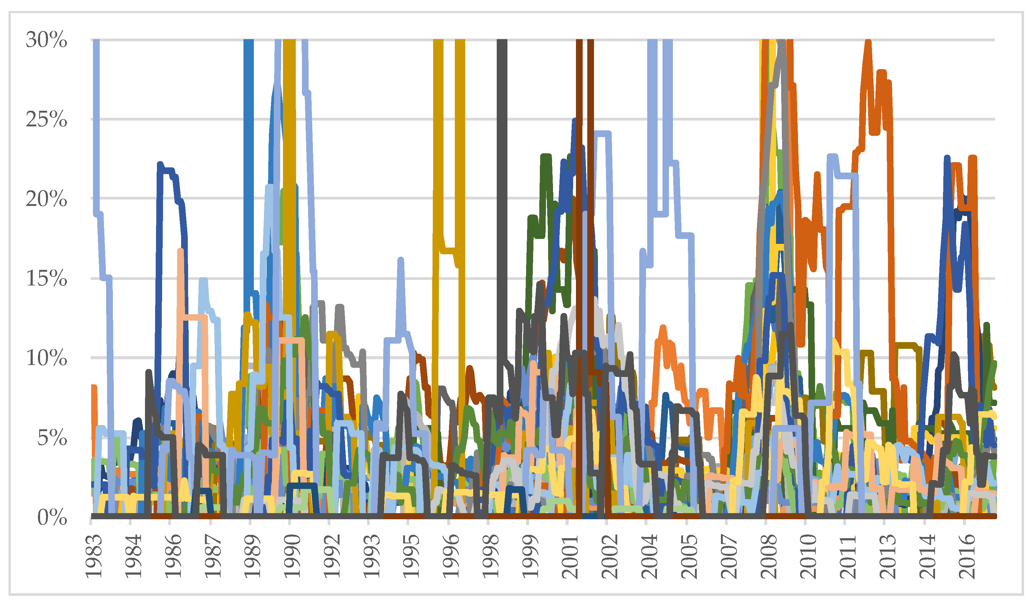
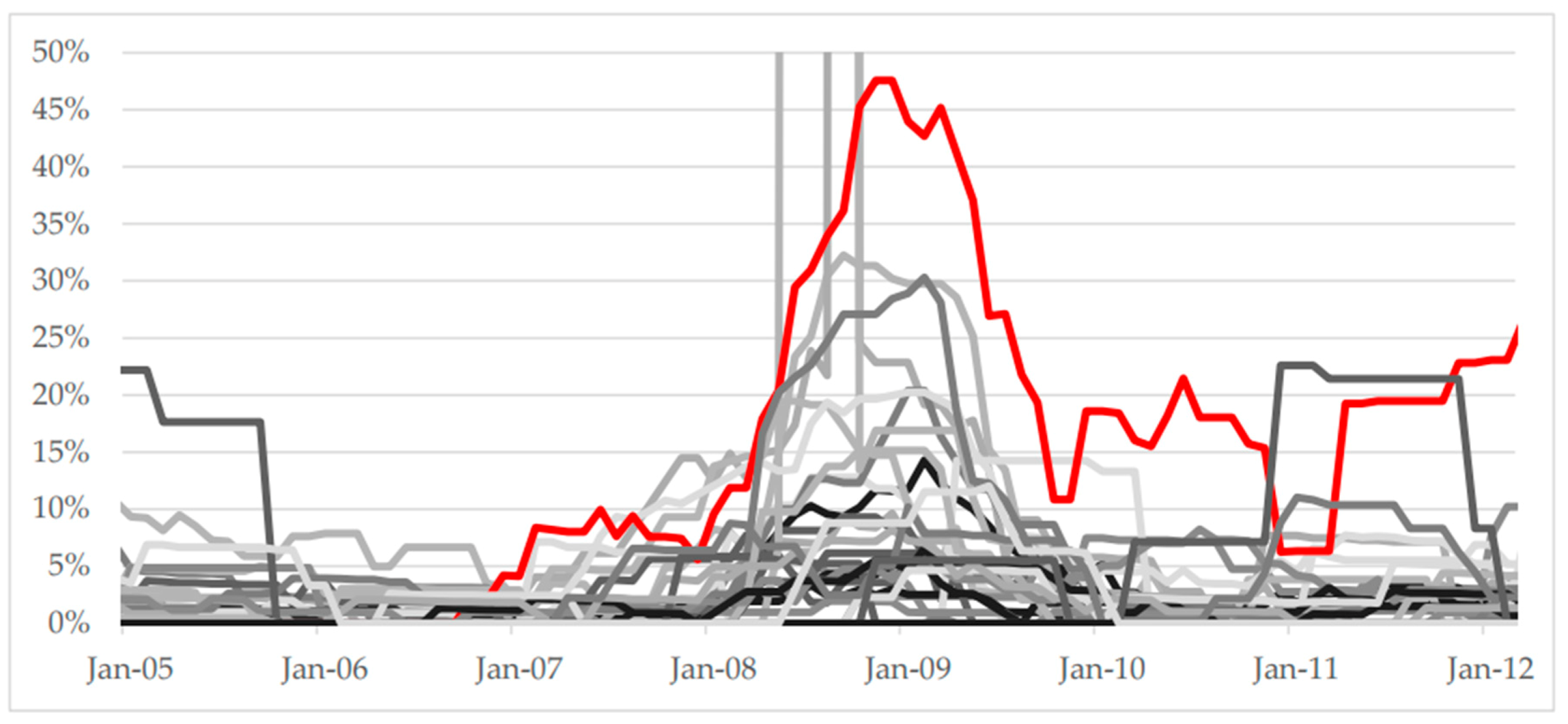
In the context of examining contagion, we might expect sectors that cause contagion to exhibit credit stresses before those stresses then spread to, and are evident in, other sectors. From inspecting the data, there are some sectors that appear to have “led” past downturns in credit quality: that is, corporate default rates jumped in some sectors before default rates across a range of other sectors then subsequently picked up.
For instance, in the August 2007 downturn the default rate in the “media and publishing” sector increased prior to default rates in other sectors. In particular, the default rate for media and publishing reached 8% in 2007 Q1, long before the broader downturn was evident across a wide range of sectors. No other sector saw as early or as sharp a jump in its default rate during 2007; thus, if there was one sector that led others, potentially causing contagion, it would likely have been the media and publishing sector. In
Figure 4, the media and publishing sector is represented by the red line to distinguish this “leading” sector from other corporate sectors during that time period.
This suggests that, if contagion flows from one sector to another, the credit stresses should have originated first in the media and publishing sector before defaults there then triggered credit stresses elsewhere. This is not to say that the media and publishing sector is necessarily more important than others per se—any contagion appears to spread from other sectors in other periods—but it is the sector where credit defaults are evident earliest in the August 2007 episode. As noted later, the identification of the media and publishing sector is not critical for the contagion analysis presented herein; rather, it is meant to serve as an illustration of how contagion testing can be conducted.
The simple test of this contagion in this instance is to examine whether the correlation coefficients between the default rate in the media and publishing sector and default rates in other sectors significantly increased during the “stress” period relative to whole period of data we are considering. In order to do this, we need to define the high and low volatility periods in the sample that we are going to test across for any significant change in correlations.
In this instance, the high volatility period, hereafter referred to as the “stress” period, was assumed to run from January 2008 until January 2011. This was based on when default rates started to increase across many sectors. The low volatility (or “calm”) period was assumed to run from February 2003 until December 2007. The sample period as a whole was therefore defined as the months between February 2003 and January 2011. It is this entire time period from February 2003 to January 2011 that the “benchmark” correlations were calculated over and with which the “stress” correlations were then compared.
It is important to note that, for some sectors, default rates in one of the (sub)sample periods were zero throughout; as such, it is impossible to test for changes in correlation coefficients, because the underlying variance of those particular data series was zero in the (sub)sample which does not allow the calculation of (adjusted) correlation statistics. Of the 32 sectors that could potentially exhibit evidence of contagion from the “media and publishing” sector, it was only possible to conduct the statistical correlation tests for contagion for 29 of them. But, using the sample periods defined above and the sectors for which it was possible to test for changes in correlation coefficients, we can formally test for evidence of contagion in corporate bond markets.
The results, based on tests of simple correlation coefficients, are striking. As shown in the second column of
Table 1, fully 16 of the 29 sectors appeared to show higher correlations in the stress period at the five percent statistical significance level (using a one-sided test, as we are looking for an increase in correlation rather than a decrease). At face value, this appears to be strongly indicative of contagion.
However, when we adjusted the “high stress” correlation coefficients for the underlying bias in the calculation as noted by
Forbes and Rigobon (
2002), this number dropped to just one sector out of the 29 exhibiting signs of contagion, as shown in the fourth column of
Table 1. Furthermore, that sector is where a negative correlation had become less negative (as opposed to an increase in a positive correlation).
From this analysis, it appears that correcting for the bias in correlation coefficients due to the heterogeneous volatility can have a significant impact on the statistical test results of changes in correlation coefficients. Even without the issue of the negative correlation, given the underlying size of the significance test (as opposed to its power) and the number of sectors we are testing, this is not indicative of broad contagion across sectors in corporate bond markets. Consistent with the original work by
Forbes and Rigobon (
2002), this suggests that, while there may be interdependence in credit conditions across different corporate sectors, consistent with them all being affected by a common macro shock, contagion was not formally present in corporate bond markets in the late 2000s based on the results presented above. Instead, the co-movements in default rates are likely to have reflected the common macroeconomic shock, a form of interdependence.
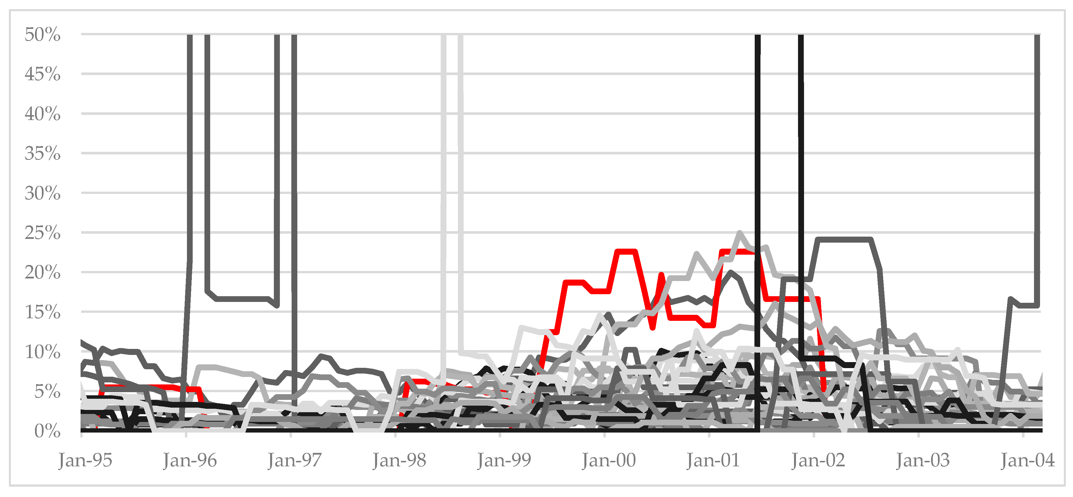
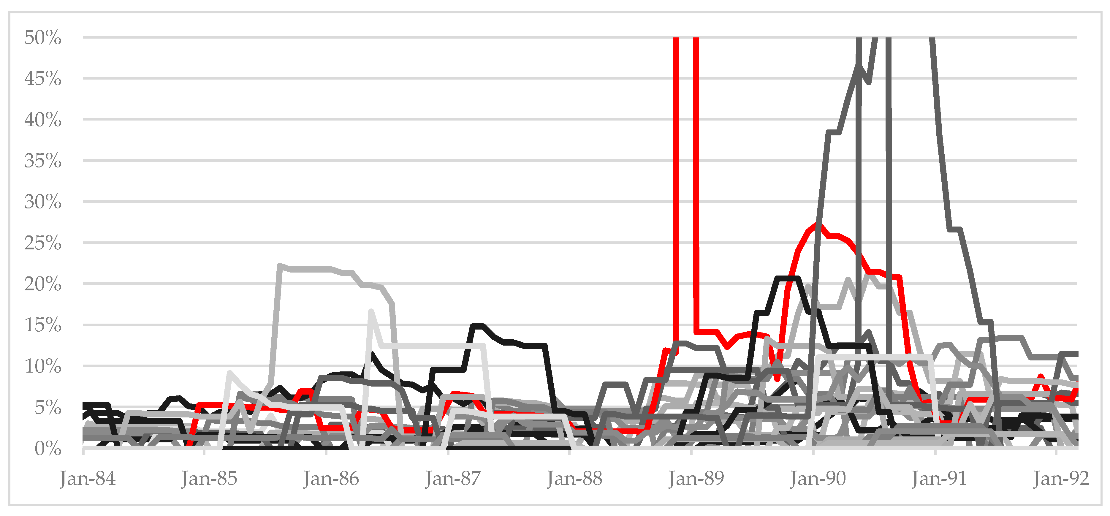
We can conduct the same formal tests for the other two stress periods in the data sample as well; for illustrative purposes, results are presented again based on identifying which sector saw early peaks in default rates. In the early 2000s, the default rate in the “environmental services” sector picked up before default rates in other sectors (
Figure 5), and in the late 1980s’ downturn in credit quality, the “hotels and gaming” sector saw default rates jump before the broader deterioration across a range of sectors (
Figure 6). The fact that these “leading” sectors were not consistent over time could be consistent with each downturn having different underlying drivers or with sectoral performance differing over time or, indeed, with contagion spreading from different sectors in each instance.
As with the previous contagion tests, we again split the subsamples into two periods, each for longer episodes: a “calm” period and a “stress” period. For the early 2000s period illustrated in
Figure 5, the total sample period ran from February 1992 until January 2003; the “stress” episode was assumed to start in July 1999 (with the “calm” period running prior to the “stress” period). For the late 1980s downturn shown in
Figure 6, the total sample period ran from January 1983 until January 1992, with the “stress” period starting in December 1988.
For these earlier two periods in the data, any signs of contagion were less pronounced than in the late 2000s period, even using unadjusted correlation coefficients; in particular, there was very limited evidence of contagion to start with in the late 1980s, although it was more prevalent in the late 1990s downturn. However, it is striking that once the bias in the correlation coefficient was accounted for, the results were now consistent across all three periods in that there was scant genuine evidence of contagion across different corporate bond sectors.
Table 2 summarizes this analysis and illustrates the impact of this bias; it presents the percentage of sectors that exhibit signs of contagion when this is tested for on the basis of both biased and adjusted (unbiased) correlations coefficients. Across the three episodes, co-movements in default rates between the “lead” sectors—highlighted previously for each of the three stress periods in the sample—and other corporate sectors did show evidence of significant changes on the basis of simple correlation statistics. This would suggest some degree of corporate contagion from one sector to another. However, when the bias identified by
Forbes and Rigobon (
1999) was corrected for, any evidence of contagion was sparse at best.
In order to further test the robustness of this result, tests were also run to examine for contagion starting from other sectors: that is, not assuming that contagion would start from those sectors where default rates were observed to jump first (e.g., picking a different starting sector from media and publications in 2008). This is important because, although specific sectors were identified above for illustrative purposes, in principle it is possible that contagion could have flowed from other sectors that had financial fragilities that were not yet fully evident in default rates. However, these broader tests of contagion among different corporate sectors across the same time periods noted above yielded very similar results to those presented in
Table 2—once the bias in correlation coefficients was controlled for, there was very little evidence of contagion across sectors.
To further test the robustness and sensitivity of these results, correlations were also calculated after changing the “calm” and “stress” periods across each of the three episodes in our broader sample. It is possible that the specific choice of these dates could lead to so-called “boundary effects”, where the statistical inference changes when these dates were varied. Happily, this did not appear to be the case, as the broad results presented herein were unchanged; once again, there was little evidence of contagion once the underlying bias in correlation coefficients was controlled for. As with the detailed analytical results presented earlier, unadjusted correlation coefficients gave a misleading picture of potential contagion among sectors and that contagion was not then evident when the bias in the correlation coefficients was adjusted to account for this.

