Abstract
The debate on the UK leaving the European Union is still hot and ongoing today due to many economic, political, social, and other consequences on many different countries over the world. This paper focuses on the reactions of selected Central and Eastern European (CEE) and South and Eastern European (SEE) stock markets to the Brexit vote on 23 June 2016. Using daily data for the time span from January 2010 until July 2016 and the event study methodology (ESM), the return and volatility series are being tested for significant reactions to the Brexit event. The results indicate mixed results regarding the abnormal cumulative return series, but the volatility series were found to be significantly affected by the mentioned event. This is important for international investors and gives information on the reaction of mentioned markets to big political and economic events in order to tailor international portfolios in a way to hedge from risk.
Keywords:
Brexit; stock market reaction; event study; emerging markets; abnormal return; abnormal volatility JEL Classification:
C12; C58; G14
1. Introduction
The debate on the efficient market hypothesis (EMH) of Fama (1965, 1970) is still ongoing today. One of the challenges to the EMH is the different events which influence stock price, return, and volatility movements. Literature has established that more than 300 factors ranging from economic, political, social, etc. influence stock price movements (Harvey et al. 2014). Several major events have been affecting the Europe in the last couple of years, with the controversies of United Kingdom leaving the European Union being one of the most influential ones. Economic consequences of this event (popularly termed Brexit) have been already estimated to be substantial, with total economic costs amounting up to 1.5% of GDP in the third quarter of 2017, and more than 60 billion pounds of those costs amounting by the end of 2018 (Born et al. 2017)1. Since financial markets, and especially stock markets today react strongly to many different events which happen constantly, it remains a difficult task for investors to carry out good2 portfolio management.
Since several major world stock markets have significantly responded to the Brexit vote in 2016 (more details will be provided in the second section), it is important to evaluate the stock market reactions to major political, economic and other events constantly in order to get a clearer picture on what to expect in the future. This is important both for policymakers in order to adjust the (macro)economic policy measures regarding the stability of financial markets and the economy as a whole; but also for (international) investors in the process of portfolio and risk management. The Central and Eastern European (CEE) and South and East European (SEE) stock markets as mostly developing ones are not researched enough in many aspects of portfolio management and finance in general. The effects of the Brexit vote have been explored in the last three years for different stock markets. However, there exists a gap in the academic literature regarding the effects on CEE and SEE markets. The majority of existing research observed how developed markets reacted to the Brexit vote. Since research exists which has shown that CEE and SEE markets are more integrated with developed ones today than before, it is reasonable to assume that effects of the Brexit vote have spilled over to CEE and SEE markets as well. One of the reasons why there exists a gap regarding the mentioned markets could be the smaller liquidity of those markets compared to more developed markets. In that way, the less liquid markets become less popular for investors and for detailed research. Moreover, the CEE and SEE capital markets have less importance for their domestic economies and in corporate finance (see Köke and Schröder 2003). Thus, the purpose of this paper is to empirically evaluate the effects of the Brexit vote on the selected market returns and volatilities. In that way, information can be provided on the efficiency of those markets, as well as how much those markets are connected to the happenings in the Europe. Moreover, in the empirical literature it is found that these markets usually provide somewhat international diversification possibilities. This means that if positive effects of Brexit are found on these markets, international investors could have obtained some hedging investment possibilities on them, due to their (still bit) lower correlations with more developed ones.
The usual approach of the evaluation of such effects in the literature is the event study methodology (ESM) since it has been proven over several decades to be a good tool in finance, and especially in the field of corporate finance. The rest of the paper is structured as follows. Second section gives an overview of the related literature. The third section describes the used methodology in this research, with results being shown in the fourth section. This section deals with the empirical evaluation of the Brexit vote on selected CEE and SEE markets. Discussion on the results is provided in the fifth section with conclusions in the final, sixth section.
2. Previous Related Research
Due to the interest of many parties, including policy makers, investors, and other economic agents involved in the international trade, the effects of the Brexit vote referendum and the British foreign policy are in the focus of many countries, especially the European ones. The academic literature is also focusing on this topic more and more in the last three years. Here are the results of the existing research on this topic regarding the effects of the Brexit vote on global stock markets. One group of authors utilizes the ESM approach in order to evaluate the short-term effects in the next several days after the event on the stock market returns. The second group also examines the Brexit vote effects on return series or volatilities; however, authors here use different approaches (such as regression analysis quantile regression, frequency domain analysis, panel data analysis, etc.).
Quaye et al. (2016) extensively analyzed the effects of the Brexit vote on stock markets, banks, bonds, and other markets over the word by going through newspaper articles and doing a comparative analysis of the values of the indices and prices of different financial assets. Authors report the following: after the Brexit vote, the FTSE 250 dropped by 7.2% the next day, FTSE 100 3.2%, Dow 3.4%, Nasdaq 4.12%, Hang Seng 2.9%, Topix by 7.3%, Euro Stoxx 600 by 7%, ASX 3.2%, DAX by 7%, CAC 8%, and FTMIB 12%. These major indices reacted to a great extent, as well as authors found strong reaction of the British pound exchange rate to other major currencies. Other interesting results can be found in this paper; however, no statistical analysis was performed to evaluate the results via formal testing. The authors mention in the conclusion that ESM can be done in the future work. Amewu et al. (2016) apply the usual ESM approach by using a market model to estimate the abnormal return series for the standardized test and a non-parametric one (the sign test) for the companies listed on the following markets: USA, UK, China, Japan, Germany, and South Africa (the time span is 315 days before the Brexit vote on 23 June 2016 and 15 days after the vote). Only the Chinese market reacted positively to the event; while other markets experienced significant decline in the return series and every market with the exception of the German and UK ones re-bounced to the value before the event day at day +2. Dadurkevicius and Jansonaite (2017) focus on modelling the implied volatility index of the FTSE 100 by using political uncertainty variable, binary variables and the Google search results on the word Brexit. The authors focus also on the companies which are more industry and selling oriented and apply the ESM approach as well. The results indicate that the risk increased before the event due to political uncertainty; the return series differed with their reactions due to different characteristics of sectors to which the returns belonged to. A quantile regression approach with inclusion of the binary variable for the Brexit was used in Bohdalova and Greguš (2017). This research observed bigger European markets (German, French, Irish, Spanish) and bigger emerging ones (Polish and Turkish), with the time span ranging from beginning of 2000 until February 2017. A significant positive effect of the Brexit vote was found in total results, with the greatest impact on the Spanish market and least effects on the Polish. Authors interpret positive results as increasing co-movements between the observed markets. Asymmetric effects of Brexit on individual market returns were found to be significant on different observed quantiles.
Bouoiyour and Selmi (2016) applied a frequency domain causality test and a quantile regression approach to evaluate the effects of uncertainty regarding Brexit on the equity markets of UK, Germany, and France (returns and volatility indices of mentioned markets). Since authors focused on the total uncertainty, Google search results and Twitter tweets regarding the whole process of UK leaving the EU before the Brexit vote, the time span used in the study was January 2010–July 2015. Based upon the results, authors conclude that the German market would suffer the most, followed by French and UK markets. Volatilities and their spillovers were in the focus of Belke et al. (2016). The spillover index, panel and single country SUR (seemingly unrelated regression) regressions are the methodologies applied in this study, where the Brexit effects are observed on the stock returns, sovereign CDS-es (credit default swaps) the 10-year interest rate and the exchange rate (British pound to Euro). The Brexit vote resulted with huge spillovers on financial markets with a magnitude which was never observed before, as authors concluded. Caporale et al. (2018) focused on the FTSE 100 Volatility Index and the volatility indices of exchange rates of British pound the American dollar, Euro and Japanese Yen (period: January 2014 until October 2017). Authors modeled ARMA3 models of the volatility indices with the inclusion of fractal integration in the observed processes and found that in the short run the Brexit vote had a significant impact on all series except the exchange rate to Yen. Alkhatib and Harasheh (2018) apply the ESM approach to the exchange traded funds (ETFs) on London Financial Centre with the event window of −10 to +10 days. The funds have been grouped into several clusters, depending upon the region the ETFs were investing the most (e.g., emerging markets). Using several estimation approaches of the market model, authors obtained results as follows. The emerging markets ETFs gained some returns, as well as the equity-oriented funds. In that way, possibilities to hedge against uncertainty risks regarding the Brexit vote could have been obtained. Kurecic and Kokotovic (2018) applied the unit break tests on 12 stock indices in USA, UK, Russia, China, South America, Hong Kong, Europe, and Japan (range: May 2016–July 2017). Several dates regarding political uncertainty are observed and included in testing for structural breaks in the stock index series, including the Brexit vote. The results indicated that with the exception of the Hang Seng and JSE indices, all other indices exhibited structural breaks on 24 July 2016. Authors concluded that the Brexit vote thus had negative effects on the selected world indices. Burdekin et al. (2018) focused on different stock returns around the world (64 countries) for the period from January until June 2016. Authors used country stock indices and the world market index as a factor to use in the model to estimate the abnormal return series. Authors did not utilize the event study methodology. Instead, they utilized the regression analysis with the inclusion of a binary variable for the date when the Brexit vote was scheduled. The conclusions indicated negative abnormal returns for the majority of the countries analyzed, with PIIGS countries being affected the most. Sultonov and Jehan (2018) focused on Japan’s foreign exchange market and stock markets reactions to Brexit vote (and the US presidential elections). The MGARCH methodology was applied for the return series (for the period 9 February 2016 to 24 March 2017, daily data). Authors calculated differences between the mean returns before and after significant dates, as well the dynamic conditional correlations before and after the events. All of the observed series had a significant change after the events, meaning that uncertain political events reflect on the Japanese stock and foreign exchange markets.
The results are somewhat mixed, with the majority of the research finding that the Brexit vote had a negative effect on global stock market returns, with some hedging possibilities on few stock markets and other financial assets. Since there exists a gap in the literature regarding CEE and SEE countries, this research will focus on those countries in order to obtain first insights.
3. Methodology
The event study methodology is very familiar today for assessing the effects of any type of events on stock returns. In this section we follow Brown and Warner (1980, 1985); Strong (1992); MacKinlay (1997) and Binder (1998) to briefly describe the methodology used in the empirical part of the research. Since we focus on the country market indices and use regional market index as the market factor in the analysis, the notation is as follows. Suppose we have data on actual returns of N stock indices at date t, Ri,t, i ∈ {1, 2, …, N}, t ∈ {1, 2, …, T}. Conditional returns are denoted with E(Ri,t|Ωt), where Ωt denotes available information at date t. The conditional returns are used to evaluate the effects of the event on the stock returns. Thus, abnormal returns ARi,t are calculated as the difference between the realized returns and the conditional ones: ARi,t = Ri,t − E(Ri,t|Ωt); with the conditional return being estimated as the average pre-event widow return, via a market model of some form of asset pricing models (capital asset pricing model, arbitrage pricing theory model, etc.).
Here, we use the following market model in order to estimate the conditional returns as follows: E(Ri,t|Ωt) = αi + βiRm,t + εi,t, where Rm,t denotes the return on the regional market index and the error term is denoted with εi,t, where εi,t ~ N(0, )4. In order to test the hypothesis that the specific event did not had any effects on stock returns, the ARi,t is estimated in the event window. The duration of the event window is usually a short time span in the literature5. In the first step, the average abnormal return is calculated for every date τ in the event window with variances and the cumulative abnormal return is calculated as for each day in the event window. The corresponding variance is and the test value is defined as
The non-parametric tests are often used when the number of stocks in the analysis is small, due to those tests not depending upon the number of stocks. Popular test include the sign test, where the proportion of CARs which are nonnegative is in the focus, i.e., the null hypothesis assumes that p ≤ 0.5, where p = P(CAR ≥ 0). The test value here is defined as
where N+ is the number of nonnegative CARs at date τ. The Wilcoxon (1945) signed rank test focuses on the positive rank of the absolute value of abnormal returns , where the test value at date τ is defined as
Volatility event study focuses on events affecting the volatilities of return series. This is found less often in the event study literature and applications. However, the risk management in the total portfolio management is a very important part. Thus, we test for the hypothesis that the event did not have significant effects on the volatilities of observed returns. Following Agrawal et al. (2003) and Balaban and Constantinou (2006), we firstly estimate the following GARCH (1,1) model for every return series
where Dt,i denotes binary variable equal to 1 day after the event and 0 otherwise. Then, the cross-sectional test for abnormal volatility is performed by calculating the test value
where . Since we observe event window consisting of several days, (4) will be estimated not only with a binary variable being equal to unit value for all of the days after the event.
A Wilcoxon sign test is performed by obtaining the estimated values of volatilities in the pre () and post () event window, as well as for the regional market return ( and ); calculating the ratios and , and apply the test to the pre event and post event ratios.
More details on the event study methodology can be found in Serra (2002); Kothari and Warner (2007) or Kliger and Gurevich (2014) and Conover (1980).
4. Empirical Analysis Results
4.1. Initial Results
The following data was collected from Thomson Reuters in order to empirically evaluate the effects of the Brexit vote: daily data on stock market indices BELEX, BETI, BIRS, BUX, CROBEX, PFTS, PX, SAX, SBITOP, SOFIX, and WIG (corresponding countries: Serbia, Hungary, Bosnia and Herzegovina, Bulgaria, Croatia, Ukraine, Czech Republic, Slovakia, Slovenia, Romania, and Poland respectively) and the regional CEE and SEE6 indices for the period 4 January 2010 up until 8 July 2016. Descriptive statistics for the common sample is given in Appendix A in Table A1. In total, 1630 observations are available for every series. We use daily data since Brown and Warner (1985) showed that daily data provide just as well-specified results of standard parametric test as monthly data does. Firstly, we calculated the return values on the day after the Brexit vote (23 June 2016) in order to get initial insight into the movements on the mentioned markets. The following returns were calculated: −1.8% BELEX, −3.59% BETI, −0.2% BIRS, −4.56% BUX, −1.67% CROBEX, −0.24%PFTS, −4.36% PX, 0.01% SAX, −2.18% SBITOP, −1.14% SOFIX, and −4.48% WIG. Every index dropped with the exception of the Slovak index.
In the first step, we estimate the market model in the pre event window and obtain the estimated values of return series for every stock market by using CEE and then SEE index returns as an explanatory variable. Then, in the second step, the length of the event window is chosen to be 21 days (−10 to +10 days) and we calculate the test values regarding the return series (θ1, θ2 and θ3). The event day of the Brexit vote was 23 June 2016, and this is depicted as day 0 in all of the following tables and graphs. The results are shown in Table 1 (CEE factor) and Table 2 (SEE factor).

Table 1.
Stock market reactions to Brexit, CEE regional factor.
Table 2.
Stock market reactions to Brexit, SEE regional factor.
The results in Table 1 indicate that no effects regarding the observed markets were found to be significant if the CEE regional index is used as the market factor. Although, the was found to be negative four days after the Brexit vote, with more than double the value of the at 23 June 2016. However, as stated, the results are not significant. All of the return series were found nonsignificant for the days before the event as well. This could be interpreted that investors did not spread out some beliefs and rumors, and thus did not generate abnormal gains or losses. The results are always the same based upon all three test statistics.
The conclusion is a bit different if we use the SEE regional market, in Table 2. The becomes positive the day after the event and after day +3 becomes statistically significant. However, the first three s were not significant. Since the majority of previous event study methodology literature focuses on a narrow window, from 1 day to a maximum 5 days, the results in Table 2 which refer to those days which are more distant to the day 0 could be observed as being result from other factors and not the Brexit vote per se. Again, the conclusions about the tested hypothesis are the same based upon all three test statistics.
Graphical representations of the s for the CEE and SEE factor are given on Figure 1 and Figure 2, with the 95% confidence intervals (CIs), for a better overview of the movement of the average cumulative abnormal return. The conclusion is again the same as it was in Table 1 and Table 2.
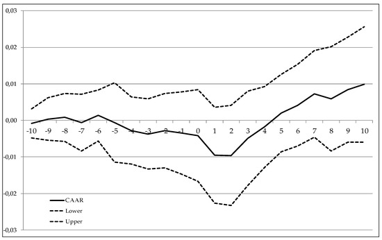
Figure 1.
for all markets, CEE regional market factor, with 95% CIs.
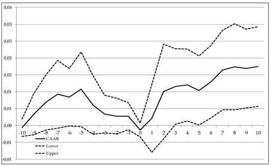
Figure 2.
for all markets, SEE regional market factor, with 95% CIs.
Effects on volatility have been examined as well with the results given in Table 3. Firstly, the test statistic θ4 was calculated for one day after the event and then for all 10 days after the event at day 0. Both test statistics indicate the non-rejection of the null hypothesis, meaning that no significant abnormal volatilities were found due to the Brexit vote. By applying the non-parametric Wilcoxon test, it can be seen that only the volatility on the +1 day was significantly different from the pre-event volatility. This is weak evidence in favor of Brexit affecting the volatility on the examined markets.
Table 3.
Volatility reaction results to Brexit.
4.2. Robustness Checking
The robustness checking of the results was performed by changing the length of the event window. Since shorter time spans are observed within this methodology, we opted to use −3 to +3 days for the event window. Thus, as in Table 1 and Table 2, we perform the same tests, but for the shorter event window, with the results shown in Table 4 and Table 5. By focusing on Table 4, the results are the same as in Table 1, with no significant effects found in all three days after the event even though the cumulative abnormal returns get more negative. However, the results become a bit different by observing Table 5 with the SEE regional factor. Now, the results are significant in days before and after the event, with the exception on day +2.
Table 4.
Stock market reactions to Brexit, CEE regional factor, three-day window length.
Table 5.
Stock market reactions to Brexit, SEE regional factor, three-day window length.
The volatility event study for the +3 days results are shown in Table 6. As it can be seen, the test results indicate significant effects on the volatility for the non parametric test for both regional factors, which confirms the short term results of +1 day from Table 3. Thus, there is more evidence in favor of Brexit vote affecting volatilities on the observed stock markets compared to return series.
Table 6.
Volatility reaction results to Brexit, +3 days event window length.
5. Discussion
Several conclusions based upon the obtained results in the previous section can be provided. Firstly, by focusing on the CEE regional factor as a ‘market’ return for the observed countries, the result indicated no significant effects on the abnormal return series. Both the parametric and non-parametric tests confirmed this conclusion. This was found to be true both for the event window length of 21 (−10 to +10) days and 7 (−3 to +3) days. Although the results were nonsignificant, the abnormal returns did fell after the Brexit vote (after day 0) and it took about three days to rebound to the value before the vote. The volatility was somewhat affected due to significant results of the Wilcoxon test for day +1. These results became insignificant for the window length of +10 days, meaning that the effects were extremely short termed. Those effects on volatilities were found present for the +3 day period. Thus, in the three days after the 23 June 2016, there was excessive volatility on the observed markets, with some insignificant negative cumulative abnormal returns.
Secondly, if we focus on the SEE regional factor in the analysis, the results are somewhat different. The abnormal return series, although insignificant, become positive in the next three days after the event, compared to the previous factor in the analysis. Moreover, the return series become significant on the third day and stay that way until the end of +10 window length. However, it could be said that this is not due to the Brexit vote itself, because it would mean that investors had a delayed reaction to the happenings around the whole political uncertainty. The results become significant for days before and after the event when the length of the event window was shortened to −3 to +3, with the exception of the day +2. Here, all of the cumulative abnormal returns were negative, with becoming positive on day +2. This is more in line with the CEE results of negative returns. Thus, some weak evidence exists on Brexit vote affecting the observed markets. Finally, the volatilities test in the SEE factor framework also confirms that excessive volatility existed around the crucial date.
Thus, some mixed results were obtained regarding the return series. This is due to changing the regional factor as the one describing the individual country returns. Since the major conclusion is that volatilities were significantly different on those markets before and after the event, it could be said that some effects of the Brexit vote spilled over to the CEE and SEE markets as well. This is important for international investors who are focused on risk hedging. Since the volatilities have gone up in the post event period, this is not favorable for the risk management goals. This is not surprising, due to previous literature finding that the mentioned markets are today more integrated with the more developed markets (e.g., see Kizys and Pierdzioch 2011 or Fronc and Mielus 2017).
6. Conclusions
The rising political and economic uncertainties around the world affect the stock markets and their participants. The extent to which this is true is important for the policy makers and investors around the world. Timely decisions are crucial for good conduction of economic policies and portfolio management in order to obtain the best possible results. This paper focused on an example of a big political and economic event and its effects on the CEE and SEE stock markets. Since previous literature identifies such markets as being those where some opportunities for international diversification exists, it is important to obtain information on how those markets react to big events. Major results indicate that somewhat mixed results are found on the return series (negative abnormal cumulative returns but nonsignificant) and significant results were found in the volatilities (greater volatilities in the short term after the Brexit vote).
Some of the shortcomings in this research included the following ones. We observed only one event, the Brexit day vote referendum. However, this was made due to getting first insights into whether the biggest events affect the aforementioned markets. If it was found that the biggest events do not affect the markets at all, it is questionable if other minor events leading up to (or after the main event) even could have meaningful impacts. Thus, future work should extend the analysis by observing other political and economic events regarding the whole uncertainty in the European Union regarding the UK’s leaving it. Moreover, due to different conclusions regarding the abnormal return testing because using different market factors in the model, future work could extend the model and augment it with other market factors to see if changes in results will occur.
Since this is, to the knowledge of the author, the first study which focuses on selected CEE and SEE markets and their reactions to the Brexit uncertainties, we hope that it will invoke more future analysis regarding these markets and possibilities they could or could not provide for international investors regarding other political and economic events, especially those regarding the problems of EU.
Funding
This research received no external funding. The APC was funded by institutions through the Knowledge Unlatched initiative and partially funded by MDPI.
Acknowledgments
Author would like to thank two anonymous referees for their valuable comments and suggestions which contributed to the quality of the paper.
Conflicts of Interest
The author declares no conflict of interest.
Appendix A

Figure A1.
Individual s, CEE regional market factor.

Figure A2.
Individual s, SEE regional market factor.
Table A1.
Descriptive statistics for return series.
Table A1.
Descriptive statistics for return series.
| Return | Mean | Median | Max | Min | Std. dev. |
|---|---|---|---|---|---|
| BELEX | 0.00043 | 0.00019 | 0.08229 | −0.07408 | 0.00858 |
| BETI | 0.00065 | 0.00044 | 0.09088 | −0.06968 | 0.01061 |
| BIRS | −0.00029 | 0.00000 | 0.03842 | −0.04166 | 0.00678 |
| BUX | 0.00022 | 0.00019 | 0.05515 | −0.06984 | 0.01274 |
| CEE | 0.00009 | 0.00024 | 0.05557 | −0.06239 | 0.01327 |
| CROBEX | 0.00000 | 0.00003 | 0.08563 | −0.02886 | 0.00670 |
| PFTS | 0.00023 | 0.00019 | 0.12265 | −0.07494 | 0.01482 |
| PX | 0.00059 | 0.00057 | 0.05222 | −0.05183 | 0.01169 |
| SAX | 0.00069 | 0.00010 | 0.09118 | −0.06053 | 0.01114 |
| SBITOP | 0.00015 | 0.00016 | 0.03721 | −0.06059 | 0.00920 |
| SEE | 0.00026 | 0.00040 | 0.03880 | −0.03913 | 0.00669 |
| SOFIX | 0.00027 | 0.00034 | 0.03809 | −0.04497 | 0.00833 |
| WIG | 0.00022 | 0.00056 | 0.04105 | −0.06086 | 0.01011 |
Table A2.
GARCH estimation results, binary variable only day after event.
Table A2.
GARCH estimation results, binary variable only day after event.
| Variance | ||||
|---|---|---|---|---|
| BELEX | 4.48 × 10⁻⁶ (0.000) *** | 0.179 (0.000) *** | 0.764 (0.000) *** | 9.96 × 10⁻⁵ (0.467) |
| BETI | 4.72 × 10⁻⁶ (0.000) *** | 0.129 (0.000) *** | 0.830 (0.000) *** | 0.0003 (0.318) |
| BIRS | 1.49 × 10⁻⁶ (0.164) | 0.065 (0.077) * | 0.961 (0.000) *** | 5.20 × 10⁻⁵ (0.747) |
| BUX | 4.01 × 10⁻⁶ (0.008) *** | 0.053 (0.000) *** | 0.922 (0.000) *** | 0.0003 (0.271) |
| CROBEX | 9.99 × 10⁻⁷ (0.006) *** | 0.070 (0.000) *** | 0.906 (0.000) *** | 6.18 × 10⁻⁵ (0.280) |
| PFTS | 0.0001 (0.000) *** | 0.133 (0.000) *** | 0.465 (0.000) *** | −0.0003 (0.000) *** |
| PX | 3.42 × 10⁻⁶ (0.009) *** | 0.072 (0.000) *** | 0.902 (0.000) *** | 0.001 (0.318) |
| SAX | 8.48 × 10⁻⁶ (0.010) ** | 0.124 (0.004) *** | 0.543 (0.001) *** | −0.0002 (0.000) *** |
| SBITOP | 9.73 × 10⁻⁶ (0.000) *** | 0.199 (0.000) *** | 0.707 (0.000) *** | 0.0002 (0.498) |
| SOFIX | 8.24 × 10⁻⁶ (0.000) *** | 0.218 (0.000) *** | 0.679 (0.000) *** | 4.41 × 10⁻⁵ (0.751) |
| WIG | 2.92 × 10⁻⁶ (0.005) *** | 0.069 (0.000) *** | 0.903 (0.000) *** | 0.0002 (0.308) |
Note: GARCH models have been estimated with the assumption of t-distribution of error term. p-values are given in parenthesis.
Table A3.
GARCH estimation results, binary variable for 10 days after the event.
Table A3.
GARCH estimation results, binary variable for 10 days after the event.
| Variance | ||||
|---|---|---|---|---|
| BELEX | 4.11 × 10⁻⁶ (0.000) *** | 0.165 (0.000) *** | 0.783 (0.000) *** | −7.13 × 10⁻⁶ (0.100) |
| BETI | 4.39 × 10⁻⁶ (0.000) *** | 0.124 (0.000) *** | 0.840 (0.000) *** | −1.59 × 10⁻⁵ (0.100) |
| BIRS | 1.51 × 10⁻⁶ (0.163) | 0.065 (0.077) * | 0.961 (0.000) *** | 2.82 × 10⁻⁵ (0.522) |
| BUX | 3.94 × 10⁻⁶ (0.009) *** | 0.053 (0.000) *** | 0.923 (0.000) *** | −1.60 × 10⁻⁵ (0.247) |
| CROBEX | 1.02 × 10⁻⁶ (0.006) *** | 0.069 (0.000) *** | 0.907 (0.000) *** | 6.41 × 10⁻⁶ (0.447) |
| PFTS | 1.52 × 10⁻⁵ (0.000) *** | 0.295 (0.000) *** | 0.706 (0.000) *** | −1.40 × 10⁻⁵ (0.141) *** |
| PX | 3.49 × 10⁻⁶ (0.009) *** | 0.073 (0.000) *** | 0.901 (0.000) *** | 0.0001 (0.145) |
| SAX | 8.40 × 10⁻⁵ (0.000) *** | 0.142 (0.000) *** | 0.223 (0.025) ** | −5.36 × 10⁻⁵ (0.000) *** |
| SBITOP | 9.77 × 10⁻⁶ (0.000) *** | 0.199 (0.000) *** | 0.708 (0.000) *** | 1.19 × 10⁻⁵ (0.589) |
| SOFIX | 8.14 × 10⁻⁶ (0.000) *** | 0.215 (0.000) *** | 0.684 (0.000) *** | −1.84 × 10⁻⁶ (0.875) |
| WIG | 2.82 × 10⁻⁶ (0.005) *** | 0.070 (0.000) *** | 0.904 (0.000) *** | −1.44 × 10⁻⁵ (0.297) |
Note: GARCH models have been estimated with the assumption of t-distribution of error term. p-values are given in parenthesis.
Table A4.
GARCH estimation results, binary variable for three days after the event.
Table A4.
GARCH estimation results, binary variable for three days after the event.
| Variance | ||||
|---|---|---|---|---|
| BELEX | 4.25 × 10⁻⁶ (0.000) *** | 0.174 (0.000) *** | 0.773 (0.000) *** | 0.0001 (0.460) |
| BETI | 4.52 × 10⁻⁶ (0.000) *** | 0.127 (0.000) *** | 0.834 (0.000) *** | 0.0004 (0.361) |
| BIRS | 1.52 × 10⁻⁶ (0.163) | 0.065 (0.074) * | 0.961 (0.000) *** | 9.00 × 10⁻⁶ (0.906) |
| BUX | 3.91 × 10⁻⁶ (0.008) *** | 0.053 (0.000) *** | 0.923 (0.000) *** | 0.001 (0.355) |
| CROBEX | 1.00 × 10⁻⁶ (0.006) *** | 0.070 (0.000) *** | 0.906 (0.000) *** | 5.81 × 10⁻⁵ (0.283) |
| PFTS | 0.0001 (0.000) *** | 0.136 (0.000) *** | 0.474 (0.000) *** | −0.0002 (0.963) |
| PX | 3.37 × 10⁻⁶ (0.009) *** | 0.072 (0.000) *** | 0.903 (0.000) *** | 0.001 (0.376) |
| SAX | 8.32 × 10⁻⁵ (0.000) *** | 0.139 (0.000) *** | 0.231 (0.021) ** | −8.33 × 10⁻⁵ (0.000) *** |
| SBITOP | 9.78 × 10⁻⁶ (0.000) *** | 0.201 (0.000) *** | 0.706 (0.000) *** | 7.95 × 10⁻⁵ (0.474) |
| SOFIX | 3.61 × 10⁻⁵ (0.000) *** | 0.142 (0.000) *** | 0.567 (0.000) *** | −5.25 × 10⁻⁵ (0.000) *** |
| WIG | 2.84 × 10⁻⁶ (0.005) *** | 0.069 (0.000) *** | 0.904 (0.000) *** | 0.0004 (0.294) |
Note: GARCH models have been estimated with the assumption of t-distribution of error term. p-values are given in parenthesis.
References
- Agrawal, Deepak, Sreedhar Bhatrah, and Siva Viswanthan. 2003. Technological Change and Stock Return Volatility: Evidence from eCommerce Adoptions. Available online: http://dx.doi.org/10.2139/ssrn.387543 (accessed on 2 January 2019).
- Alkhatib, Akram, and Murad Harasheh. 2018. Performance of Exchange Traded Funds during the Brexit Referendum: An Event Study. International Journal of Financial Studies 6: 64. [Google Scholar] [CrossRef]
- Amewu, Godfred, Jones Odei Mensah, and Paul Alagidede. 2016. Reaction of global stock markets to Brexit. Journal of African Political Economy & Development 1: 40–55. [Google Scholar]
- Balaban, Ercan, and Charalambos Constantionu. 2006. Volatility clustering and event-induced volatility: Evidence from UK mergers and acquisitions. The European Journal of Finance 12: 449–53. [Google Scholar] [CrossRef]
- Belke, Ansgar, and Sebastian Ptok. 2018. British-European Trade Relations and Brexit: An Empirical Analysis of the Impact of Economic and Financial Uncertainty on Exports. International Journal of Financial Studies 6: 73. [Google Scholar] [CrossRef]
- Belke, Ansgar, Irina Dubova, and Thomas Osowoski. 2016. Policy Uncertainty and International Financial Markets: The Case of Brexit. ROME Discussion Paper Series. Discussion Paper Series No 2016-07. CEPS Working Document No. 429. Available online: https://www.ceps.eu/publications/policy-uncertainty-and-international-financial-markets-case-brexit (accessed on 22 January 2019).
- Binder, John. 1998. The event study methodology since 1969. Review of Quantitative Finance and Accounting 11: 111–37. [Google Scholar] [CrossRef]
- Bohdalova, Maria, and Michal Greguš. 2017. The Impacts of Brexit on European Equity Markets. Financial Assets and Investing 8: 5–18. [Google Scholar] [CrossRef]
- Born, Benjamin, Gernot Müller, Moritz Schularick, and Petr Sedlaček. 2017. The Economic Consequences of the Brexit Vote. Discussion Papers 1738. London, UK: Centre for Macroeconomics (CFM). [Google Scholar]
- Bouoiyour, Jamal, and Refk Selmi. 2016. Is Uncertainty over Brexit Damaging the UK and European Equities? MPRA Paper No. 70520. Munich: University Library of Munich. [Google Scholar]
- Brown, Stephen, and Jerlod Warner. 1980. Measuring security price performance. Journal of Financial Economics 8: 205–58. [Google Scholar] [CrossRef]
- Brown, Stephen, and Jerlod Warner. 1985. Using daily stock returns: The case of event studies. Journal of Financial Economics 14: 3–31. [Google Scholar] [CrossRef]
- Bruno, Radolph, Nauro Campos, Saul Estrin, and Meng Tian. 2016. Gravitating towards Europe: An Econometric Analysis of the FDI Effects of EU Membership. CEP Technical Paper, Brexit Analysis No 3. ETH-Zurich and IZA-Bonn. Available online: http://cep.lse.ac.uk/pubs/download/brexit03_technical_paper.pdf (accessed on 22 January 2019).
- Burdekin, Richard, Eric Hugson, and Jinlin Gu. 2018. A first look at Brexit and Global Equity Markets. Applied Economic Letters 25: 136–40. [Google Scholar] [CrossRef]
- Busch, Berthold, and Matthes Jürgen. 2016. Brexit—The Economic Impact: A Meta-Analysis. IW-Reports 10/2016. Köln: Institut der deutschen Wirtschaft (IW)/German Economic Institute. [Google Scholar]
- Caporale, Guglielmo Maria, Luis Gil-Alana, and Tommaso Trani. 2018. Brexit and Uncertainty in Financial Markets. International Journal of Financial Studies 6: 21. [Google Scholar] [CrossRef]
- Centre for European Policy Studies. 2017. An Assessment of the Economic Impact of Brexit on the EU 27. Study for the IMCO Committee. Brussels: CEPS. [Google Scholar]
- Conover, William Jay. 1980. Practical Nonparametric Statistics, 2nd ed. New York: Wiley. [Google Scholar]
- Dadurkevicius, Mindaugas, and Adele Jansonaite. 2017. Effects of Prescheduled Political Events on Stock Markets: The Case of Brexit. SSE Riga Student Research Papers 2017: 11 (198). Available online: https://www.sseriga.edu/sites/default/files/2018-08/11Paper_Dadurkevicius_Jansonaite.pdf (accessed on 2 January 2019).
- Dhingra, Swati, Gianmarco Ottaviano, Thomas Sampson, and John Van Reenen. 2016. The Impact of Brexit on Foreign Investment in the UK. CEP Brexit Analysis No 3. Available online: http://cep.lse.ac.uk/pubs/download/brexit03.pdf (accessed on 2 January 2019).
- Fama, Eugene. 1965. The Behavior of Stock Market Prices. The Journal of Business 38: 4–105. [Google Scholar] [CrossRef]
- Fama, Eugene. 1970. Efficient Capital Markets: A Review of Theory and Empirical Work. The Journal of Finance 25: 383–417. [Google Scholar] [CrossRef]
- Wilcoxon, Frank. 1945. Individual comparison by ranking methods. Biometrics Bulletin 1: 80–83. [Google Scholar] [CrossRef]
- Fronc, Michal, and Piotr Mielus. 2017. Financial convergence on emerging markets: The case of CEE countries. Bank i Kredyt 48: 149–72. [Google Scholar]
- Harvey, Campbell, Yan Liu, and Heqing Zhu. 2014. … and the Cross-Section of Expected Returns. Working paper. Durham, NC, USA: Duke University. [Google Scholar]
- Holler, Jochen. 2004. Event Study-Methodik und statistische Signifikanz (Banking, Finance & Accounting Research Series). Oldenburg: WIR. [Google Scholar]
- Kizys, Renatas, and Christian Pierdzioch. 2011. The Financial Crisis and the Stock Markets of the CEE Countries. Czech Journal of Economics and Finance 61: 153–72. [Google Scholar]
- Kliger, Doron, and Gregory Gurevich. 2014. Event Studies for Financial Research. New York: Palgrawe MacMillan. [Google Scholar]
- Köke, Jens, and Michael Schröder. 2003. The Prospects of Capital Markets in Central and Eastern Europe. Eastern European Economics 41: 5–37. [Google Scholar] [CrossRef]
- Kothari, Sriprakash, and Jerold Warner. 2007. Econometrics of Event Studies. In Handbook of Corporate Finance—Empirical Corporate Finance. Edited by B. Espen Eckbo. Amsterdam: Elsevier, vol. 1. [Google Scholar]
- Kurecic, Petar, and Filip Kokotovic. 2018. Empirical analysis of the impact of Brexit referendum and post-referendum events on selected stock exchange indices. South East European Journal of Economics and Business 13: 7–16. [Google Scholar] [CrossRef]
- MacKinlay, Craig. 1997. Event Studies in Economics and Finance. Journal of Economic Literature 35: 13–39. [Google Scholar]
- Newey, Whitney, and Kenneth West. 1987. A Simple, Positive Semi-definite, Heteroskedasticity and Autocorrelation Consistent Covariance Matrix. Econometrica 55: 703–8. [Google Scholar] [CrossRef]
- OECD. 2018a. Available online: https://stats.oecd.org/glossary/detail.asp?ID=303 (accessed on 2 January 2019).
- OECD. 2018b. Available online: http://www.oecd.org/south-east-europe/economies/ (accessed on 2 January 2019).
- Quaye, Isaac, Mu Yinping, Braimah Abudu, and Ramous Agyare. 2016. Review of Stock Markets’ Reaction to New Events: Evidence from Brexit. Journal of Financial Risk Management 5: 281–314. [Google Scholar] [CrossRef]
- Serra, Ana Paula. 2002. Event Study Tests. A Brief Survey. Working papers Da Fep, Investigação—Trabalhos em curso—nº 117, Maio de. 2002. Working Papers da FEP no. 117. Porto, Portugal: School of Economics and Management of the University of Porto. [Google Scholar]
- Sheskin, David. 2004. Handbook of Parametric and Nonparametric Statistical Procedures. Boca Raton: CRC Press. [Google Scholar]
- Simionescu, Mihaela. 2018. The impact of Brexit on the UK inwards FDI. Sustainability 3: 6–20. [Google Scholar] [CrossRef]
- Strong, Norman. 1992. Modelling abnormal returns: a review article. Journal of Business Finance & Accounting 19: 533–53. [Google Scholar] [CrossRef]
- Sultonov, Mirzosaid, and Shahzadah Nayyar Jehan. 2018. Dynamic Linkages between Japan’s Foreign Exchange and Stock Markets: Response to the Brexit Referendum and the 2016 U.S. Presidential Election. Journal of Risk and Financial Management 11: 34. [Google Scholar] [CrossRef]
- White, Halbert. 1980. A heteroskedasticity-consistent covariance matrix estimator and direct test for heteroskedasticity. Econometrica 48: 285–316. [Google Scholar] [CrossRef]
| 1 | Several other implications and estimations on the effects on different (macro)economic variables can be found in: Bruno et al. (2016), Dhingra et al. (2016) or Simionescu (2018) for FDI effects; Belke and Ptok (2018) for trade consequences; CEPS (2017) for total economic costs for UK and EU 27. Other estimated consequences are reviewed in a meta study of Busch and Jürgen (2016). |
| 2 | Good in terms of achieving desired investment goals. |
| 3 | Autoregressive Moving Average. |
| 4 | If there exists autocorrelation and/or heteroskedasticity in the data, the least squares method of estimation of conditional returns can be augmented with White (1980) corrected standard errors or Newey and West (1987) corrections. Details are given in Kliger and Gurevich (2014). |
| 5 | Sheskin (2004) explains that shorter time span tests in the event study approach have more power of test compared to longer time spans. Holler (2004) denotes that the event window typically varies from 1 to 11 days. |
| 6 | Since OECD (2018a, 2018b) classifies some of the countries as CEE and SEE markets simultaneously, we opted to do the whole procedure for both regional indices as “market” indices. |
© 2019 by the author. Licensee MDPI, Basel, Switzerland. This article is an open access article distributed under the terms and conditions of the Creative Commons Attribution (CC BY) license (http://creativecommons.org/licenses/by/4.0/).