The Behaviour of the Equity Yield and Its Relation with the Bond Yield: The Role of Inflation

Abstract

Understanding the behaviour of the equity yield and its relation to the bond yield is important for portfolio managers and those engaged in modelling the interaction between asset classes. During the mid-1900s, the equity yield—which was previously greater than the bond yield—declined, while the bond yield rose and became higher. Research, seeking to understand this, put forward the view that stock and bond return volatility is key. Evidence from the 2000s suggest that the relative values of the equity and bond yield have flipped again, with the former now greater. Empirical evidence presented here shows that during such periods, the hypothesised relation between the equity yield and the bond yield and the two volatilities also changes, with the signs reversed. Moreover, there is noticeable variation in the coefficient values. This paper argues that the relative equity and bond yield values are, to a large extent, driven by inflation volatility. High inflation volatility persisted during the first half of the twentieth century when the equity yield was higher. This was followed by more benign inflation volatility when the bond yield became higher. Evidence for a long span of US data, and shorter German, Japanese, and UK data, suggests the recent rise in the equity yield is accompanied by an uptick in inflation volatility relative to its recent tranquillity.

1. Introduction

The nature of the relation between stocks and bonds remains of important interest to academics, investors, and policy-makers (see, for example, Shiller and Beltratti 1992; Campbell and Ammer 1993; Baele et al. 2010; Campbell et al. 2017). The correlation between these assets underpins the Fed model that can be used (perhaps controversially) to predict subsequent stock returns (see, for example, Asness 2003; Bekaert and Engstrom 2010; Maio 2013), while large movements in the relation are ascribed to changes in investors behaviour, such as flight-to-safety effects (e.g., Hakkio and Keeton 2009; Chiang et al. 2015). The nature of the stock and bond relation may, thus, be an indicator of the relative health of these markets and the underlying economy.

Using the framework introduced by (Asness 2000), we examine the nature of the relation between stocks and bonds. This analysis is pertinent, given the past 30 years have been marked by falling interest rates together with significant stock market bull runs during the 1990s and 2010s. Examining the history of movements between stocks and bonds, prior to the mid-1950s, the dividend yield was higher than the yield on 10-year Government bonds; after this date, the position was reversed, with the bond yield higher than the dividend yield. Since the beginning of the 2010s, the two yields have converged. A similar picture can be seen in the relation between the earnings yield and bond yields. A higher earnings yield could be observed prior to approximately 1970, after which the two yields are of a similar value. However, since the beginning of the 2010s, we again see the earnings yield notably higher than the bond yield. Understanding why these changes take place remains a key question in portfolio management, and with respect to our knowledge of the interaction between markets.

We use the framework of Asness (2000), who argues that movements in the equity yield (either dividends or earnings) are driven by movements in the bond yield, to which they are positively related, and movements in relative stock and bond return volatility. Specifically, the equity yield is increasing in stock volatility and decreasing in bond volatility. Moreover, Asness argues that it is the recent history and experiences of investors with respect to volatility that is important. We reconsider this model in trying to understand the current state of the relation between stocks and bonds and, notably, the apparent recent switch in the relative values of equity and bond yields.

We begin by updating the regression model results of Asness using a long span of data for the United States. However, our greater interest is in the potential for variation in the nature of the estimated relations, including structural breaks and time-variation, as well as variation across quantiles of the dependent variable. Of note, we uncover periods where the regression coefficients flip sign, such that the bond yield and stock volatility have a negative relation with the equity yield and, likewise, bond volatility has a positive association. Further, we argue that the behaviour of inflation also plays a pivotal role in moving the equity yield. We observe that inflation exhibits a high level of volatility in the early part of the sample when the equity yield is greater than the bond yield. Further, the switch to the bond yield being higher than the equity yield is consistent with the period when inflation volatility falls. Inflation has been relatively tranquil over the most recent past, however, an uptick in volatility, we argue, is consistent with the equity yield again moving higher than the bond yield. In addition to the evidence for a long history of US data, we also consider a shorter history for Germany, Japan, and the United Kingdom in seeking to provide robust evidence for this view.

2. Full Sample Regression

Asness (2000) argues that the relation between the yield on earnings and bonds is driven by the relative volatilities of stocks and bonds. Asness argues that the expected return on stocks is given by the Campbell and Shiller (1988) present value model, while the return on bonds is determined by the bond yield. Asness then argues that stock and bond returns are linked through their long-run volatilities, such that the difference between stock and bond returns increase when the difference in their respective volatilities also increases. This produces the following regressions for the dividend/price (d/p) and earnings/price (e/p) ratios:

(d/p)_t = α + β Y_t + γ σ_s,t + λ σ_b,t + ε_t,

(1)

(e/p)_t = α + β Y_t + γ σ_s,t + λ σ_b,t + ε_t,

(2)

where the d/p and e/p series are determined by long-term government bond yields, Y, and the volatility of stock, σ_s,t, and bond, σ_s,t, returns. The expectation is that the coefficient values will take the following signs: β > 0; γ > 0; λ < 0. This indicates that the yield on stocks will increase with the yield on long-term government bonds and the volatility of stock returns, and decrease with the volatility of bond returns.

We obtain monthly data over the period 1900m1 to 2018m5. These data (and other data used in the study) are obtained from a combination of the St Louis Federal Reserve FRED database, the website of Robert Shiller, and DataStream. Specifically, we have data on prices, dividends, and earnings on the S&P Composite index and 10-year Treasury bond index returns and yields. 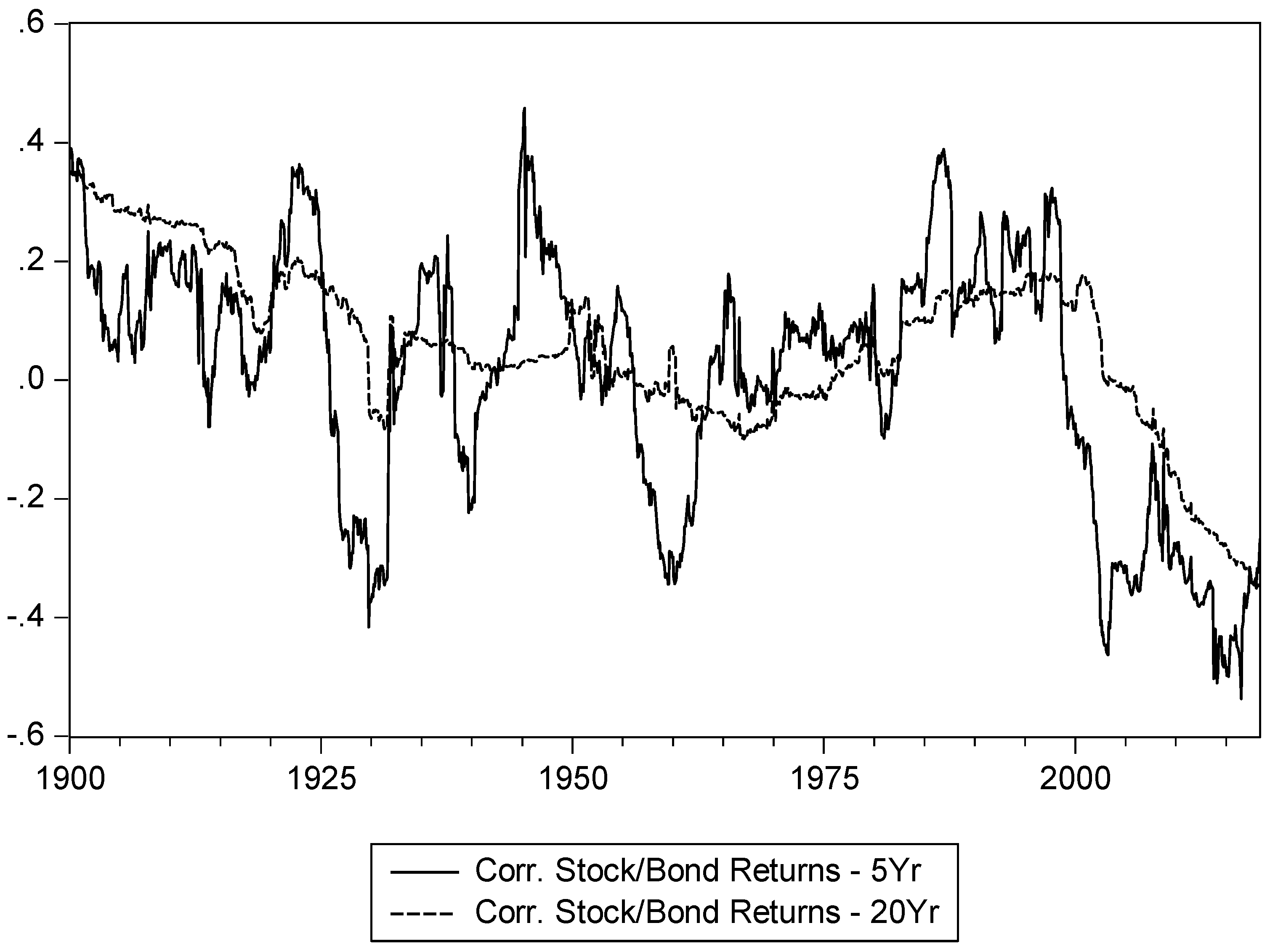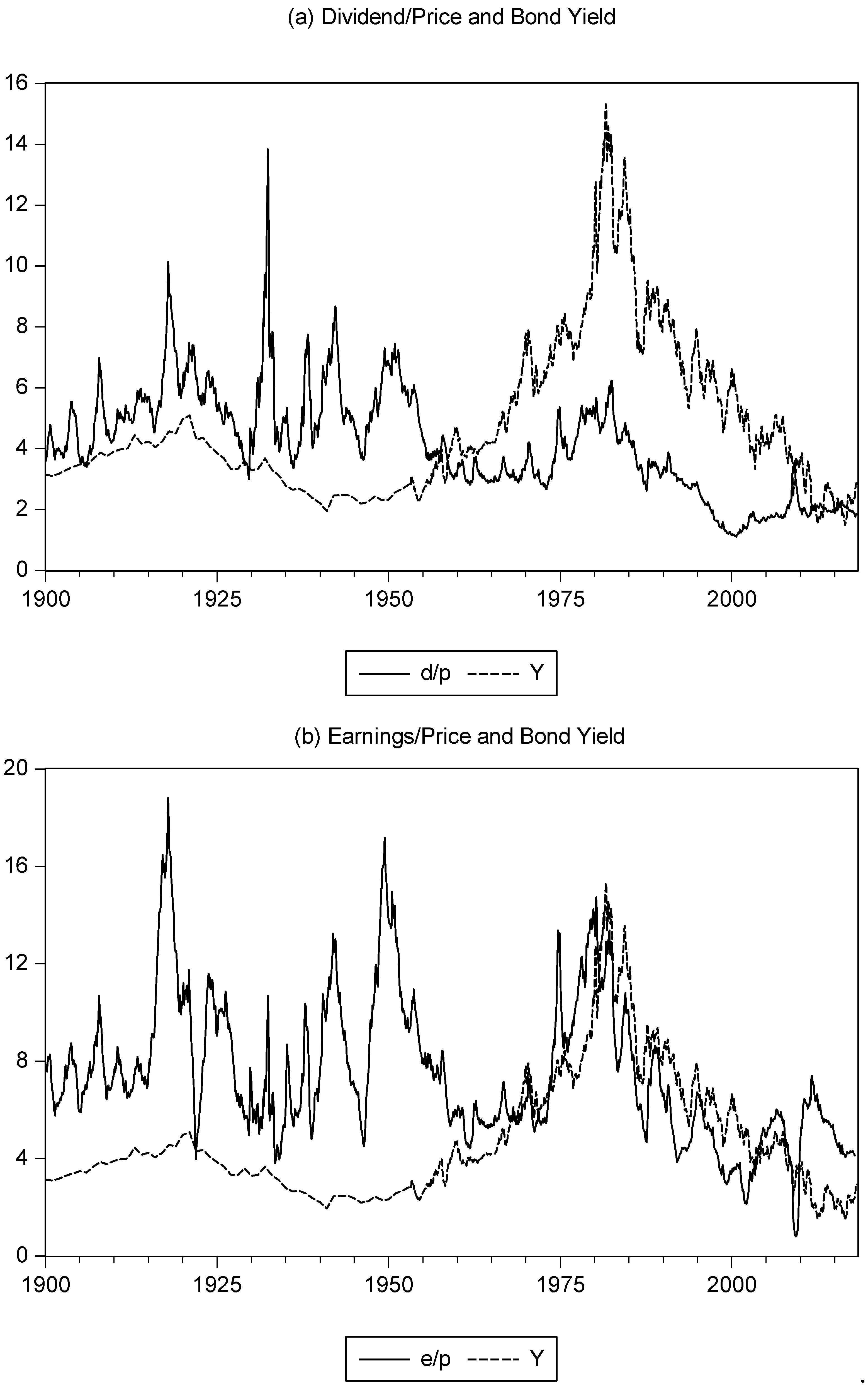To illustrate the nature of the changing relation between stock and bonds, Figure 1 presents the 5-year and 20-year rolling correlations for stock and bond returns, while Figure 2 presents the plots of the equity yield (d/p and e/p) and bond yield, Y.

In Figure 1, we can see that the stock and bond return correlation has switched between periods of positive and negative values. While the overall average value is positive (0.11 for the 5-year moving correlation and 0.06 for the 20-year moving correlation), the correlation turns negative over several extended time periods. Notably, the correlation is negative over the period from the mid-1920s until the early 1930s, from the mid-1950s until the mid-1960s, and from the late 1990s until the end of the sample, with shorter negative periods around the late 1930s/early 1940s and the early 1980s. Each of these periods can be characterised as turbulent events in financial markets, and the wider economy and often includes recessionary periods.

With regard to Figure 2, we observe, similar to Asness (2000), that the equity yield (both d/p and e/p) is greater than the bond yield over the first part of the sample while, from mid-1950, the bond yield is greater than the d/p, and starts to converge with the e/p series (and more obviously during the later 1960s). However, as our sample extends beyond that in Asness (which ends in 1998), we also observe d/p series converging with the bond yield and the e/p series increasing above it during the 2010s (arguably the e/p series began to move above the bond yield during the mid-2000s, but this process was interrupted by the financial crisis). Thus, we see the relation between the equity and bond yield switching in a way that occurred only once before in the sample period and over 50 years ago. Understanding this change is important for enhancing our knowledge of portfolio management and the relation between assets.

Asness argues that the changing nature of the relation between stocks and bonds is largely driven by their relative volatilities and, thus,

Table 1. Equity yield regressions.

	Y	σs,t	σb,t	Adj. R2
Volatility Constructed from GARCH(1,1) Model
d/p	0.248 (5.61)	0.492 (6.89)	−1.449 (−9.82)	0.314
e/p	0.620 (6.58)	0.202 (2.88)	−2.251 (−7.09)	0.201
Volatility Constructed Using 20-Year Rolling Standard Deviation
d/p	0.310 (17.82)	0.906 (12.38)	−1.610 (−13.71)	0.568
e/p	0.702 (11.85)	1.287 (7.43)	−2.239 (−9.76)	0.449

Notes: Entries are coefficient values (and Newey–West t-statistics) from Equations (1) and (2).

presents the regression estimates of the above Equations (1) and (2). The equity and bond yields are given as above, while the stock and bond return volatility (standard deviation) series are based on estimated GARCH(1,1) models. Consistent with the results (and hypothesis) of Asness, we see a positive relation between the equity yield and the bond yield, with the equity yield increasing in stock return volatility and decreasing in bond return volatility. Thus, movements in the equity yield around the bond yield are driven by differences in the relative volatility of the two assets. The volatilities, here, are obtained using a GARCH model for stock and bond returns respectively, whereas Asness used rolling 20-year standard deviations. Thus, for robustness, we replicate this approach in the lower half of Table 1, with consistent results reported.

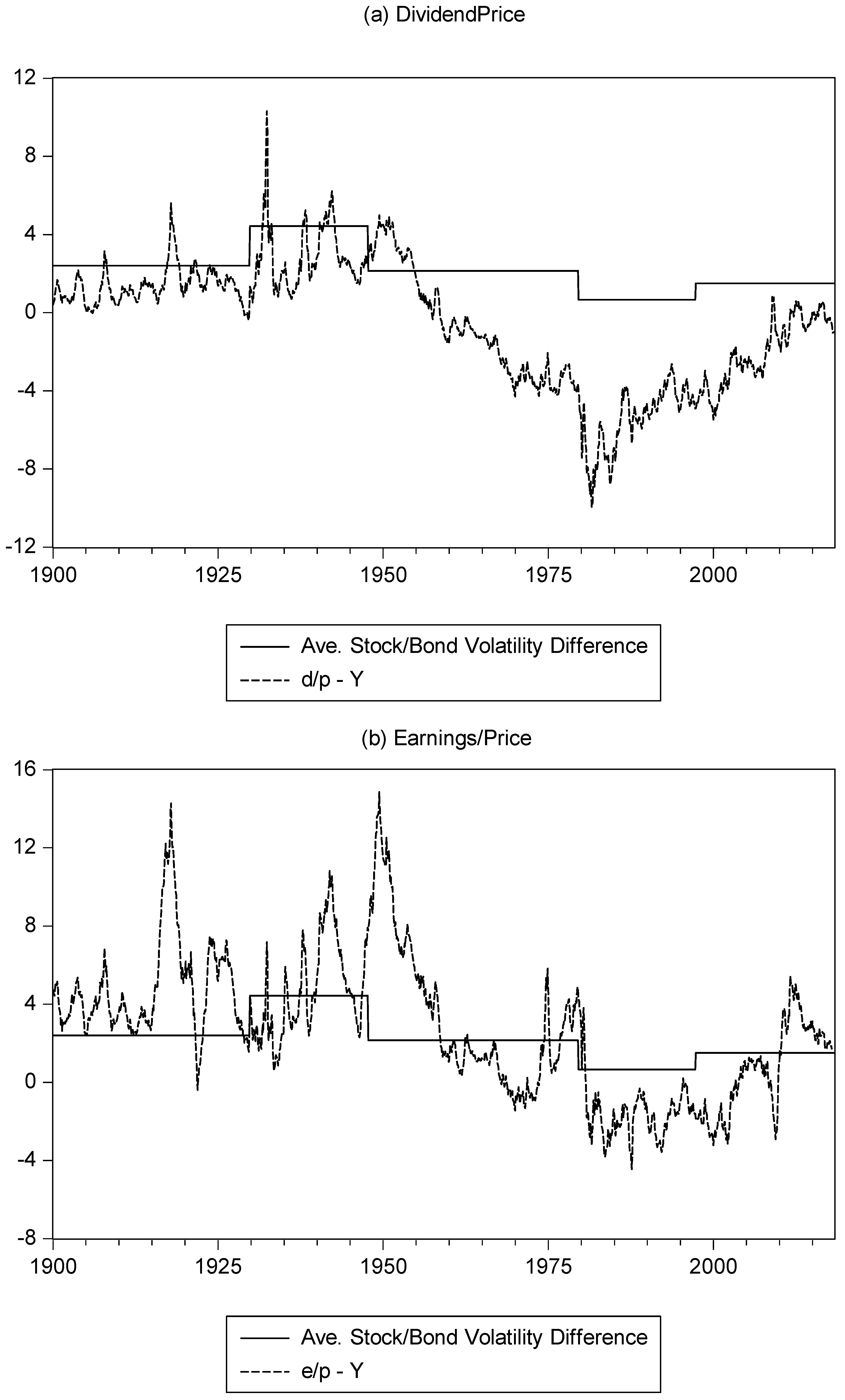
To illustrate how the nature of the equity and bond yields vary with the relative difference in stock and bond volatility, Figure 3 plots the difference between the equity and bond yield, and the difference between the stock and bond return volatilities. To provide clarity in the figure, we obtain the difference between stock return volatility and bond return volatility, and regress this volatility difference series on a constant term. We then use the breakpoint procedure of (Bai and Perron 1998, 2003a, 2003b) to identify periods where there is a break in the constant (the average value of the volatility difference). Figure 3 thus plots this breaking mean difference together with the difference between the d/p and e/p series against the bond yield, respectively. While there is not an exact correspondence between the two series in this figure, it is apparent that a lower volatility difference is consistent with a lower (and negative) yield difference. Equally, the increase in stock return volatility relative to bond return volatility in the late 1990s is consistent with the increase in the equity yield relative to the bond yield seen towards the end of the sample period. In terms of the history of the data, we note from Figure 2 that the equity yield is above the bond yield prior to the mid-1950s. Moreover, this difference increases over the period from 1930 to (approximately) the mid/late1940s. This period is consistent with higher stock return volatility relative to bond return volatility. A fall in this relative volatility position is reflected in the change in the two yields, a position that becomes more extreme during the 1980s and first half of the1990s, as stock volatility falls further relative to bond volatility. The rise in relative stock volatility during the late 1990s is reflected in equity (especially the earnings) yield once again moving higher than bond yields.

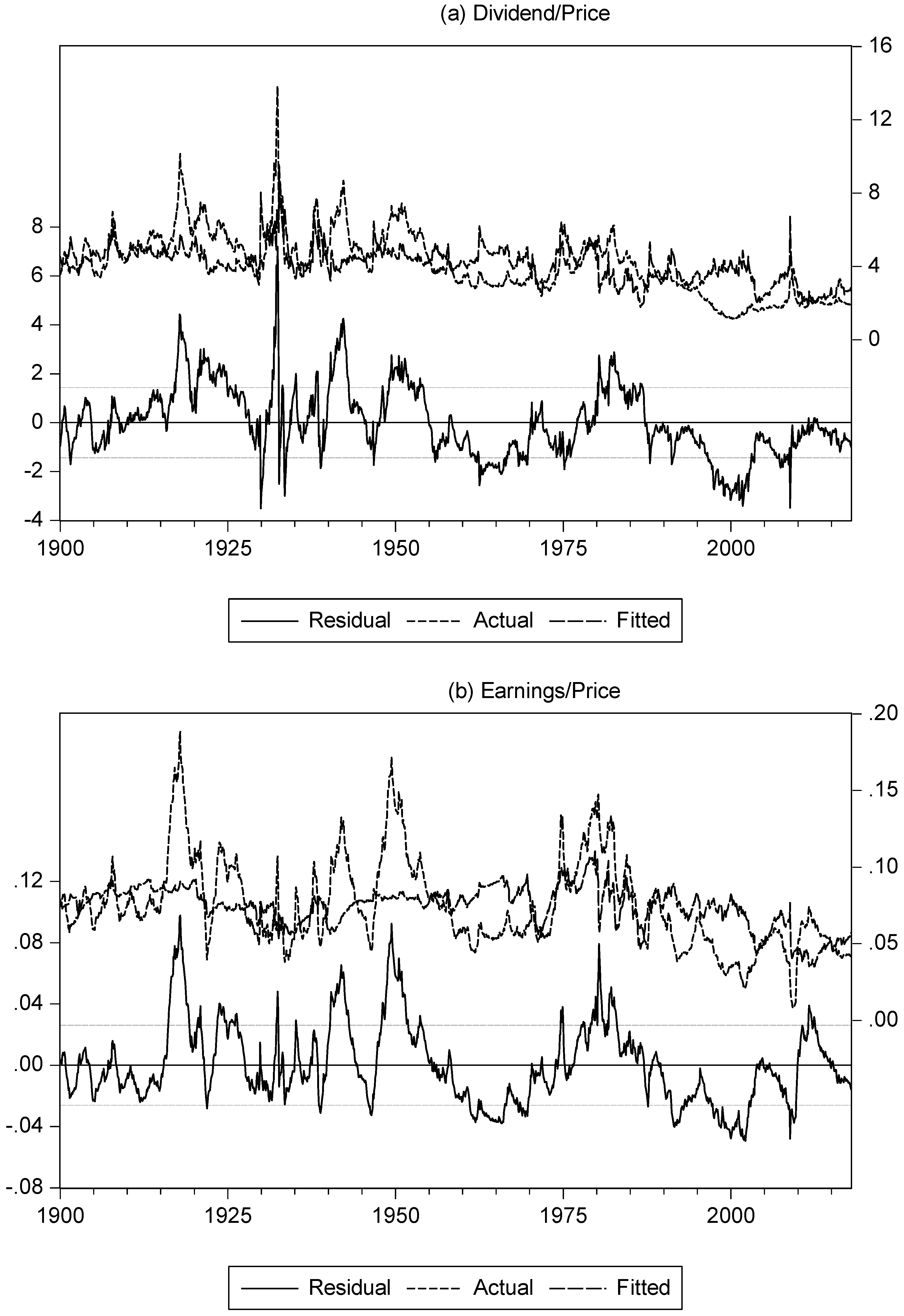
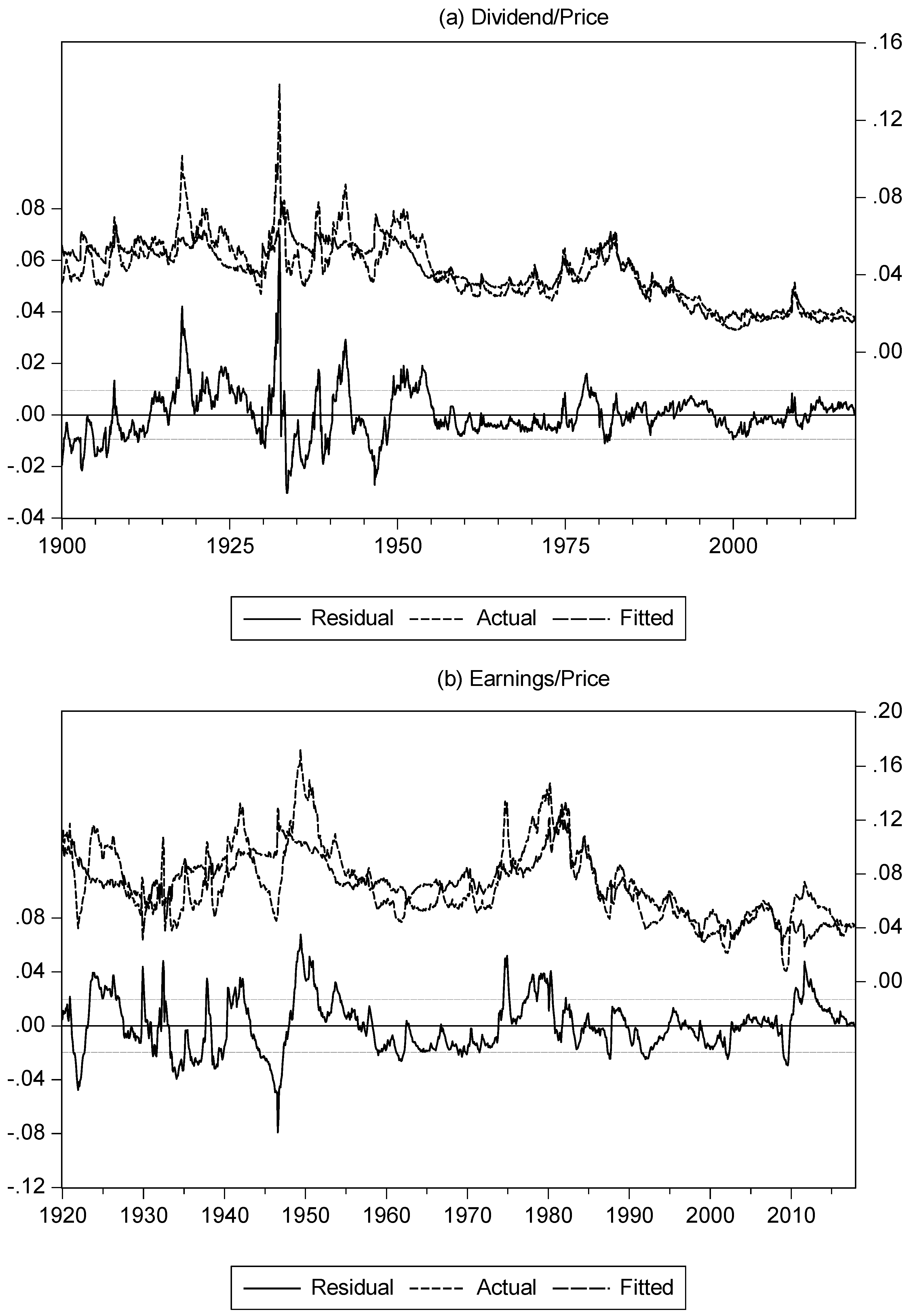
Figure 4 plots the actual and fitted equity yields together with the corresponding residuals, akin to Figure 3 and Figure 4 in (Asness 2000). As with the graphs in Asness, there are periods where the fitted series is above and below the actual series. However, notably, with an interruption from the financial crisis, the model fitted value is above the actual value, almost consistently, from the early/mid 1990s onwards. A similar effect can be seen in Figure 4 of Asness, although the sample period ends in 1998. A similar but shorter period, where the fitted value is noticeably above the actual value, occurs from the late 1950s to 1970. This suggests that while the model largely explains the movement of equity yields, there are periods where the model systematically overestimates the value of the equity yield; this includes for the past 20 years, which is of notable current interest.1

3. Sub-Sample Behaviour

In this section we consider two approaches to examine sub-sample behaviour within the nature of the stock and bond yields relation. First, we consider temporal variation in the above regressions and, second, we examine whether the coefficients change across different values of the dependent variable using a quantile regression approach. The above analysis is conducted over the full sample from 1900 to 2018. However, it is likely that the nature of the relations may evolve over time, indeed Asness (2000) notes some instability in the full period under examination. Such a changing nature of the relation may imply different dynamics for the interaction between stocks and bonds. To examine the nature of the time-variation, we consider two approaches. First, we use the Bai–Perron breakpoint test, with the results reported in

Table 2. Equity yield breakpoint regressions.

	D/P	E/P
Sub-Sample 1	1900:01–1919:04	1900:01–1919:04
Y	2.8224 (9.34)	5.422 (5.20)
σs,t	0.570 (4.86)	0.692 (1.79)
σb,t	3.090 (4.88)	8.575 (3.84)
Sub-Sample 2	1919:05–1937:04	1919:05–1940:01
Y	1.463 (8.32)	1.384 (5.12)
σs,t	0.125 (1.47)	0.066 (0.57)
σb,t	1.187 (1.48)	−2.091 (−2.48)
Sub-Sample 3	1937:05–1954:12	1940:02–1960:12
Y	1.709 (1.98)	−1.797 (−3.79)
σs,t	0.019 (0.15)	0.372 (0.66)
σb,t	1.191 (1.63)	−1.353 (−0.97)
Sub-Sample 4	1955:01–1973:10	1961:01–1989:12
Y	−0.167 (2.45)	1.248 (10.20)
σs,t	0.290 (3.40)	0.497 (2.49)
σb,t	0.152 (1.22)	−2.081 (−5.63)
Sub-Sample 5	1973:11–1996:02	1990:01–2017:12
Y	0.415 (8.65)	0.013 (0.16)
σs,t	0.195 (2.55)	−0.754 (−6.09)
σb,t	−0.595 (−3.27)	1.447 (2.60)
Sub-Sample 6	1996:03–2018:03
Y	−0.138 (−3.57)
σs,t	0.107 (1.70)
σb,t	0.117 (0.96)
Adj. R2	0.827	0.652

Notes: Entries are coefficient values (and Newey–West t-statistics) from Equations (1) and (2) using the breakpoint methodology of Bai–Perron.

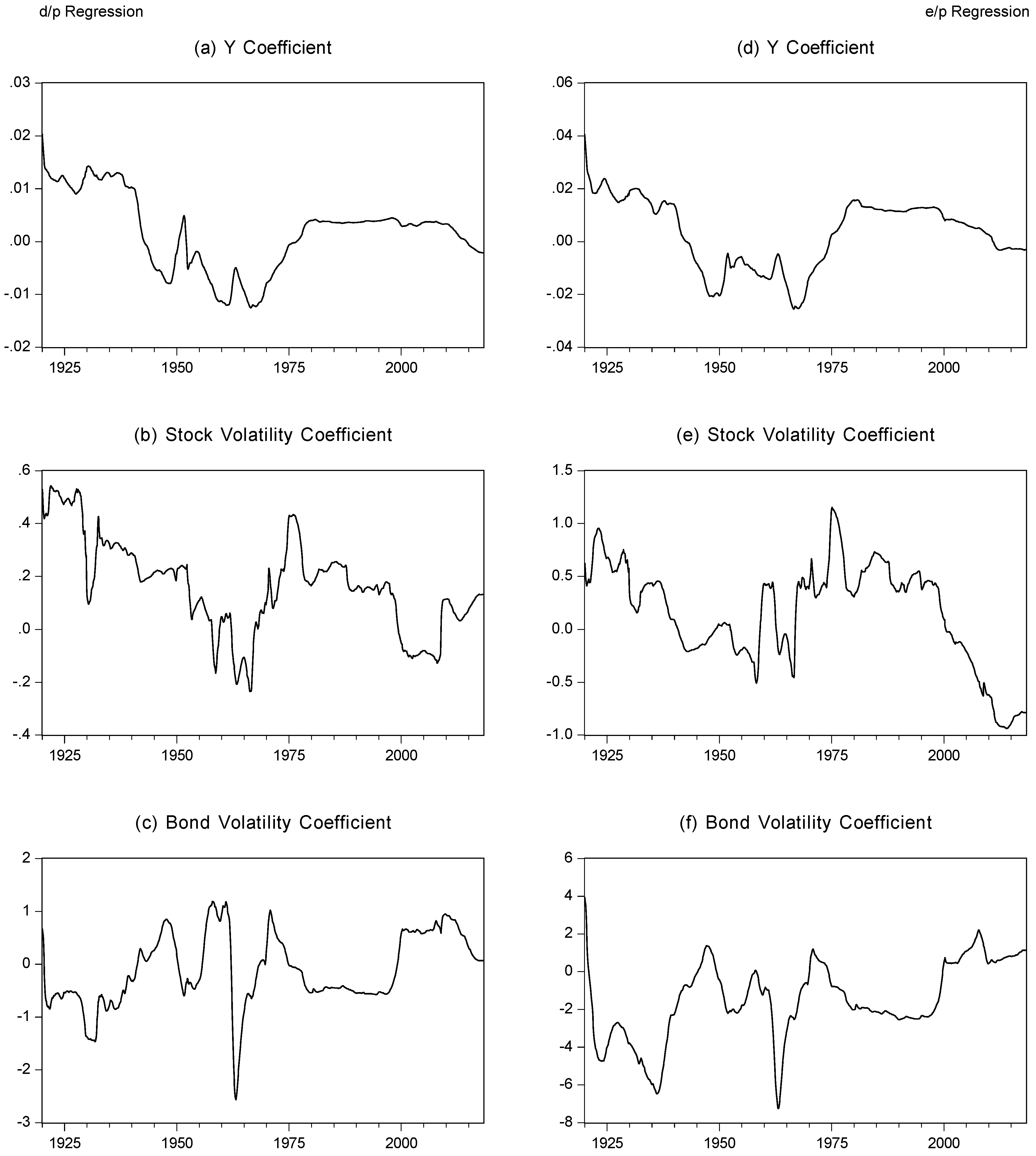
and, second, we use a 20-year rolling regression approach, with the time-varying coefficient values presented in Figure 5.

Examining the results of the Bai–Perron breakpoint regressions, we can see that the sign of the relation between the equity yield and the bond yield is largely positive and significant through the sample period, but there are episodes of a negative relation. Across the d/p and e/p regressions, there are some differences in the timing and number of breaks, but broad similarity in the nature of the relations. In the d/p regression, there is a positive and significant relation with the bond yield from the start of the sample period until the mid-1950s while, for the e/p regression, a positive relation is noted from the start of the sample until 1940, whereupon a negative relation is noted until 1960. For the d/p regression, the negative relation also lasts for 20 years until the mid-1970s. For the e/p regression, the relation is then positive until the end of the sample period, albeit insignificant from 1990. For the d/p regression, the relation again turns negative from 1996 until the end of the sample. The change in the sign of the relation, from positive to negative over the period around the 1950s and 1960s, is consistent with the time period note in Figure 2, as when the behaviour of the equity and bond yields relative values changed. Equally, the negative (d/p regression) or insignificant (e/p regression) coefficient in the last sub-sample period is consistent with the seeming change in the relative values of the equity and bond yields observed in the (approximately) last twenty-year period of the sample.

For the stock and bond return volatility parameters, there is less consistency in the nature and significance of the regression coefficients. For the d/p regression, stock return volatility is positive for the entire sample period, however, it is statistically insignificant (at the 5% level) for much of the sample, only being significant between 1900 to 1919 and 1973 to 1996. The volatility of the bond return is positive and significant between 1900 to 1919, and then positive and statistically insignificant through the rest of the sample period, except between 1973–1996, whereupon it turns negative and significant. For the e/p regression, the volatility of the stock return is positive between 1900–1990 and significantly so from 1961. However, the coefficient turns negative from 1990 onwards. The volatility of the bond return has a positive relation between 1900–1919, and from 1990 until the end of the sample, while exhibiting a negative coefficient between these dates.

Figure 5 presents the rolling regression coefficients for the d/p and e/p regressions, and illustrates a degree of consistency across the two regressions. Moreover, they suggest a significant change in behaviour during the most recent time period. For the bond yield coefficient, as noted above, this is expected to be positive; in both the d/p and e/p regressions, we can observe notable periods where the coefficient turns negative, this is particularly true of the period between the early 1940s until the mid-1970s, and during the 2010s until the end of the sample period. For the stock return volatility, again, this coefficient is expected to be positive, but is negative for the d/p series from the late 1950s to late 1960s, and the late 1990s to the late 2000s. For the e/p regression, there is slightly greater evidence of a negative relation, running from the early 1940s to the mid-1960s and from the early 2000s until the end of the sample. The coefficient on bond return volatility is expected to be negative, while the rolling coefficients reveal notable periods where it is positive. Across both regressions, this can be seen in the period from the early 1940s to early 1950s, the mid-1950s to early 1960s, the early to mid-1970s, and from the late 1990s until the end of the sample period.

The two procedures, here, suggest notable time-variation in the nature of the relation between the equity yield and the bond yield, and stock and bond volatilities. Following the model of Asness (2000), we expect to observe a positive relation between the two yields, with the equity yield increasing in rising stock volatility and falling bond volatility. The evidence above suggests that this broad relation holds for much of our sample period, notably, over much of the pre-second world war period, and between the mid-1970s until the end of the 1990s. However, of notable pertinence, since the beginning of the 2000s, and especially since the beginning of the 2010s, the nature of the relations has been reversed. Similar periods where the coefficients signs were reversed can be seen in the late 1940s and late 1950s. Thus, the shift between the relative position of equity and bond yields observed during the sample period can be characterised by a change in regression coefficients. A similar change can be observed in the current data, and may indicate a further change in the relative equity and bond yields.

An alternative approach to examining variation within the coefficients is through a quantile regression approach. A quantile regression models the quantiles (partitions or subsets) of the dependent variable given the explanatory variables (Koenker and Bassett 1978; Koenker and Hallock 2001). The quantile regression therefore extends the linear models in Equations (1) and (2) by allowing a different coefficient for each specified quantile:

(d(e)/p)_t = α^(q) + β^(q) Y_t + γ^(q) σ_s,t + λ^(q) σ_b,t + ε_t,

(3)

where α^(q) represents the constant term for each estimated quantile (q); β^(q), γ^(q), and λ^(q) are the slope coefficients that reveal the relation at each quantile; and, again, ε_t is the error term.

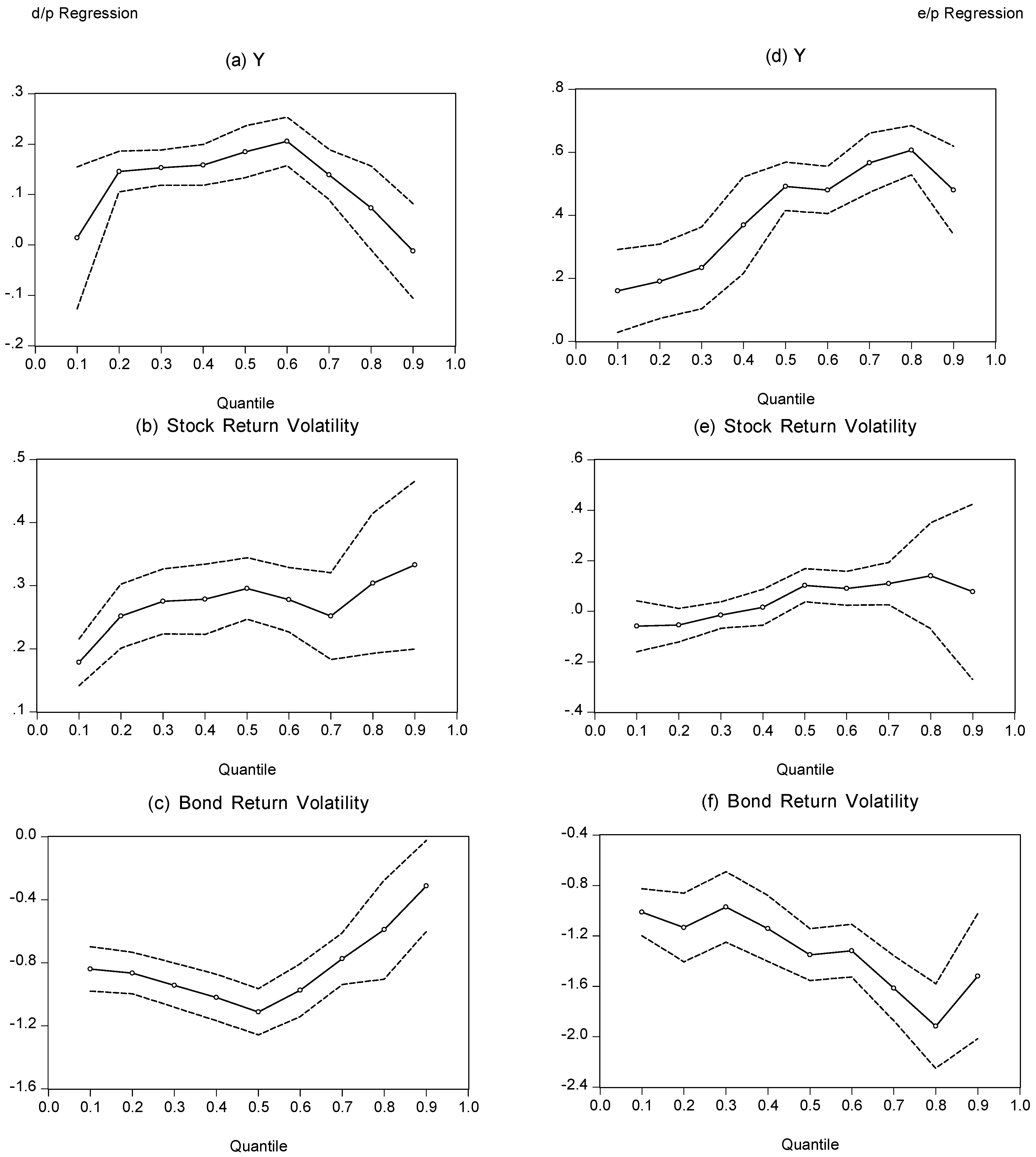
Figure 6 presents the quantile regression coefficients. Of notable interest is whether the strength of the relation between the dependent and explanatory variables changes in a systematic way. For the d/p series, we can see that the coefficient on the bond yield series is broadly consistent in value across most of the quantiles but, at the low and high extremes, differs in value. For most of the quantiles, the coefficient on the bond yield is positive, statistically significant, and in the range of between approximately 0.15 and 0.20. By contrast, at low and high values of the d/p series, the coefficient becomes statistically insignificant and even negative at the highest quantile. For the two volatility series, the respective coefficients maintain the same sign (positive for stock volatility and negative for bond volatility) and are statistically significant throughout. Notwithstanding this, we can see that, for stock return volatility, the coefficient increases in magnitude, while, for the bond return volatility series, it decreases in magnitude across different values of the d/p series.

The quantile graphs for the e/p regression are broadly similar to those of the d/p regression, but do exhibit some notable differences. The coefficient on the bond yield variable is positive and significant, although now throughout all the quantiles, including the extreme values as opposed to those observed for the d/p regression. For the stock return volatility, again, the coefficient is broadly positive and significant, although at the lower end of the e/p scale, and the coefficients are negative and statistically insignificant. The coefficients for the bond return volatility series are negative and statistically significant, although we now observe the strength of the relation increasing with the value of e/p, as opposed to the d/p regression, where the strength of the relation declines over larger values of the dependent variable. Thus, the sign and significance of the coefficients in the d/p and e/p regressions are broadly consistent, but we do observe some differences in the nature of the pattern across different quantiles.

4. Extending the Model

The above analysis suggests that movement in stock market valuations are linked to movements in bond yields and the relative values of stock and bond return volatility. However, the evidence equally suggests that the nature of these relations varies over time, with periods where equity and bond yields are moving in opposite directions, and where the effect of stock and bond volatility reversed from their expected direction.

Given this, we seek to examine the nature of the relations further, in a desire to understand the drivers of equity yield movements and stock and bond interaction. Asness (2000) uses a 20-year rolling average measure in constructing volatility measures, and argues this essentially represents a generation. As such, movements in the equity yield and its relation with the bond yield reflect investors’ experience of recent asset price movements. Supporting this view, we seek to extend the above model by separating volatility into a (long-run) moving average component, and a (short-run) deviation from the average component.

Table 3. Equity yield regressions separating volatility.

	Y	σs,t-LR	σb,t-LR	σs,t-SR	σb,t-SR	Adj. R2
d/p	0.252 (9.83)	1.407 (10.75)	−1.946 (−14.88)	0.262 (3.70)	−0.199 (−2.62)	0.582
e/p	0.672 (8.01)	1.813 (6.24)	−2.854 (−8.97)	−0.128 (−2.48)	−0.607 (−3.62)	0.415

Notes: Entries are coefficient values (and Newey–West t-statistics) from Equations (1) and (2). Volatility is separated into a long-run component given by a 20-year moving average, and a short-run component as the deviation from this average.

presents the results in which the stock and bond return volatilities, obtained from a GARCH(1,1) model, are separated into a long-run component given by a 20-year moving average, and a short-run component given by the deviations of volatility from this 20-year moving average. Thus, we are suggesting that the effect on the equity yield of volatility impacts over differing time-horizons. The results continue to support a positive relation between the equity yield and the bond yield and, equally, a positive relation with (long-run) stock return volatility and a negative relation with (long-run) bond volatility. However, there is some discrepancy in the short-run behaviour with stock volatility having a positive impact on the d/p regression, but a negative impact on the e/p regression. For both regressions, short-run bond volatility has a negative relation. This difference in respect of short-run stock volatility may arise as firms manage dividends to ensure an increase in the equity yield in the face of higher volatility, in contrast to more variable movement in earnings.

Continuing the line of thought that it is recent experience affects the behaviour of the equity yield, and we argue that it is not only the volatility of stock and bonds that matter in terms of altering investor perceptions of risk, but also macroeconomic conditions more generally. Inflation exhibited a higher degree of volatility from the beginning of the sample period until the mid-1950s, after which volatility declined. The standard deviation of annualised and monthly inflation, from the beginning of the sample until the end of 1954, is 6.63% and 1.07%, respectively. From 1955 to the end of the sample, the equivalent values are 2.68% and 0.35%, respectively. This change in the behaviour of inflation may help explain the change in the relation between equity and bond yields observed in Figure 2. Most recently, we have observed a period of very tranquil inflation, which has been followed by a noticeable uptick in inflation volatility. While this increase in inflation volatility by long-run historical standards may seem relatively mild, it is noticeable when only examining recent history. Over the 1990s period, the standard deviation for annual and monthly inflation is 1.08% and 0.19% respectively, while, over the 2000s, it is 1.27% and 0.38%. For current investors, the higher historical inflation volatility (even that observed during the 1970s) is unlikely to impact current decisions. By contrast, the recent increase in inflation volatility may cause investors to raise their expectations of future risk.

Table 4. Equity yield regressions with inflation and separating volatility.

	Y	σs,t-LR	σb,t-LR	σI,t-LR	σs,t-SR	σb,t-SR	σI,t-SR	R2
d/p	0.272 (11.48)	1.375 (10.42)	−1.145 (−10.84)	1.652 (9.36)	0.166 (2.47)	0.037 (0.28)	0.694 (2.37)	0.700
e/p	0.642 (8.31)	1.692 (2.19)	−1.986 (−6.36)	1.860 (2.72)	−0.311 (3.27)	−0.268 (−0.79)	1.619 (2.19)	0.525

Notes: Entries are coefficient values (and Newey–West t-statistics) from Equations (1) and (2), but with inflation (first-difference of monthly CPI) added. Volatility is separated into a long-run component given by a 20-year moving average and a short-run component as the deviation from this average.

presents the results of the model that now includes inflation volatility. As with stock and bond return volatility, this series is obtained from a GARCH(1,1) model for monthly changes in the CPI (Consumer Price Index), and then using a 20-year moving average to separate long- and short-run effects. The results, for the variables previously considered in Table 3, continue to hold in terms of coefficient sign and statistical significance. Thus, we observe a positive relation between the equity yield and the bond yield and long-run stock volatility, and a negative relation between the equity yield and long-run bond volatility. A negative relation also exists with short-run bond volatility, while short-run stock volatility differs between the d/p regression (positive) and the e/p regression (negative). Inflation has a positive effect of the equity yield both in the long-run and the short-run. Moreover, the relation, which is statistically significant, has a larger coefficient than for stock return volatility and, while that difference may be more marginal in the long-run, it is noticeable in the short-run. These results support the view that changes in inflation affect investor outlook for equities and the equity yield. Notably, the switch in the relative position of equity and bond yield during the second half of the 1900s occurred when inflation volatility substantially declined. The potential switch back, occurring in the 2000s, may arise as inflation volatility increases again (in comparison to recent history).

A further point of note is that the results in Table 3 and Table 4 show a noticeable improvement in model fit over the results reported in Table 1. The adjusted R² increases from approximately 0.3 and 0.2 for the d/p and e/p regressions, respectively, to 0.6 and 0.4 in Table 3, and to 0.7 and 0.5 in Table 4. To further illustrate the improvement in fit, Figure 7 presents the actual, fitted, and residual values, equivalent of Figure 4 for the original model. In comparison to the earlier model, we can see that by including inflation, the large discrepancies between the fitted and actual values that occurred in the 1960s, and from the late 1990s until the end of the sample, no longer occur. This supports the extended model in providing a better understanding of equity yield movement.

Robustness

One potential issue arising from the above analysis and an examination of Figure 4 and Figure 7 is the apparent residual serial correlation that remains. While such residual serial correlation implies inefficient estimation and, thus, bias in the standard errors and t-statistics only, and not the coefficient values, it does imply the potential for omitted variables to exist that will further enhance the model. Indeed, the R² values of approximately 0.70 for the d/p regression and 0.50 for the e/p regression suggest room for improvement.

While we leave the finding of such variables for further research, it still leaves the question of whether we can account for the residual serial correlation within our model, and whether that affects the nature of the reported results. Therefore, we consider lags of the dependent variable in order to eliminate the residual serial correlation. We select the lag length both on the basis of residual tests and information criteria. The resulting number of lags is selected as two for the d/p regression and four for the e/p regression, with the results reported in

Table 5. Equity yield regressions with inflation, separating volatility, and lags of the dependent variable.

	Y	σs,t-LR	σb,t-LR	σI,t-LR	σs,t-SR	σb,t-SR	σI,t-SR	Lags	R2
d/p	0.151 (2.17)	0.755 (1.99)	−0.962 (−2.29)	0.845 (2.63)	0.055 (1.96)	0.017 (1.13)	0.563 (2.467)	0.954 [0.00]	0.981
e/p	0.477 (2.98)	0.423 (2.61)	−0.575 (−2.38)	0.486 (2.05)	−0.251 (−3.93)	−0.412 (−0.18)	0.477 (2.57)	0.974 [0.00]	0.987

Notes: Entries are coefficient values (and Newey–West t-statistics) from Equations (1) and (2), but with inflation (first-difference of monthly CPI) added. Volatility is separated into a long-run component given by a 20-year moving average and a short-run component as the deviation from this average. Lags refers to the sum of the autoregressive parameters with the number in square brackets the p-value of a joint significance test.

. Here, we can observe that the key nature of the coefficients in terms of their sign and significance remains. Although, we can note that both the coefficient magnitudes and the strength of statistical significance is lower. In terms of the autoregressive coefficients, we can see a high degree of persistence, with the lags highly statistically significant. The inclusion of the lag terms also noticeably increases the R² values. Overall, the key inference of the results remains the same with the inclusion of the autoregressive lags, and it remains an avenue for future research to see if there are additional explanatory variables to explain the movement of the equity yield, as opposed to using lags of the dependent variable.

5. International Evidence

To provide further robustness to the above results that are obtained for the US, we consider three other major industrialised markets, namely Germany, Japan and the UK. For these markets we have a shorter span of data ranging from the start of 1980 for Germany and the UK and 1990 for Japan. For each of these markets, we obtain data on the d/p and e/p series, a 10-year Treasury bond and stock and bond returns. All the data in this section is obtained from DataStream and based on the total market index. In order to improve the accuracy of the results, we obtain daily values of the stock and bond index series and construct monthly volatilities based on aggregating daily squared returns. We also obtain CPI data, which is only available monthly and thus again use a GARCH(1,1) model to obtain volatility.

The results of estimating the extended model are reported in

Table 6. Equity yield regressions with inflation and separating volatility–additional markets.

	Y	σs,t-LR	σb,t-LR	σI,t-LR	σs,t-SR	σb,t-SR	σI,t-SR	Adj. R2
Germany
d/p	0.158 (4.81)	0.923 (8.88)	4.315 (2.09)	3.237 (1.98)	0.202 (2.72)	0.310 (1.09)	0.913 (1.70)	0.614
e/p	−0.153 (−0.15)	1.849 (5.84)	1.141 (2.57)	2.085 (4.99)	0.328 (1.83)	0.958 (1.89)	1.155 (1.08)	0.543
Japan
d/p	0.294 (0.63)	0.698 (5.47)	−1.339 (−2.95)	3.939 (1.43)	0.068 (2.42)	0.014 (2.06)	0.152 (2.59)	0.836
e/p	−0.237 (−0.11)	1.216 (3.24)	−3.257 (−4.81)	3.168 (3.16)	0.103 (1.80)	0.688 (1.39)	0.629 (3.87)	0.850
UK
d/p	0.244 (5.83)	4.805 (3.27)	4.405 (3.51)	1.557 (2.37)	0.454 (4.46)	1.724 (0.77)	0.954 (2.02)	0.696
e/p	0.508 (4.93)	0.290 (7.01)	−1.215 (−3.55)	2.730 (2.22)	0.710 (2.79)	0.523 (0.91)	1.313 (0.50)	0.680

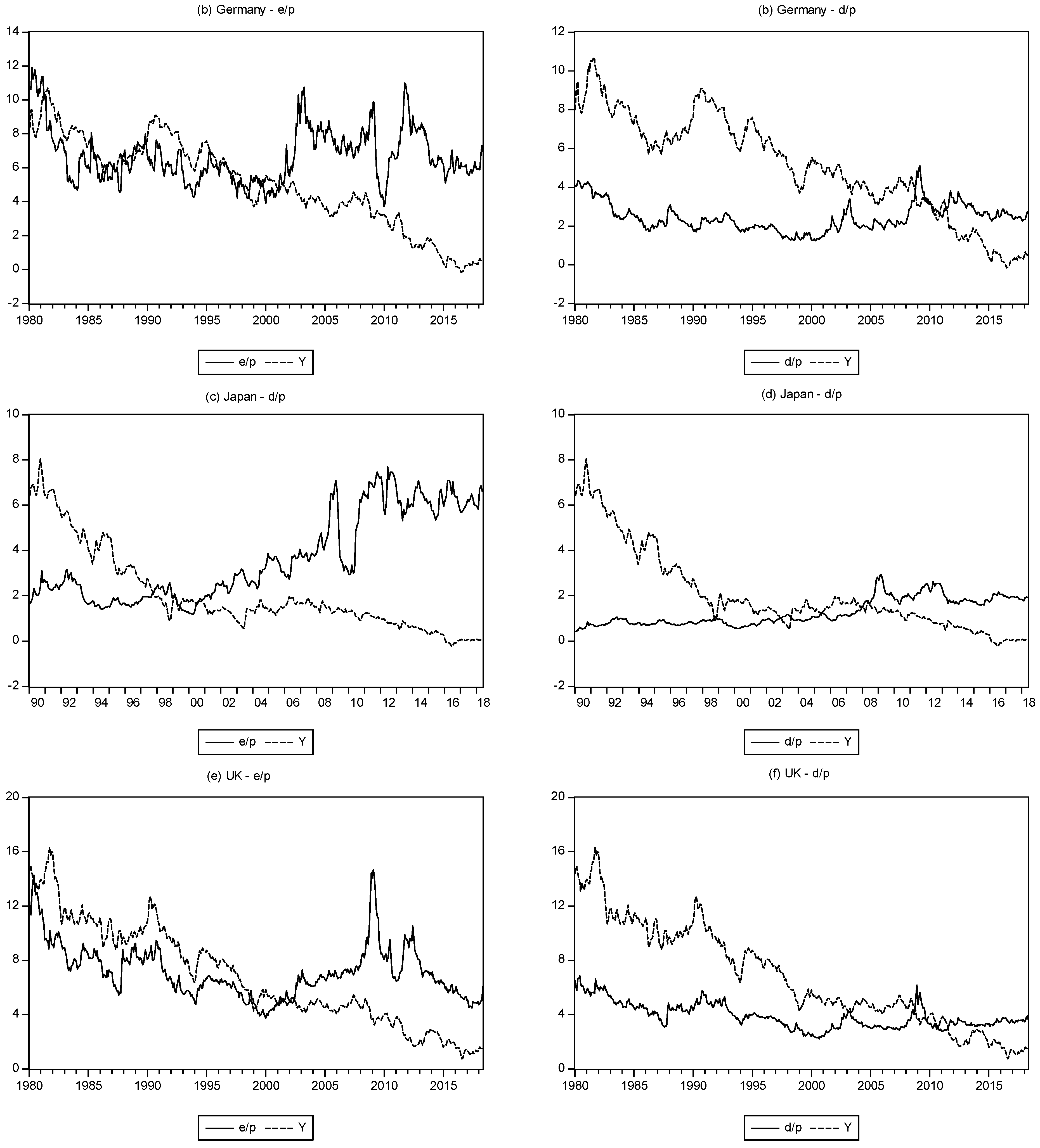
Notes: Entries are coefficient values (and Newey–West t-statistics) from Equations (1) and (2), but with inflation (first-difference of monthly CPI) added. Volatility is separated into a long-run component given by a 10-year moving average and a short-run component as the deviation from this average.

, where we again separate the volatility series in to long- and short-run component, although now we use a 10-year moving average as the available data sample is shorter. Prior to estimating the models, Figure 8 plots the equity and bond yields for each market. As with the US data, again we can observe a crossover point with the bond yield higher at the start of the sample period and the equity yield higher at the end of the sample period. We can also observe that the change point occurs later in the sample for the d/p yield series compared to the e/p yield.

Examining the estimated results, we observe that the same general pattern of results as found for the United States broadly holds, noting that we are comparing not with the full US sample, but with the results obtained only in the latter part of the sample. Specifically, we can see that the nature of the results for the equity yield and bond yield are mixed. A positive relation between the d/p series and the bond yield exists for all markets, while a positive relation also for the e/p and bond yield series for the United Kingdom. By contrast, a negative relation holds with the e/p series for Germany and Japan, although the coefficient is not statistically significance (indeed for Japan, the equivalent coefficient in the d/p regression is also insignificant). The equity yield exhibits a positive relation with long-run stock return volatility for all series, while the relation with long-run bond return volatility is mixed, positive for Germany and in the d/p regression for the United Kingdom, and negative for Japan and the e/p regression for the United Kingdom. For all series, the short-run volatility components indicate a positive relation with the equity yield. Pertinent for our analysis, however, is that we see that both long-run and short-run inflation has a positive influence on the equity yield for all three markets, although there some short-run components are not statistically significant.

Thus, these international results confirm two observations from the US analysis. First, over the most recent period, the nature of the equity and bond yield and the stock and bond volatility variables, no longer exhibits a consistent relation. Notably, the relative values of the equity and bond yields appear to switch during the sample. Second, inflation plays a key role in the movement of equity yields, and long-run inflation exhibits a consistent relation, supporting the view that it plays a pivotal role in the dynamics of the equity yield.

6. Summary and Conclusions

This paper examines the behaviour of the equity yield with respect to the bond yield, and uses the relative volatility of stock and bond returns, as suggested in Asness (2000), to explain the movements of the yields. Using data for the United States over the period from 1900 to 2018, we observe, as previously reported, a switch in the relative values of the equity and bond yields, with the former exhibiting a larger value until the mid-1900s, and the latter exhibiting the larger value subsequently. Our evidence supports the view that this switch occurred as stock return volatility fell relative to bond return volatility.

However, in extending the dataset, we reveal that, over the 2000s, the equity yield once again becomes larger than the bond yield, and this occurs at a point when stock return volatility increases relative to bond return volatility. Moreover, using breakpoint and rolling regressions, we show noticeable variation in the coefficients between the equity yield and the bond yield and the two volatility series. Notably, we see a switch in the coefficient values, with the bond yield and stock return volatility coefficients becoming negative, and the bond volatility coefficient becoming positive, at the time when the relative positions of the equity and bond yields switch.

In seeking to understand the behaviour of the equity yield and the switching behaviour with respect to the bond yield, we also consider the role of inflation. Over the period from 1900 to the mid-1900s, inflation was highly volatile, and this is a period when the equity yield was greater than the bond yield. Subsequently, inflation volatility fell, and the value of the bond yield increased to be higher than the equity yield. Equally, we observe an increase in inflation volatility during the 2000s, and while this increase is small in terms of the full history of data, it is noticeable compared to the recent, tranquil, past. Thus, higher inflation volatility (relative to its recent history) is consistent with an increase in the equity yield. Having established this result using a long span of US data, we repeat the exercise using a shorter data period for Germany, Japan, and the United Kingdom. The results reveal that the relation between the equity yield, bond yield, stock return, and bond return volatility is mixed, as it is with the US data. However, consistent evidence of inflation volatility affecting the equity yield is revealed.

Understanding the behaviour of the equity yield and its relation to the bond yield remain important for portfolio managers and those engaged in modelling the interaction between asset classes. During the mid-1900s, the equity yield, which was previously greater than the bond yield, declined while the bond yield rose and became higher. In seeking to understand this, it is put forward that the role of stock and bond return volatility is key. Evidence from the 2000s suggests that the relative values of the equity and bond yield may have flipped again, with the former now greater. Empirical evidence also suggests that during such periods, the hypothesised relation between the equity yield and the bond yield and the two volatilities equally flips with the expected signs reversing. This paper argues that the relative equity and bond yield values are also driven by inflation volatility. High volatility persisted during the first half of the twentieth century when the equity yield was higher. This was followed by more benign inflation volatility when the bond yield became higher. Evidence reported here suggests that the rise in the equity yield is accompanied by an uptick in inflation volatility relative to its recent tranquillity.