Abstract
The CKLS process (introduced by Chan, Karolyi, Longstaff, and Sanders) is a typical example of a mean-reverting process. It combines random fluctuations with an elastic attraction force that tends to restore the process to a central value. As such, it is widely used to model the stochastic behaviour of various financial assets. However, the calibration of CKLS processes can be problematic, resulting in high levels of uncertainty on the parameter estimates. In this paper we show that it is still possible to draw solid conclusions about certain qualitative aspects of the time series, as the corresponding indicators are relatively insensitive to changes in the CKLS parameters.
1. Introduction and Problem Statement
1.1. Introduction and Motivation
Stochastic processes are widely used to model the fluctuating prices of economic and financial assets. As a consequence, there is a wide range of processes that have been designed to capture various aspects of stochastic behaviour. Within this broad spectrum, the CKLS process (introduced by Chan, Karolyi, Longstaff, and Sanders in Chan et al. (1992)) is a typical example of a mean-reverting process that combines random fluctuations with an elastic attraction force. As a consequence, it tends to restore the process to some central target value after random excursions.
In more detail, the CKLS process describes the behaviour of a positive random variable (; typically measuring daily returns of some financial asset), the dynamics of which is determined by the following stochastic differential equation (SDE) with respect to standard Brownian motion ()
or equivalently,
By comparing these two representations we see that: and conversely , . The reformulation of the SDE in Equation (2) elucidates the meaning of the parameters:
- is the long-term equilibrium value about which the process performs random excursions;
- represents the elastic spring constant that determines how fast random excursions will revert back to the central attractor (a). Large values for k imply a tightly bound process resulting in short excursions;
- is the (specific) volatility;
- measures the sensitivity of the volatility with respect to the current process value.
The reformulation in Equation (2) also makes it clear that k and a model independent qualitative aspects of the process.
The CKLS process has been applied to the modelling of economic assets that tend to vary about some pre-defined set point, such as interest rates or oil price Bu et al. (2010); Croghan et al. (2017). In order to be applied in data analysis, the CKLS process must be calibrated, i.e., the relevant process parameters must be estimated from actually observed time series Dell’Aquila et al. (2003); Salisu and Oloko (2015). This turns out to be a difficult problem, as the information that can be gleaned from individual sample paths is often insufficiently informative to accurately pin down the parameter values. As a consequence, the amount of uncertainty regarding the actual parameter values is often considerable.
1.2. Problem Statement
However, for many applications, the parameters themselves are not the object of interest. Rather, we use these parameters to forecast or explore specific aspects of the data. The aim of this paper is therefore to examine to what extent specific but relevant questions are sensitive to the uncertainties in the parameter estimation. In particular, we investigate the extent to which unusual changes in the WTI oil price and the US interest rate can be explained within the CKLS framework, or whether they are so unlikely that they point to exogenous influences.
To shed light onto the above questions, we quantified the observed erratic behaviour using locally defined features to capture unusual behaviour in the data, such as prolonged up- or down-swings. To this end, we took our inspiration from several recent papers that showed how wavelet analysis can be applied to investigate perturbations in financial time series, e.g., Chatzikonstanti (2017); Dewandaru et al. (2017); Grané and Veiga (2010); Martín-Barragán et al. (2015); Zhou et al. (2018). In particular, a simple but frequently used wavelet is the Haar wavelet which basically computes the first derivative of the signal after averaging at different scales (see left panel of Figure 1 Section 4.1.1). We adopted a similar approach but, for reasons of computational convenience, opted for a smoothed version of the Haar wavelet. More precisely, we used the first derivative () of a Gaussian smoothing kernel of width r:

Figure 1.
Left: The Haar wavelet high-pass convulution filter (of width ). At each point, this convolution filter computed the difference between the 10-point averages on the right and left of the central point. So, in this sense, it is similar to a derivative, except that we compared averages, rather than point values; Right: Example of convolution filter (Gaussian smoothed first derivative). In this case, the filter has a radius of . The filter can be interpreted as a smoothed version of the the Haar wavelet on the left. Since scaled this filter (i.e., varying r) to elicit the response at different scales, this type of filtering is akin to (Haar) wavelet analysis.
This filter (depicted in the right panel of Figure 1 Section 4.1.1) produces a maximal response at positions where the data locally resemble the filter shape, i.e., have up- or down-swings of size r.
1.3. Overview of the Methodology
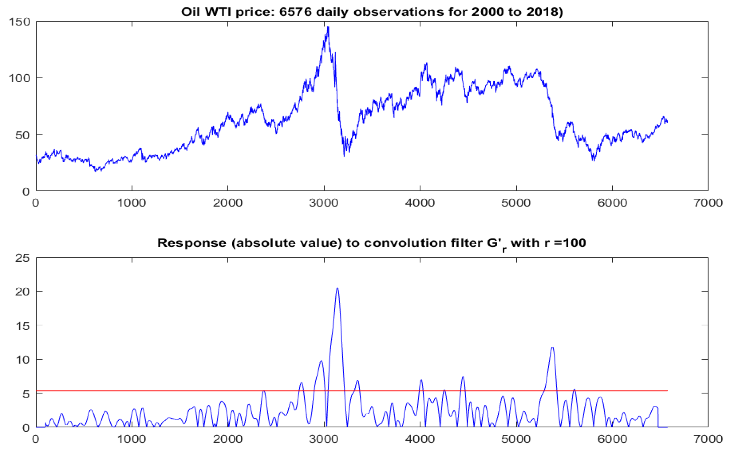
We are now in a position to present the different steps used to address the above question. For the sake of clarity, we illustrate the procedure using the oil price data in Figure 2 in Section 4.1.1 (top panel).
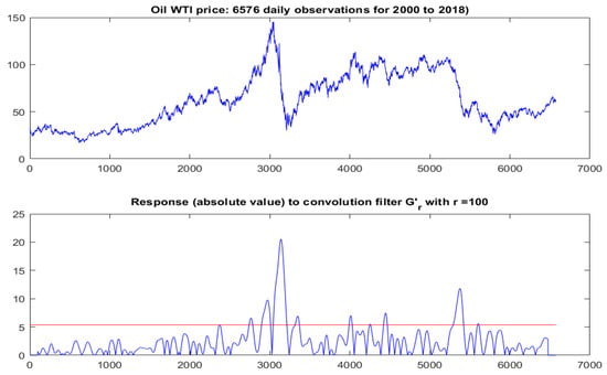
Figure 2.
Top: Oil price data: 6576 daily observations for the period 2000–2018; Bottom: Response (defined in Equation (4)) after convolution with the smoothed first derivative (). As expected, there was a clear peak corresponding to sharp downturn around observation 3000. The size of this peak was measured relative to the 90&-percentile of the response (indicated by the red line), yielding an observed value of (see also Equation (5)).
- We were interested in finding out whether the down-swing around observation 3000 (which corresponds to a period in 2008–2009) is unusual. Since this period comprises 100–200 daily observations, we picked a convolution filter () of size .
- The response (in absolute value) of the original data after convolution with is shown in the bottom panel of Figure 2 in Section 4.1.1. Clearly the most vigorous response occurred around location 3000. However, in and of itself this does not prove anything. The question is whether this response is unusually high.
- To proceed, we first defined a single number to express the size of the maximum response relative to a statistically stable response measure, e.g., the 90%-percentile of the response values (indicated by the red line in the bottom panel of Figure 2 in Section 4.1.1). We denoted the resulting value by , which, for the oil data, turns out to be 3.82.
- Next, we needed to decide whether this observed value for T is exceptional. We assumed that the dynamics underlying the observed time series were indeed governed by a CKLS process, estimated its parameters from the observed data sequence and used the results to generate a large number of simulated sample paths. For each of these simulated sample paths, we computed the corresponding T statistic. This allowed us to estimate the p-value of under the assumption of CKLS dynamics.
- Finally, since we know that the estimated CKLS parameters used to generate sample paths are subject to a considerable amount of uncertainty, we repeated the simulation experiments for a range of likely parameter values. This told us how sensitive our conclusions were to changes in the parameter values, and whether they would hold up if the parameters had slightly different values.
The remainder of this paper is organised as follows. In Section 2 we provide some background on the data that we investigated in the use cases. Section 3 briefly reviews the relevant results reported in the literature. Section 4 tackles, in more detail, the two use cases that were announced in the introduction, and we drew some conclusions in Section 5.
2. Data
In this paper, we applied the above outlined methodology to two concrete data sets (viz. WTI oil prices (2000 to 2018) and US interest rate (1972 to 2018)). The choice of these time series was motivated by the fact that they showed pronounced irregularities that might be the result of exogenous shocks caused by a global financial crisis. Although the oil price is determined to a large extent by supply and demand, it is also affected by other economic variables. The global financial crises in 1980 and 2008 started in the US housing market Hamilton (2009) and spread to the world when the federal reserve tried to stop inflation by increasing the interest rate Monetary Policy Principles and Practice (2018). The oil price responded to interest rate changes, and the market collapsed under the combined impact of interest rate and oil price fluctuations Arora and Tanner (2013). As a result, the time series tracking oil price and US interest rate exhibited high levels of irregularity during these specific periods of economic turmoil. For this reason, they are interesting objects for methodological investigation into the question of whether it would be possible to recognize the occurrence of an exogenous shock from econometric data alone, i.e., without knowing the economic context? Concretely, we looked at the following two time series:
- Oil Price (West Texas Intermediate) over the period 2000 to 2018 (see Figure 2, top panel in Section 4.1.1): This series comprises 6575 daily observations. The evolution of the oil price showed some sharp downward jumps. This begs the question: is this perceived discontinuity part of the natural evolution of an appropriate CKLS process or does it correspond to an (exogenous) shock?
- US Interest Rate (see Figure 5, top panel in Section 4.2) over the period 1972 to 2018. This series comprises 16,816 daily observations and shows a conspicuous dip around observation 7000. Again, the question is whether this is unexpected given an appropriate CKLS model.
3. Related Work
The analysis of a financial time series is a major focus of financial research and practice. In Nobel prize winning research, Merton extended the original contributions by Black and Scholes and established a mathematical model for the dynamics of a financial market MacKenzie (2006). These authors’ insights laid the foundations for much subsequent work, including the research by Chan et al. (1992) who proposed the CKLS model that generalized a significant number of prior models for the stochastic behaviour of various financial time series (see also Dell’Aquila et al. (2003)).
Although the CKLS process can simulate a significant range of stochastic behaviours that are encountered in financial time series, its calibration (i.e., determining the correct parameters based on observations) can be problematic Loisel and Takane (2009); Treepongkaruna and Gray (2003); Dell’Aquila et al. (2003). When , the process is a drifting Brownian motion (BM) with normally distributed increments. However, when , the size of the BM increments depends on the process value, and the actual functional dependence of the density on the parameters is not known (except in some special cases). Since the maximum likelihood estimation (MLE) requires full specification of the model, it is not an adequate choice to estimate the parameters in general cases.
The standard estimation approach is therefore based on the Generalized Method of Moments (GMM) Chan et al. (1992); Gallant and Tauchen (1995); Ben Nowman and Sorwar (2003). However, there is ample evidence that GMM suffers from various issues which tends to make its performance erratic Treepongkaruna and Gray (2003), and it is difficult to estimate CKLS parameters accurately, especially the drift part (i.e., and , or equivalent, k and a) Sorwar (2011); Tang and Chen (2009). Roughly speaking, the corresponding time series are not sufficiently informative to allow for accurate estimation of the parameters, resulting in a high levels of uncertainty.
There have been various attempts to address this parameter uncertainty problem, and a significant number of them were reviewed in Refs. Chan et al. (2009); Tang and Chen (2009), such as the martingale estimating equation approach of Bibby and Sorensen 1995, the pseudo-Gaussian likelihood approach of Nowman 1997, the Generalized Method of Moments (GMM) estimator of Hensen and Scheinkman 1995, the Efficient Method of Moments of Galant and Tauchen 1996, and the Approximation Likelihood approach of Aït-Sahalia 2002, and the Empirical Likelihood (EL). However, in Ref. Chan et al. (2009); Tang and Chen (2009) the authors concluded that these various attempts are, in general, not superior to GMM (or MLE where applicable). For heavy-tailed stochastic processes, quantile regression is gaining interest as it is more robust with respect to outliers Chernozhukov and Hansen (2008); Fernando et al. (2017).
In this context, another problem of obvious practical relevance that is in need of attention is the identification of structural breaks. In the literature, several studies have examined how uncertainty and volatility in financial time series can effect modelling, e.g., through misspecification of the model Aloui et al. (2016); Dutta et al. (2017); Hall et al. (2012); Jain and Biswal (2016). The presence of structural breaks has been detected using wavelet analysis Grané and Veiga (2010); Chatzikonstanti (2017); Dewandaru et al. (2017); Martín-Barragán et al. (2015); Zhou et al. (2018). These studies identified the global financial crisis in 2008 and its effect on model estimation and correlations between financial variables. Therefore, it is worth investigating how irregular events such as an oil price shock affect mathematical models in finance.
4. Methodology and Results
4.1. Oil Price Data
4.1.1. Computing the Test Statistic
The top panel in Figure 2 shows the evolution of the oil price data for the period 2000–2018 (6575 daily observations). In this period, we witnessed two global financial crises. During the first global depression (2008–2009, around observation 3000) the oil price plummeted from 136.94 to 33.36 dollars. During the second crisis (mid 2014 to early 2015, around observation 5500) the oil price dropped from 109.62 to 41.5 dollars Petroleum and Other Liquids (2018). As explained above, the question before us can be stated succinctly: if we assume that the oil price can be described as a CKLS process (with appropriate parameters), is the drastic drop around observation 3000 exceptional?
To address this question, we quantified the price drop by convolving the raw data with a Gaussian smoothed first derivative (a.k.a. smoothed Haar wavelet; ) of radius r (see Figure 1) to obtain a response signal:
The resulting response () for a filter of size is depicted in the bottom panel of Figure 2. As expected, it shows a heightened response at the location of the drop, but it remains to be decided whether the observed response at that location is unusually large (and hence, indicative of an exogenous “shock”). Since working with the entire response signal (R) is impractical, we computed a single representative number (T) which captured the size of the peak and could therefore be used as a test statistic. Specifically, we defined the test statistic to be equal to the ratio of the maximal R-value to the -percentile for the whole signal (to be scale-independent):
The specific choice of the percentile is not very important; all we needed was some data-driven, but robust, reference value with respect to which we could gauge the relative size of the maximal response. It turns out that for the actual oil data, . Notice that this response depends on r, the size of the convolution mask. Intuitively, r determines the amount of smoothing prior to computing the derivative. For the purpose of this paper, we fixed , since the down-turn extended over more then 100 observations. A filter of this size will respond most vigorously at locations where the time series shows a large number of successive increments that all tend to point in the same direction (downward in our case). The choice of is further corroborated by the sensitivity analysis below.
4.1.2. Using Monte Carlo to Compute the p-Value of the Test Statistic
The actual value of the test statistic is not very informative, but we can compute its p-value in order to determine how exceptional the observed response is. Since computing the p-value analytically is intractable, we used the Monte Carlo (MC) simulation. By assuming that the original data obeyed CKLS dynamics, we were able to estimate the corresponding parameters (using GMM) and generate simulated sample paths. For each of these simulated sample paths we were able to evaluate its test statistic (T) and compare it to the observed .
To implement this strategy, we first needed to estimate the CKLS parameters (i.e., and ). The results are shown in the first row of Table 1. The second row shows the uncertainty of these results, expressed by specifying the 5% and 95% percentiles that delineate a 90% covering interval for the corresponding parameter.

Table 1.
Table detailing the estimated CKLS (Chan, Karolyi, Longstaff, and Sanders) parameters, as well as the limits of 90% covering interval sandwiched between the 5% and 95% percentiles.
These values were obtained by drawing 2000 MC time series samples using the estimated parameters values and applying GMM to re-estimate the parameters. In the next paragraph, we describe the use of these values to test how sensitive the significance of the result was to the uncertainty in the parameters. However, we used the estimated parameter values () to generate 50,000 simulated CKLS sample paths for which we computed the test statistic (T). By comparing these results to the observed value we concluded that this value is highly significant with .
4.1.3. Sensitivity of the p-Value
Above, we have shown that the response of the actual oil price data to a filter of size is highly significant (). However, it is important to realise that whereas only depends on the actual oil data and the filter size, the corresponding p-value depends on the choice of CKLS parameters, since they are used in the MC simulations from which we derive estimates for . So, formally,
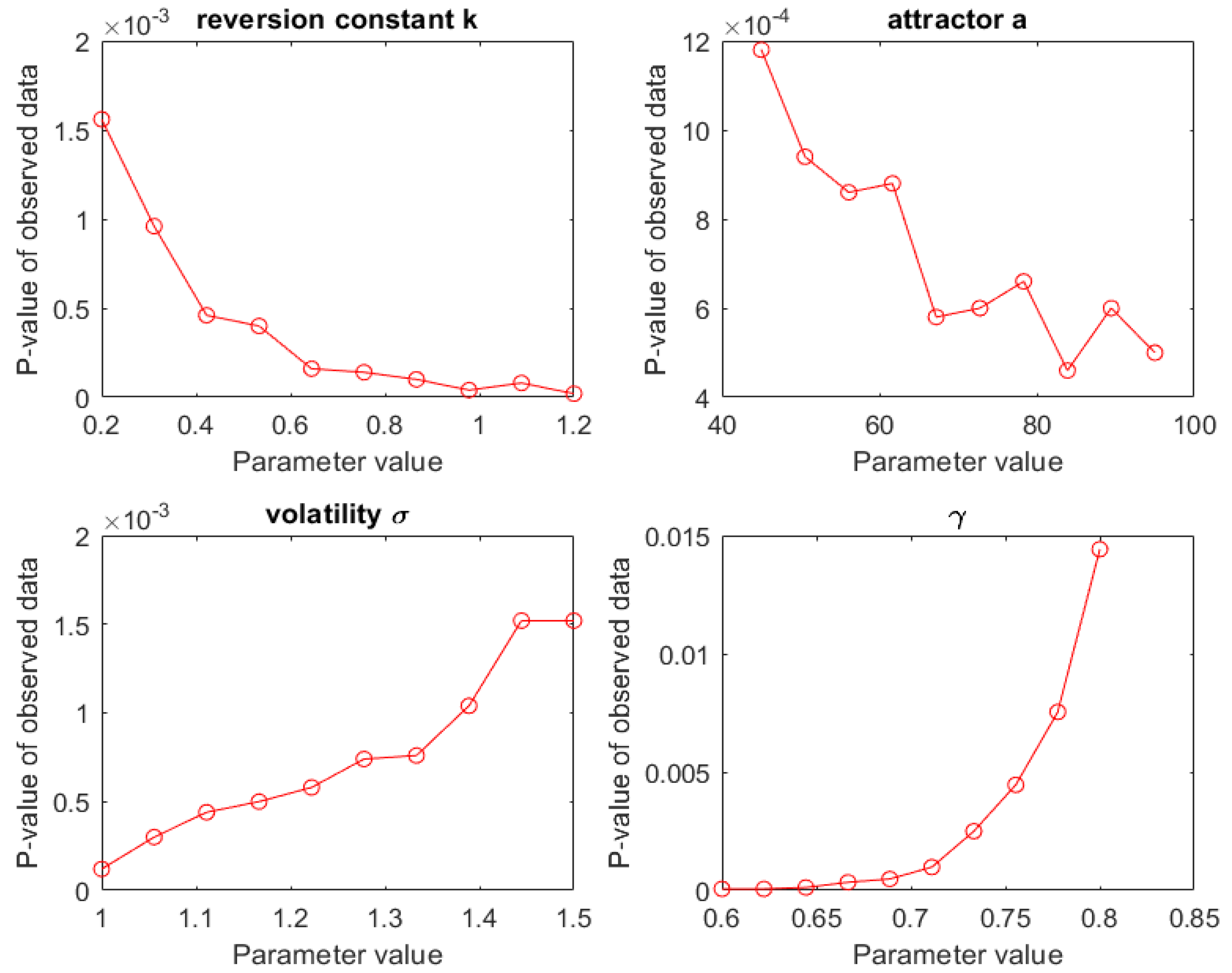
where the values for the estimated parameters are listed in Table 1. We therefore investigated, for each of the four CKLS parameters, how the p-value of the actually observed result changed as a function of changes in one selected parameter, keeping the others fixed at the estimated value. More specifically, we investigated this marginal change when the selected parameter ranged between its 5% and 95% percentiles (see Table 1, second row).
The result of this sensitivity is summarized in Figure 3, from which it transpires that the observed response remained highly significant () in all cases under marginal (i.e., single) parameter perturbations. So, from these results, we conclude that the drop in the oil price data is unusual and that this conclusion is very robust with respect to the uncertainty intrinsic to the estimation of the CKLS parameters, pointing to a significant exogenous effect.
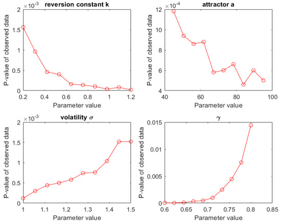
Figure 3.
Marginal sensitivity of the p-value to changes in the four parameter values. The parameters varied between their respective 10% and 90% percentiles. It turns out that the p-value remained highly significant over these ranges.
4.1.4. Corroborating the Choice of Filter Size (r)
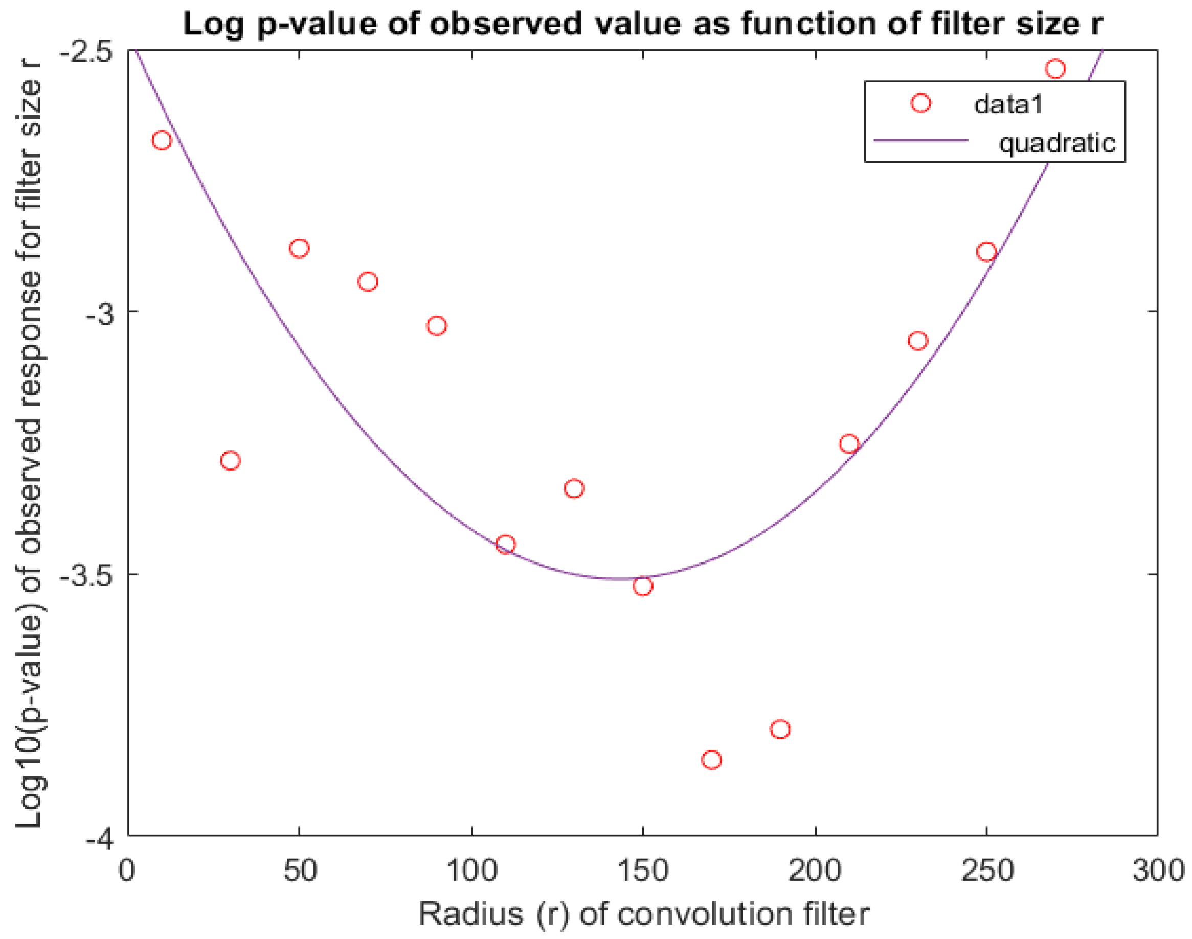
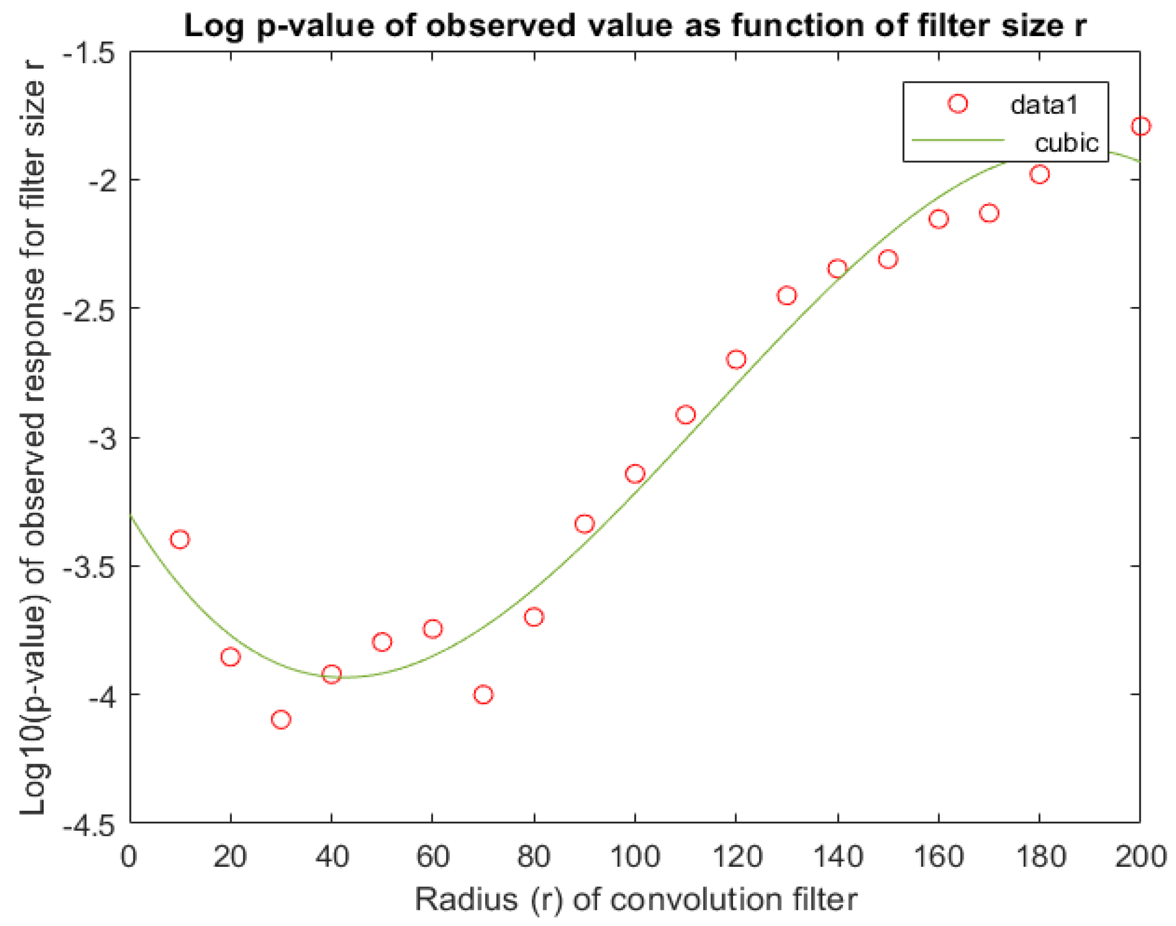
As a final check, we return to our choice of filter size () and provide additional corroborating evidence supporting this selection. Since the response depends on r we estimated the p-value for a range of r-values. To this end, we created 50,000 MC sample paths for each filter size (r) using the actual estimate of CKLS parameters (see Table 1). The results are summarized in Figure 4 from which we conclude that a filter size of about elicits a highly significant result. This observation makes sense as the conspicuous drop in oil price extends over a time period of 100–200 observations. A smaller filter will also react to shorter up or downward runs, essentially increasing the denominator in Equation (5), thus reducing the value of the test-statistic as well as its p-value. On the other hand, increasing r significantly will reduce the numerator, as the support of the filter now exceeds the length of the drop. Both these effects can clearly be seen in Figure 4 where we have plotted the 10-logarithm of the p-value of the observed test statitistic as a function of the filter size r. From this, it transpires that a choice seems appropriate.
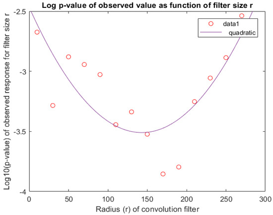
Figure 4.
p-value of observed response as function of r. From this graph, we conclude that is a reasonable choice for the filter size. The p-value for each r is based on 50,000 MC paths.
4.2. US Interest Rate (1972–2018)
As the next case study we looked at the US interest rate between 1972 and 2018 (see top panel of Figure 5). Again, there are signs of unusual and conspicuous volatility around observation 6800 that correspond to the global recession in the early 1980s. Many countries, among them, the US, experienced high inflation, interest, and unemployment rates. In order to reduce the recession consequences, the US Federal Reserve Bank decided to increase interest rates in an attempt to mitigate inflation. The resulting volatile up-swing in the time series is clearly observable, but we are interested in whether this can be reliably spotted from the data alone.
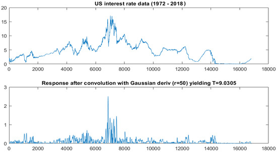
Figure 5.
Top: US interest rate data (daily results for period 1972–2018); Bottom: Response (in absolute value) after convolution with a Gaussian derivative () of size . The test statistic (the maximum value over the value of the 90% percentile, see Equation (5)) yields .
As in the previous case, we assumed that the underlying dynamics were governed by a CKLS process and we used the actual data to estimate the corresponding parameters. The resulting values are shown in Table 2 (first row). To estimate the intrinsic uncertainty of these estimates, we generated MC paths corresponding to these estimated parameters and then re-estimated the parameters based on simulated MC paths. From the resulting distribution, we were able to compute percentiles, in particular, the 5% () and 95% () percentiles, to characterize a covering interval for each of the parameters. These results are specified in the second row of Table 2.

Table 2.
US Interest Rate: estimated CKLS parameters, as well as the limits of 90% covering interval sandwiched between the 5% and 95% percentiles.
Next, we again convolve time series with a smoothed Gaussian filter of size and computed the corresponding test statistic (; the response for is shown in the bottom panel of Figure 5). To determine the p-value for this test statistic, we turned to Table 2 and plugged the estimated values for the CKLS parameters into an MC simulation. For each simulated sample path, we computed the T-value and compared it to . From this, we conclude that has a p-value of , and therefore, is highly significant. So, once again, this points to an exogenous source of variation.
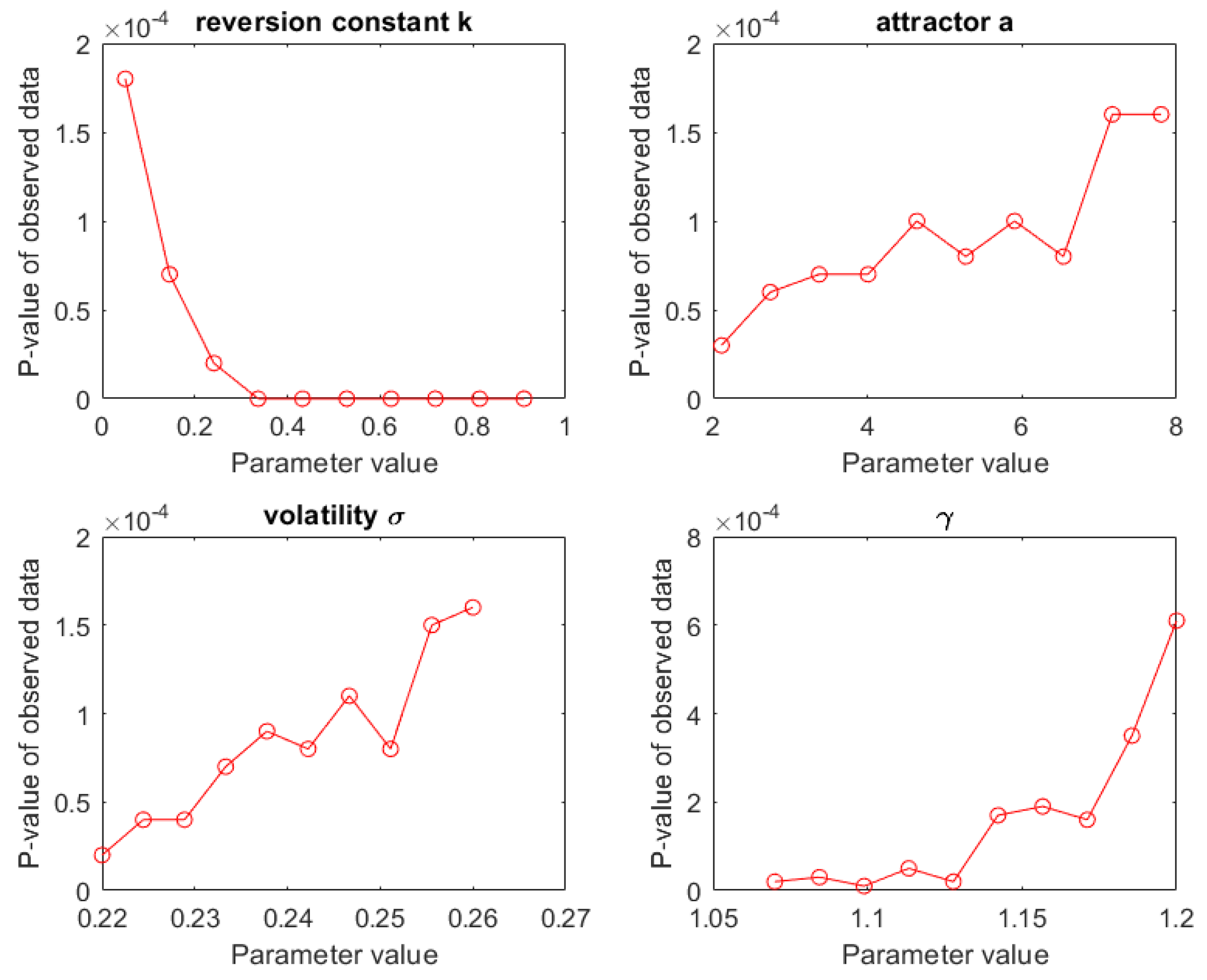
Next, we investigated how sensitive this conclusion is to changes in the CKLS parameters. In Figure 6 we varied one parameter at a time over the : ranges indicated in the second row of Table 2. From the results shown in Figure 6, it is clear that the observed value () remains significant () under these parameter ranges. As expected, has the most dramatic impact on the significance.
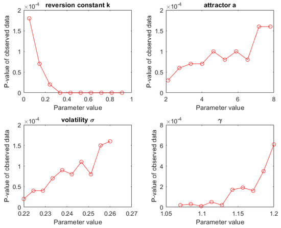
Figure 6.
Marginal sensitivity of the p-value of the response test statistic () for to changes in the four parameter values. The parameters varied between their respective 5% and 95% percentiles. It turns out that the p-value remained highly significant over these ranges.
As a final check, we used MC simulation to explore the evolution of the p-value over a range of r-values (see Figure 7). From this, it transpired that a wide range of r-values resulted in significant p-values. Hence, the precise determination of the filter size is not very important, but is definitely an acceptable choice.
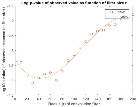
Figure 7.
Log p-values of the observed responses () as function of r. From this graph we conclude that is a reasonable choice for the filter size. The p-value for each r is based on 50,000 MC paths.
5. Discussion and Conclusions
In this paper, we investigated the CKLS processes, a family of mean-reverting stochastic processes that are widely used to model the behaviour of financial or economic assets that tend to fluctuate about a pre-defined target value. Examples include oil price and interest rates. The quantitative and qualitative behaviours of these time series are determined by four parameters that control important sample path characteristics, such as the volatility and excursion length. Because of the degrees of freedom associated with these four parameters, it is difficult to judge, by simple inspection of the data, whether or not some conspicuous feature of the time series is exceptional. To decide we needed to establish whether the observed irregularity was either well within the normal range of the process, or so unlikely as to suggest the presence of some exogenous “shock”, i.e., some perturbation outside the CKLS dynamics.
To address this question, we proposed the use of a convolution filter that resembles a smoothed Haar wavelet. Convolving the original time series with this filter allowed us to translate the observed sample path irregularities into a simple test statistic for which we were able to compute a p-value. In addition, we showed how one can then use Monte Carlo simulation to quantify the sensitivity of this p-value to the well-documented uncertainty in the CKLS parameters.
We illustrated the proposed methodology for two widely used financial time series: WTI oil price and US interest rate. In both cases, we showed that the data strongly suggest the existence of exogenous shocks: for oil price during the global financial crisis of 2008–2009 and in 1980 for the interest rate. These conclusions are consistent with the findings reported in Refs. Martín-Barragán et al. (2015); Chatzikonstanti (2017); Dewandaru et al. (2017); Naccache (2011).
So far, we have looked at the problem from a batch point of view, i.e., assuming that we have access to all relevant historical data. The logical next step is to investigate how this approach can be combined with well-known techniques for change detection (e.g., cumulative sum) to identify irregularities in running time series, e.g., to single out structural breaks. Another possible extension of the paper is to add a jump process to CKLS to see whether it improves the parameters’ performances in the presence of economic turbulence.
Author Contributions
Conceptualization, S.K., E.J.P. and A.B.D.; Methodology, S.K. and E.J.P.; Software, S.K. and K.V.M.; Data Curation, S.K.; Writing—Review & Editing, S.K. and E.J.P.; Supervision, E.J.P. and A.B.D.
Funding
This research received no external funding.
Acknowledgments
S. Kokabisaghi gratefully acknowledges partial funding by the Iranian Ministry of Science and Young Researchers Elite Club.
Conflicts of Interest
The authors declare no conflict of interest.
Abbreviations
The following abbreviations are used in this manuscript:
| BM | Brownian motion |
| CKLS | Chan, Karolyi, Longstaff, and Sanders (process) |
| GMM | Generalized Method of Moments |
| MC | Monte Carlo (estimation) |
| SDE | Stochastic Differential Equation |
References
- Aloui, Riadh, Rangan Gupta, and Stephen M. Miller. 2016. Uncertainty and crude oil returns. Energy Economics 55: 92–100. [Google Scholar] [CrossRef]
- Arora, Vipin, and Matthew Tanner. 2013. Do oil prices respond to real interest rates? Energy Economics 36: 546–55. [Google Scholar] [CrossRef]
- Bu, Ruijun, Ludovic Giet, Kaddour Hadri, and Michel Lubrano. 2010. Multivariate Interest Rates Using Time-Varying Copulas and Reducible Nonlinear Stochastic Differential Equations. Journal of Financial Econometrics 9: 198–236. [Google Scholar] [CrossRef]
- Chan, Ngai Hang, Song Xi Chen, Liang Peng, and Cindy L. Yu. 2009. Empirical likelihood methods based on characteristic functions with applications to Lévy processes. Journal of the American Statistical Association 104: 1621–30. [Google Scholar] [CrossRef]
- Chan, Kalok C., G. Andrew Karolyi, Francis A. Longstaff, and Anthony B. Sanders. 1992. An Empirical Comparison of Alternative Models of the Short-Term Interest Rate. The Journal of Finance 47: 1209–27. [Google Scholar] [CrossRef]
- Chatzikonstanti, Vasiliki. 2017. Breaks and outliers when modelling the volatility of the U.S. stock market. Applied Economics 49: 4704–16. [Google Scholar] [CrossRef]
- Chernozhukov, Victor, and Christian Hansen. 2008. Instrumental variable quantile regression: A robust inference approach. Journal of Econometrics 142: 379. [Google Scholar] [CrossRef]
- Croghan, Jakob, John Jackman, and K. Jo Min. 2017. Estimation of Geometric Brownian Motion Parameters for Oil Price Analysis. In IIE Annual Conference Proceedings. Peachtree Corners, GA, USA: Institute of Industrial and Systems Engineers, pp. 1858–63. Available online: https://search-proquest-com.eur.idm.oclc.org/docview/1951120561?accountid=13598 (accessed on 9 July 2018).
- Dell’Aquila, Rosario, Elvezio Ronchetti, and Fabio Trojani. 2003. Robust GMM analysis of models for the short rate process. Journal of Empirical Finance 10: 373–97. [Google Scholar] [CrossRef]
- Dewandaru, Ginanjar, Rumi Masih, and Mansur Masih. 2017. Regional spillovers across transitioning emerging and frontier equity markets: A multi-time scale wavelet analysis. Economic Modelling 65: 30–40. [Google Scholar] [CrossRef]
- Dutta, Anupam, Jussi Nikkinen, and Timo Rothovius. 2017. Impact of oil price uncertainty on Middle East and African stock markets. Energy 123: 189–97. [Google Scholar] [CrossRef]
- Ferrando, Laura, Román Ferrer, and Francisco Jareño. 2017. Interest Rate Sensitivity of Spanish Industries: A Quantile Regression Approach. The Manchester School 85: 212–42. [Google Scholar] [CrossRef]
- Gallant, A. Ronald, and George E. Tauchen. 1995. Specification Analysis of Continuous TimeModels in Finance. Electronic Journal, 297–321. [Google Scholar] [CrossRef]
- Grané, Aurea, and Helena Veiga. 2010. Wavelet based detection of outliers in financial time series. Computational Statistics and Data Analysis 54: 2580–93. [Google Scholar] [CrossRef]
- Hamilton, J.D. 2009. Causes and Consequences of the Oil Shock of 2007–2008. Brookings Papers on Economic Activity. vol. 40, pp. 215–83. [Google Scholar] [CrossRef]
- Hall, Alastair R., Sanggohn Han, and Otilia Boldea. 2012. Inference regarding multiple structural changes in linear models with endogenous regressors. Journal of Econometrics 170: 281–302. [Google Scholar] [CrossRef] [PubMed]
- Jain, Anshul, and P. C. Biswal. 2016. Dynamic linkages among oil price, gold price, exchange rate, and stock market in India. Resources Policy 49: 179–85. [Google Scholar] [CrossRef]
- Loisel, Sébastien, and Marina Takane. 2009. Fast indirect robust generalized method of moments. Computational Statistics Data Analysis 53: 3571–79. [Google Scholar] [CrossRef]
- MacKenzie, Donald. 2006. An Engine, Not a Camera: How Financial Models Shape Markets. Cambridge: MIT Press, p. 377. ISBN 0-262-13460-8. [Google Scholar]
- Martín-Barragán, Belén, Sofia B. Ramos, and Helena Veiga. 2015. Correlations between oil and stock markets: A wavelet-based approach. Economic Modelling 50: 212–27. [Google Scholar] [CrossRef]
- Monetary Policy Principles and Practice. Available online: https://www.federalreserve.gov/monetarypolicy/historical-approaches-to-monetary-policy.htm (accessed on 8 March 2018).
- Naccache, Théo. 2011. Oil price cycles and wavelets. Energy Economics 33: 338–52. [Google Scholar] [CrossRef]
- Ben Nowman, K., and Ghulam Sorwar. 2003. Implied option prices from the continuous time CKLS interest rate model: An application to the UK. Applied Finance and Economics 13: 191–97. [Google Scholar] [CrossRef]
- Petroleum and Other Liquids. Available online: https://www.eia.gov/dnav/pet/hist/LeafHandler.ashx?n=PET&s=RWTC&f=M (accessed on 15 August 2018).
- Salisu, Afees A., and Tirimisiyu F. Oloko. 2015. Modeling oil price—US stock nexus: A VARMA–BEKK–AGARCH approach. Energy Economics 50: 1–12. [Google Scholar] [CrossRef]
- Sorwar, Ghulam. 2011. Estimating single factor jump diffusion interest rate models. Applied Financial Economics 15: 1679–89. [Google Scholar] [CrossRef]
- Tang, Cheng Yong, and Song Xi Chen. 2009. Parameter estimation and bias correction for diffusion processes. Journal of Econometrics 149: 65–81. [Google Scholar] [CrossRef]
- Treepongkaruna, Sirimon, and Stephen Gray. 2003. On the robustness of short-term interest rate models. Accounting and Finance 43: 81–121. [Google Scholar] [CrossRef]
- Zhou, Zhongbao, Ling Lin, and Shuxian Li. 2018. International stock market contagion: A CEEMDAN wavelet analysis. Economic Modelling 72: 333–52. [Google Scholar] [CrossRef]
© 2018 by the authors. Licensee MDPI, Basel, Switzerland. This article is an open access article distributed under the terms and conditions of the Creative Commons Attribution (CC BY) license (http://creativecommons.org/licenses/by/4.0/).


