Training Set Optimization for Machine Learning in Day Trading: A New Financial Indicator

Abstract

Predicting and trading assets in the global financial market represents a complex challenge driven by the dynamic and volatile nature of the sector. This study proposes a day trading strategy that optimizes asset purchase and sale parameters using differential evolution. To this end, an innovative financial indicator was developed, and machine learning models were employed to improve returns. The work highlights the importance of optimizing training sets for machine learning algorithms based on probable asset behaviors (scenarios), which allows the development of a robust model for day trading. The empirical results demonstrate that the LSTM algorithm excelled, achieving approximately 98% higher returns and an 82% reduction in DrawDown compared to asset variation. The proposed indicator tracks asset fluctuation with comparable gains and exhibits lower variability in returns, offering a significant advantage in risk management. The strategy proves to be adaptable to periods of turbulence and economic changes, which is crucial in emerging and volatile markets.

1. Introduction

The financial market is dynamic and constantly carries out upward and downward movements in prices (called oscillations) according to internal and external influences on the financial market, shareholder sentiment, the social position of companies, government models, etc. Therefore, predicting behavior is of significant complexity. For Wang (2011), time-series prediction for financial markets can be considered one of the main challenges in the literature in the machine learning segment.

It is not wrong, nor a corruption of ethical principles, to make money. Consequently, investing in shares in the financial market attracts more and more people interested in extra but variable risk-prone income. These people are responsible for the movement of the financial market, as they influence and are influenced at every moment.

For Cavalcante et al. (2016), an investor’s success depends on the quality of the information used to support decision-making and how quickly this investor can make decisions.

Si and Yin (2013) raises the issue that many works treat time series in financial markets as linear; however, their research defines it as essentially complex, highly noisy, dynamic, non-linear, non-parametric, and naturally chaotic.

In this context, predicting asset variations in the financial market is highly complex. A wide range of techniques and models are being researched and discussed to maximize returns and minimize risks.

From the Hsu et al. (2016) study, a hypothesis is generated for the thesis proposal that there are groups of investors with similar investment patterns, and whether based on speculation, investment techniques, feelings, etc., these investment behaviors influence asset fluctuations. Therefore, in this context, it is possible to assume that there are correlated movements in specific time windows. It is believed that it is possible to improve prediction models through correlated time series, developing a robust model for daily asset trading.

Still, according to Hsu et al. (2016), several hypotheses about financial market prediction are listed, being validated or refuted based on previously published research. One of the hypotheses raised in the study is about the correlation between the models’ input and output, stating that the higher the correlation, the better the results.

This paper aims to create a prediction model that optimizes training sets for machine learning algorithms for trading financial market assets in daily operations, with clustering and machine learning techniques as the central studies.

This paper seeks to fill this gap by proposing a prediction model that dynamically optimizes training sets for machine learning algorithms, specifically for day trading operations in financial market assets. The main approach involves combining clustering techniques to identify market behavior patterns and machine learning to predict stock fluctuations in day trading operations.

Financial market assets can exhibit behavioral variations over time, making optimization and trading strategy adjustments important.

Long-term tests are necessary to understand the dynamics of the trading strategy. In this experiment, the strategy is tested with a real database, with an asset from an emerging market over almost seven years, going through several turbulences, such as the impeachment of a president, change in economic management, COVID-19, etc. Strategies based on behavioral changes (adaptive) are not widely explored in the literature but are essential for the evolution of consistent research.

Another important factor to be discussed is that the selection of training sets is widely studied in academia and applied to several problems, as in Hammoudeh and Lowd (2024), Chang et al. (2021) and Ramezan et al. (2021); however, for computational finance, it is not widely explored, with this being one of the main aspects of this study.

This paper seeks to fill this gap by proposing a prediction model that dynamically optimizes training sets for machine learning algorithms, specifically for day trading operations in financial market assets. The main approach combines clustering techniques to identify market behavior patterns and machine learning to predict stock fluctuations in day trading operations.

This study proposes and demonstrates that it is possible to develop strategies that adapt to changes in the behavior of financial market assets. Strategies and models of a technique based on machine learning may not work for a long time in a highly volatile issue. For this reason, algorithms must undergo adjustments over time, shaping and optimizing parameters continuously so that they can continue to present good results.

2. Research Problem

Identifying patterns in the upward and downward movements in the price of assets in the financial market has always been a challenge for all areas of knowledge, as their variations depend on several factors, such as the economy, historical price behavior, the fact that investors who move the market are subject to varied emotions, etc. Such emotions, such as fear and greed, can interfere with buying and/or selling.

To assist investors in choosing and monitoring their assets, many statistical and machine learning techniques have been studied and applied to minimize prediction errors and investment risks.

The problem addressed in the thesis is to generate a daily trading model based on the historical behavior of the asset, applying techniques to optimize the training set for applying machine learning techniques. A trading model is developed to create scenarios of the daily movements of an investment, evaluate the gain from the method, and generate a new financial indicator.

Thus, the problem was segmented so that it can be treated in a modular way by the study.

• Scenario Detection Modeling (Clustering): Identification of different scenarios (behavior patterns) helps machine learning techniques obtain better results. In this way, it is proposed to answer the question: What is the best way or method to segment scenarios of asset market variations?
• Predictive Modeling: There is a wide range of research into predictive modeling for the financial market. Can we segment scenarios and use them to optimize training sets to improve asset prediction?
• Operation Model: One of the main challenges for studies relating to the financial market is how to use information to model entry and exit points. In this thesis proposal, the following questions arise: Is it possible to optimize return results? How can we create and optimize an operating model?

This research proposal aims to create a prediction model that optimizes training sets for machine learning algorithms for trading financial market assets in daily operations, with clustering and machine learning techniques as the central studies. The main contributions of this study are the following:

• To develop a model to segment asset variation scenarios in financial markets.
• To develop a financial indicator based on an asset’s daily behavior.
• Creation of a trading model based on clustering and prediction techniques to generate a set of rules for daily asset operations.

3. Related Works

According to Mintarya et al. (2023), there are two significant theories in the stock market: the Efficient Market Hypothesis (EMH) and the Random Walk Theory. However, it is possible to use machine learning techniques to overcome these paradigms. In their survey, they observed that half of the studies for stock market forecasting had used long short-term memory (LSTM) or support vector machine (SVM) since 2012.

DiPersio and Oleksandr (2017) used Google sStocks to forecast variations for a five-day horizon, applying three basic recurrent neural network (RNN) techniques, LSTM, and the gated recurrent unit (GRU). LSTM outperformed the other methods with an accuracy of $72\%$. The study by Roondiwala et al. (2017) shows that the LSTM result achieves an RMSE of 0.00859 for test sets for daily variation assessments. According to Shah et al. (2019), LSTM has proven to be very efficient for forecasting time series in the stock market.

Liu and Wang (2018) use a deep neural network (DNN) for intraday stock prediction; the study compares a DNN with an artificial neural network (ANN), and daily predictions are optimized by 8–11%.

Carvalho et al. (2024) use a decision tree to extract sets of movement rules to interpret the results in day trading operations. The simplicity of the technique and ease of interpretation of the set of rules made it an interesting study, reaching an accuracy of 53.96%.

A diverse range of models in the study of Nabipour et al. (2020), including tree-based models (decision tree, bagging, random forest, Adaboost, gradient boosting, and XGBoost) and neural networks (ANNs, RNNs, and LSTM), were employed to accurately predict various segments of the stock market. This comprehensive approach ensured a thorough exploration of the predictive modeling landscape. Classification and regression models were used to forecast the variations in different time horizons, with LSTM demonstrating the best performance.

Hegazy et al. (2014) proposed a machine learning model integrating the Particle Swarm Optimization (PSO) algorithm and least square support vector machine (LS-SVM) for stock price prediction using financial and technical indicators. These indicators include relative strength index, money flow index, exponential moving average, stochastic oscillator, and moving average convergence/divergence. The PSO is employed iteratively as a global optimization algorithm to optimize LS-SVM for stock price prediction. The proposed LS-SVM-PSO model is capable of overcoming the over-fitting problem found in ANNs. PSO-LS-SVM algorithm parameters can be tuned easily. The performance of the proposed model is better than that of LS-SVM and compared algorithms. LS-SVM-PSO achieves the lowest error value followed by a single LS-SVM, while the ANN-BP algorithm is the worst.

Studies indicate that the best machine learning method is LSTM. However, most studies do not train machine learning techniques based on a trading strategy. They only use the prediction result to assess whether the asset is bought or sold.

In our study, a trading strategy is developed, and a training model is adjusted for each new market movement. We place a strong emphasis on the selection of data for the training sets of machine learning models, as it is based on probable behaviors of the assets (scenarios). This approach ensures that our model is well informed and ready to adapt to market changes.

4. Materials and Methods

A framework model was developed, Figure 1, segmented into four stages, and subdivided into several stages, including (I) data acquisition and processing, (II) scenario segmentation, (III) prediction model, and (IV) modeling strategies and performance metrics.

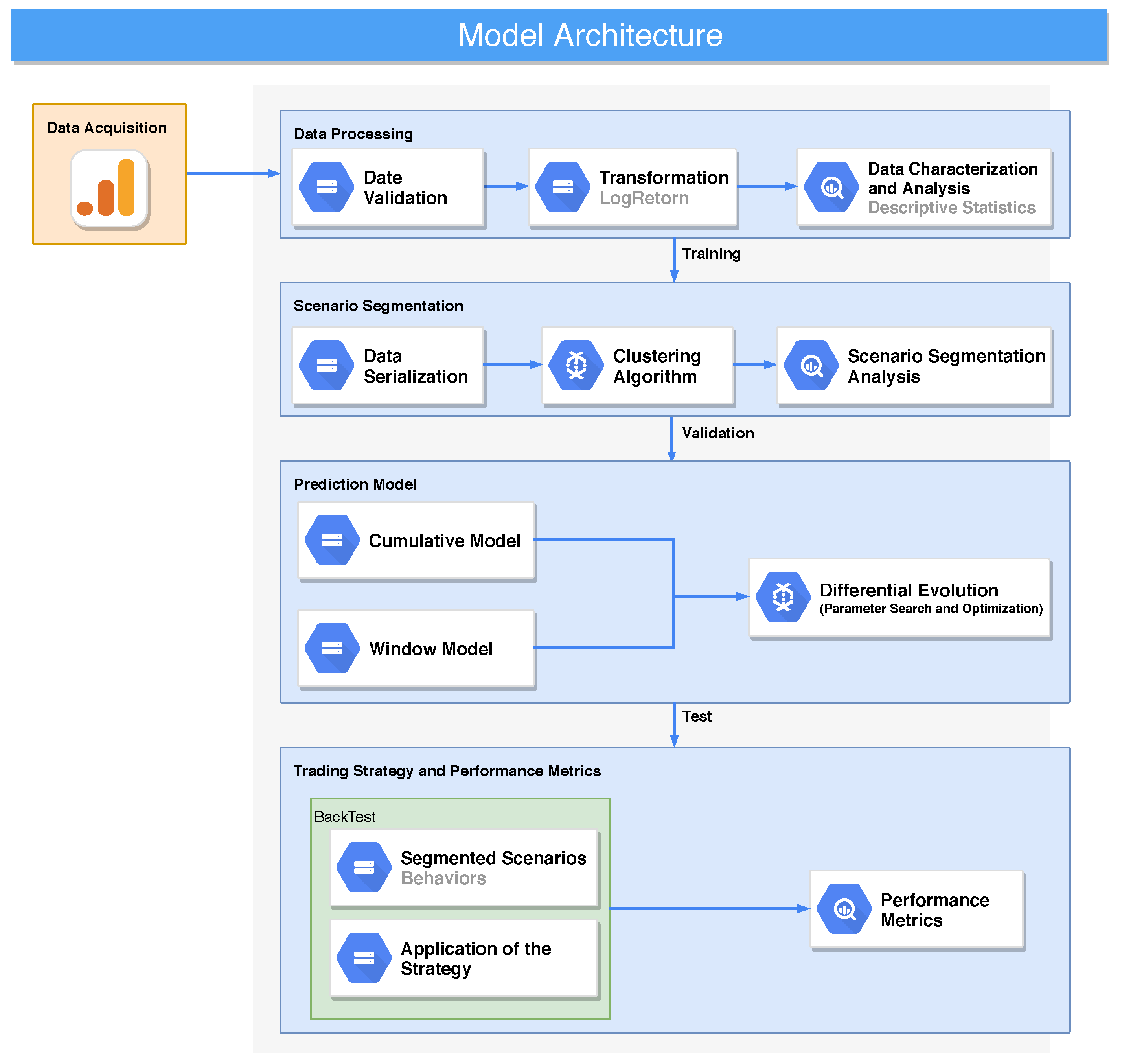
4.1. Data Acquisition and Processing

Brazilian market (${\left[B\right]}^3$) real data were used, Bovespa Index Future [WIN$N], at fifteen-minute intervals from “Jan/2014” to “May/2021”. The dataset can be accessed at the following link: https://github.com/AngeloDarcyMS/dataBovespaWIN_20142021 (accessed on 14 May 2025).

There are $67.323$ data lines containing the date, time, opening, maximum, minimum, current closing, trading volume, number of securities, and spread.

The objective of the data processing acquisition step is to perform three main steps.

• Normalize the input data;
• Completely delete days for which there are missing data;
• Build a structure for the remaining steps.

The financial returns are computed in points, not currency, and are based on the original data, not the normalized data.

The structure generated in this step has two sets of data that are accessed vectorized. One set contains the normalized data, and the other contains the original data.

In this study, an intraday investment strategy is proposed, with the daily curves of the asset normalized based on the variations for each day. For cumulative returns it is necessary to normalize the data to a log-return scale (Tsay (2014)), Equation (1).

$$l_t=ln\left({\displaystyle \frac{p_t}{p_i}}\right)$$

(1)

t is the instant of return, i the initial instant of time, and $l-t$ the normalized return obtained between the instant i and t.

Instant i represents the beginning of the day, and instant t is the reading sequence of the asset variation on the day. Thus, each new reading is always normalized according to the initial reading of the day.

4.2. Modeling of Scenario Segmentations

Scenarios in this study are called similar daily behaviors; thus, this step aims to determine the possible scenarios for the assets. The main methods are the following:

• Data Serialization: consists of the organization of the data according to the time granularity of the searched base in this study of 15 min.
• Clustering Algorithms: execution of the algorithm that defines the scenario segments of the assets.

Clustering is a data mining technique in which similar data is placed into related or homogeneous groups without advanced knowledge of group definitions Rai and Shubha (2010). Its main objective is to maximize the similarity of grouped objects and minimize the similarity between groups.

In this study, we adopt the Agglomerative Hierarchical Clustering method to define scenarios, the correlation between the days in the training set to assemble the distance matrix (dissimilarities), and the distance parameter between the cluster’s average centroids.

The advantages of hierarchical clustering include Berkhin (2006).

• Flexibility regarding the level of granularity;
• Ease of handling any form of similarity or distance;
• Applicability to any attribute type.

The disadvantages of hierarchical clustering are

• The difficulty of choosing the right stopping criteria;
• Most hierarchical algorithms do not revisit (intermediate) clusters once they are constructed.

The hierarchical clustering algorithm initially treats all individuals as clusters, and clusters are generated from the union of individuals/clusters. In this study, the correlation was used as the configuration to calculate the distance metric, and the average was used as the linkage method. This algorithm is flexible; it does not have the definition of the number of clusters as parameters, and its principal characteristic is that it is interpretable through the dendrogram.

Financial market assets, such as the case study in this research, are highly volatile, generating behaviors that can be described as atypical (outliers). Based on this concept, a cutoff point based on a percentage of days allocated to clusters is used as the stopping criterion. Thus, when the algorithm groups approximately $80\%$ of the individuals (daily behaviors), the algorithm is terminated since the remaining data are considered highly volatile, have a low contribution, and do not present important behavioral characteristics.

In our study, for the application of the algorithm, no limit is generated for the number of clusters, meaning that each new set of clusters that will be used does not have a fixed size.

Dynamic Time Warping (DTW) techniques are not used to apply this algorithm, as there are few points to be clustered, and time alignments (or time shifts) would harm the Financial Representativeness Indicator.

4.3. Modeling the Prediction

The model consists of predicting the asset at the end of a day (or period). Two parameters are used for this: estimated financial return (FR) and similarity.

The financial return estimate ($FR$) is performed at each fifteen-minute reading, considering the correlation of daily behaviors (clusters) and the reading of the day it is being analyzed. Thus, there is adaptability and correction of estimates during asset negotiations.

Equation (2) computes the estimated financial return of the instant i by the end of the day ($F{R}_i$), where i is the valuation instant of the trade, n the number of scenarios, c represents the scenario (cluster), P is the representativeness of a Scenario c, and G is the estimated financial return in Scenario c.

$$F{R}_i={\displaystyle \frac{{\sum }_{c=1}^n{G}_c{P}_c}{{\sum }_{c=1}^n{P}_c}}$$

(2)

Equation (3) is the similarity estimate from the beginning of the day to the moment i ($Similarit{y}_i$) considering the amount of n scenarios, where c represents the scenario (cluster), P is the representativeness of a Scenario c, and S is the correlation between the curve of the day until moment i and the curve of cluster c.

$$Similarit{y}_i={\displaystyle \frac{{\sum }_{c=1}^n{S}_c{P}_c}{{\sum }_{c=1}^n{P}_c}}$$

(3)

To generate a return estimate for the Representativity model, the Equations (2) and (3) are used; with the weighted average of the scenarios in which they have a behavior similar to the reading of the asset, the similarity is represented by the sigma in Figure 2, taking into account the scenarios that correlate with the current reading greater than sigma. $\overline{D}(FR,Similarity)$ represents the resultant vector position from which it will be used to compose the model’s strategy.

For the prediction models based on machine learning, data from scenarios with $similarity>\sigma$ are used, acting as a filter for training the learning models, making them have a better estimate, which is one of the main contributions of the work. It is a simple strategy, but it can optimize the training set, making the training faster and improving the financial return.

Tests were generated using time windows for six, twelve, and twenty-four months and a model using all past data (cumulative).

Three techniques are applied to predict machine learning-based models: support vector regression (SVR), multilayer perceptron (MLP), and long-sort term memory (LSTM).

Support vector regression (SVR) is a regression technique based on support vector machines (SVMs), which seeks to find a function that has, at most, one deviation ɛ from the real target values for all training data and at the same time is as flat as possible. The model is formulated as a convex optimization problem and can be extended to capture non-linear relationships using kernel functions, Vapnik (2013).

Si and Yin (2013) define financial market time series as highly complex, non-linear, and very noisy. For this reason, the Radial Basis Function (RBF) was chosen because it behaves well with non-linear relationships.

To apply the SVR (RBF), it is necessary to configure three parameters which influence the learning behavior of the model. These are C, epsilon, and gamma.

The C parameter controls the model’s penalties; a high value can generate overfitness for the model, which can harm the analyses. For this study, the data were normalized. During the tests, the C parameter was varied, and in the end, it was defined as 2. The $gamma$ parameter, which defines the influence of an individual training point and has a low value of $0.1$, was defined and seeks to generate a lower risk of over-fitness. The $epsilon$ parameter, which defines the size of the tolerance range where errors are not penalized, was defined as $0.1$.

A multilayer perceptron (MLP) is a feedforward artificial neural network model that maps sets of input data onto a set of appropriate outputs. It consists of multiple layers of nodes in a directed graph, each fully connected to the next one. MLPs use a supervised learning technique called backpropagation for training the network, Haykin (1994).

For the application of the MLP, the configurations applied for the experiment were two hidden layers $(64,32)$, using ‘$relu$’ as the activation function, ‘$adam$’ as the optimization algorithm, a learning rate of $0.001$, and the $L2$ regularization term, alpha, at $0.001$.

Long short-term memory (LSTM) networks, a specific class of recurrent neural networks (RNNs), were developed in Hochriter and Schmidhuber (1997). They were designed to address a significant challenge in traditional RNNs—the issue of ‘gradient fading’ that hampers the learning of long-term dependencies in time series and sequences of data.

For the application using LSTM, two dense hidden layers with 68 units were used, with ‘adam’ as the optimization algorithm, a maximum of 20 epochs, dropout equal to $0.2$, a learning rate at $0.001$, early stopping applied using the ‘val_loss’ parameter, and batch size fixed at 32.

4.4. Trading Strategy and Performance Metrics

Figure 2 represents a new model for day trading strategies. The model initially represents a simple way to merge two important parameters for asset trading. Financial return, which is the basis of any trading strategy, and similarity, which identifies past behaviors similar to the asset’s behavior during the day’s trading on the stock exchange.

The trading strategy is based on two main parameters ($\alpha$ and $\sigma$), through these parameters the regions of operation are listed. The $\alpha$ parameter (${\alpha }_1$ and ${\alpha }_2$) indicates the estimated financial return, and the $\sigma$ parameter (${\sigma }_1$ and ${\sigma }_2$) indicates the similarity of each scenario (behavior) with the asset during the course of the day on the stock exchange.

Scenarios that do not correlate with sigma’s values are not taken into account for the trading strategy. It is in what is called the region of uncertainty. The region of uncertainty is vital for an asset trading model.

Many researchers consider the financial market as a problem of high noise, dynamic and chaotic. It is crucial to create the identification of moments of non-operation, indicating behaviors of market instability.

Trading strategies can operate in two moments, long and short trades, with the trader “betting” that the asset will rise/fall in value. Thus, estimates of financial return above or below the $\alpha$ parameter (${\alpha }_1$ and ${\alpha }_2$) will indicate moments of buy or sale of the asset, called the operation region.

Figure 2 contains an example of the strategy’s behavior during the day used in the representation strategies. Based on the similarity estimates of scenarios A, B, and C, the estimator $\overline{D}(FinancialReturn,Similarity)$ is generated, using Equations (2) and (3).

Scenario A has greater representativeness than scenarios B and C, making the estimator $\overline{D}$ have a smaller vector distance in relation to Scenario A.

For strategies based on machine learning, scenarios with a parameter $Similarity\ge \sigma$ are used as a training set.

For each day of the test set, a financial return prediction for the end of the day is generated at each fifteen-minute reading. Thus, the strategy adapts to market conditions, allowing you to adjust buy/sell positions during the trading session.

Differential evolution is used as an optimization technique and search for the $\alpha$ and $\sigma$ parameters because the financial returns are dependent on these parameters. Variations in these parameters are necessary to adapt to fluctuations in the financial market.

Using evolutionary algorithms for search and optimization problems, it is possible to operate in two main areas: (I) diversification—search in spaces not known by the population—and (II) intensification—search in promising regions found by the population.

In this study, differential evolution is used to intensify a promising operating region by optimizing the $\alpha$ and $\sigma$ parameters of the operation strategy.

The readings are performed at fifteen-minute intervals, and for each reading the behaviors with similarity greater than $\sigma$ are set and the financial return estimated.

The population is represented by the four parameters to be optimized (${\sigma }_1$,${\sigma }_2$,${\alpha }_1$,${\alpha }_2$), and for each individual in the population the fitness is calculated based on the financial return in the last month ($Max\left(Return({\sigma }_1,{\sigma }_2,{\alpha }_1,{\alpha }_2)\right)$). The population for each new month is represented by a random variation in the best parameters used in the last month, so for each new month a search is made based on the intensification of promising regions, minimizing the diversification of the search and the number of generations needed, allowing fine adjustments in the parameters minimizing the problems of border regions.

Scenario modeling performance metrics are evaluated in two ways.

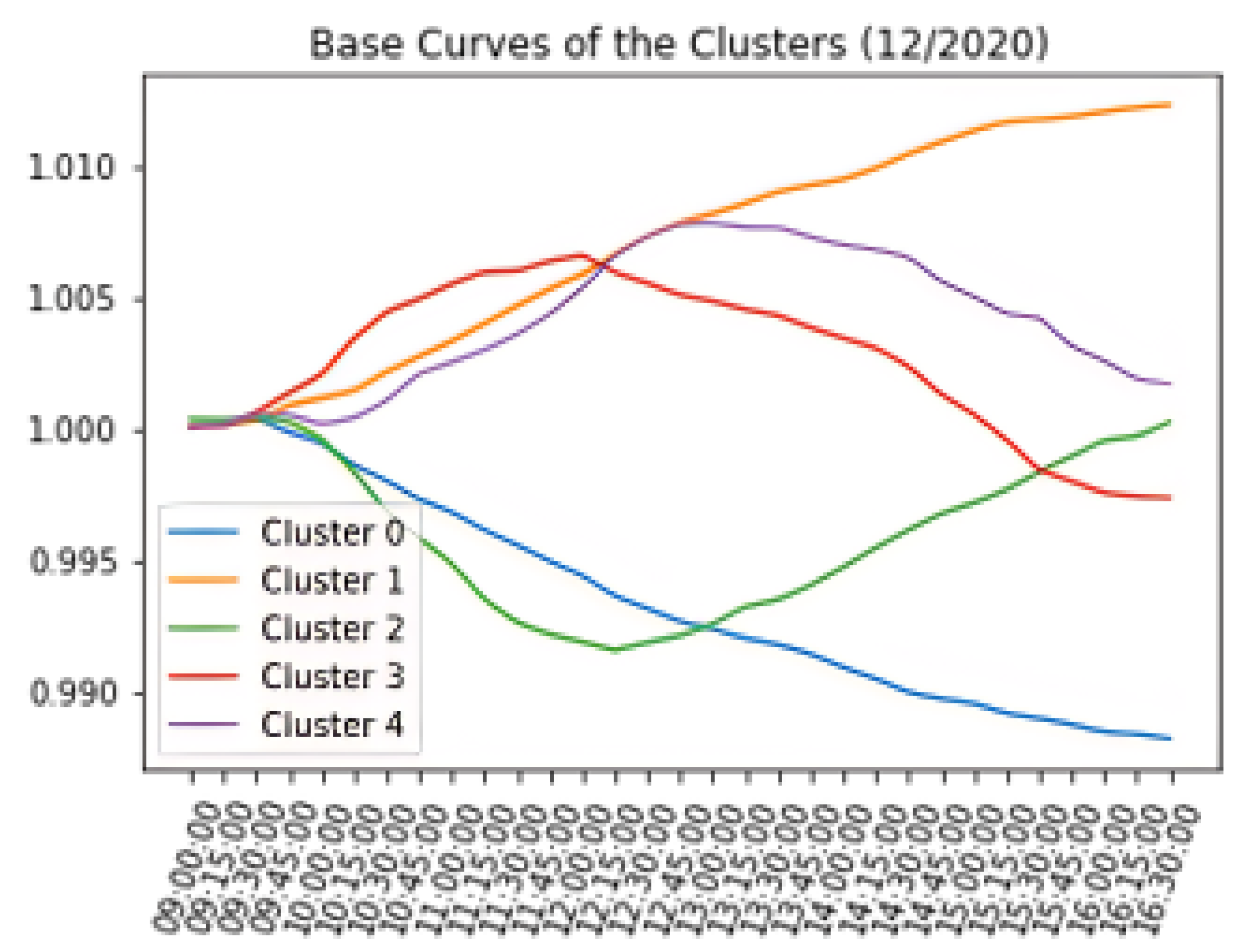
• Observing the cluster (scenarios) created, their representations, and the distribution of the curves;
• The correlation between clusters.

Performance metrics for the trading strategy are evaluated in four ways:

• Financial Return: Based on the gain or loss on the transaction and return points, with the difference in points of the buy and sale negotiations;
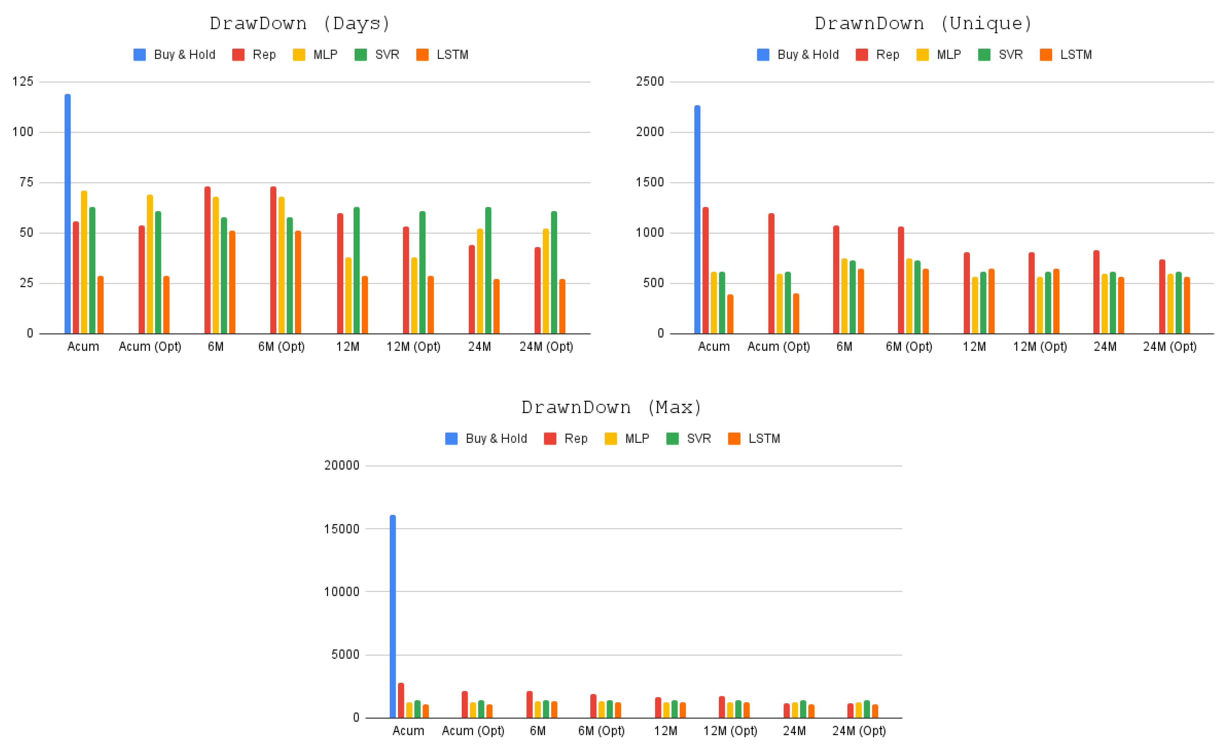
• DrawDown (Days): It represents the maximum number of consecutive days when the strategy operated with negative profit after any drop;
• DrawDown (Max): A maximum accumulated loss that the strategy generated;
• DrawDown (Max Unique): A maximum loss in an unique day.

The tests are divided into cumulative and windows, and for each test the optimization of parameters with DE is applied, described by Optimized in the results.

• Cumulative: All daily curves are added to the model before the current test month;
• Window: Represented by data six, twelve, and twenty-four months before the current test month.

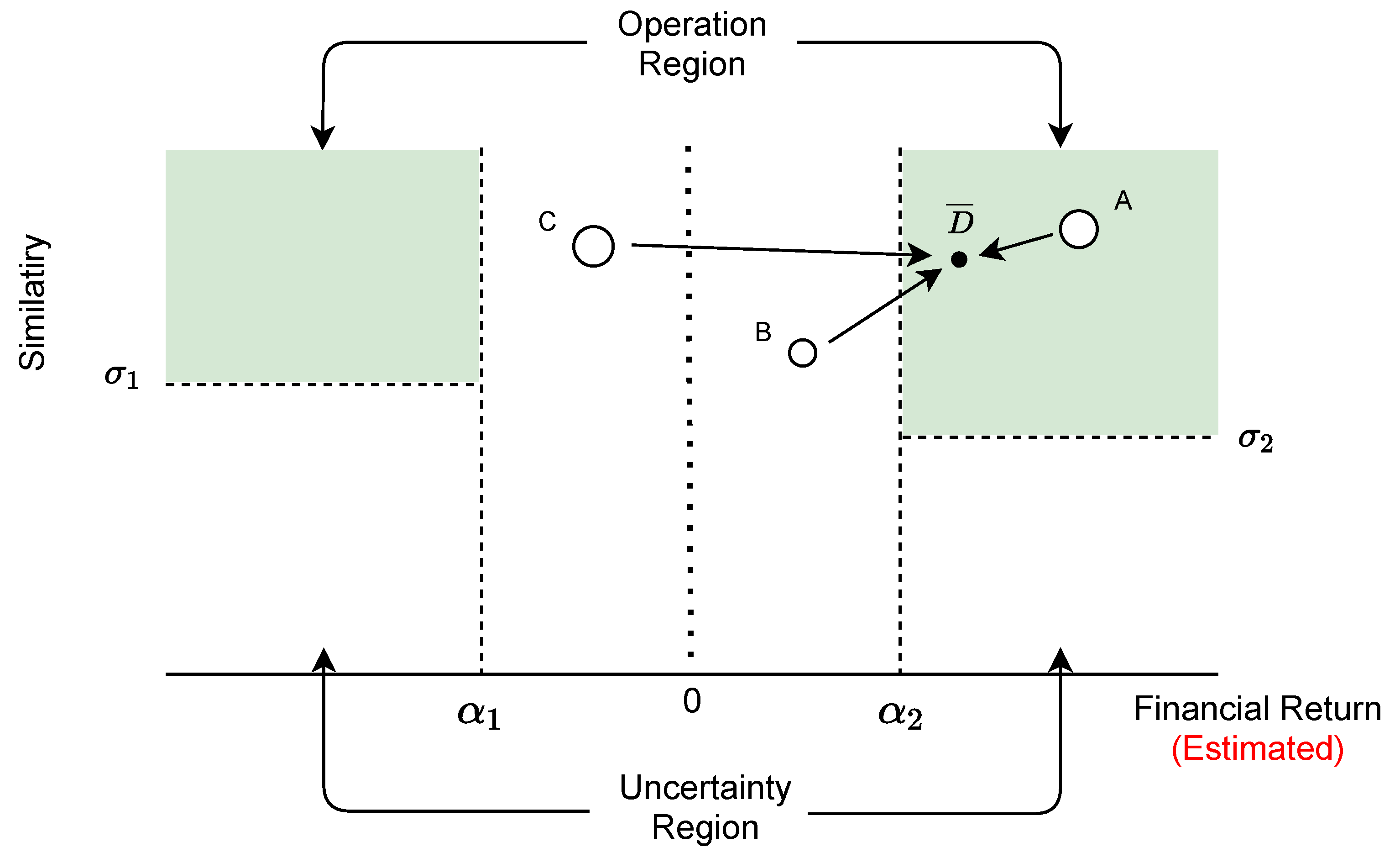
4.5. Financial Indicator: Representativeness

The representativeness financial indicator uses the asset’s past behavior to create possible behavior profiles, called scenarios.

Using these scenarios, we weigh the estimates of financial returns by the proportion of each scenario about all probable scenarios for the asset on the day, and we have an estimate of the daily return.

The systematic sequence of actions, outlined in Algorithm 1, is employed to compute the representativeness financial indicator metric. This method, along with the sequence to generate purchase and sale operations, is detailed in Section 4.4, ensuring a reliable and consistent approach.

This financial indicator requires three parameters: horizon of past observed data, similarity parameters ($\sigma$), and estimated financial return ($\alpha$).

The observed data horizon parameter aims to identify asset behaviors. In the experiments carried out in Section 5, different horizons were treated, and performance metrics were analyzed.

The similarity and financial return estimate parameters indicate times for the buying or sale of assets.

Algorithm 1: Simulation and Real Operation

Reading of daily asset data depending on the window horizon Create clusters to identify standard asset behaviors Evaluate performance metrics for each Cluster Created for Each day of the dataset do     for each new reading of 15 min do         Compute the Similarity of the asset’s current Curve with the base of existing clusters (Scenarios)         Uses data from Scenarios with $Similarity>\sigma$ to compute the Estimated Return         if there is no Buy and Sale movement for the asset then            if the Estimated Financial Return is higher than ${\alpha }_1$ then                Buy movement is activated            end if            if the Estimated Financial Return is lower than ${\alpha }_2$ then                the Sell movement is activated            end if         end if         if the Asset is Buy then            if the Estimated Financial Return is lower than ${\alpha }_2$ then                Sell movement is activated            end if         end if         if the Asset is Sold then            if the Estimated Financial Return is greater than ${\alpha }_1$ then                Buy movement is activated            end if         end if         15 min before the market closes, complete all operations     end for end for

5. Experimental Setup and Result Analysis

Our experimental results, which hold significant implications for daily assets’ behaviors and financial return, are divided into two key parts: (I) characterization of daily assets’ behaviors (scenarios) and (II) financial return based on the proposed model.

The experiment was performed using only a single contract to make a realistic comparison with the baseline; the potential for maximizing results is possible, which is a motivating factor for future research. This can be achieved by operating more contracts or leveraged operations, offering a promising avenue for enhanced performance, which is not addressed in this study.

Behavior changes are natural in the stock market. The low representativeness of some clusters makes the model delay the exit of a position. The stop loss is used to anticipate the closing of the position. It was fixed at $1\%$ due to empirical observations during the experimental evaluation phase. The stop loss was implemented based on the variation of the start of the operation for each new reading of the asset. If the financial return (points) is lower than the stop loss, the asset position is closed using the opening value of the asset in the candle.

Thus, a stop loss is used to anticipate the closing of the position, being set at $1\%$ due to empirical observations during the experimental evaluation phase.

5.1. Characterization of Daily Assets’ Behaviors (Scenarios)

Figure 3 consists of examples of segmentation scenarios (training set) when the experiment setup was run for twenty-four-month windows in January 2021. For each new month, past clusters are forgotten, and new sets of behaviors (clusters) are observed and used to run the algorithm applied in the research.

It is interesting to inspect the dynamics of the scenarios over time; it is possible to observe the market’s behavior. Visualizing clusters at different times can comprise the dynamics of the market and how the adaptation of the proposed model works.

In all analyzed periods, the scenarios with the most significant representation were the downward and upward trends. Market reversal moments occur with less ownership but are extremely important for the strategy developed by this research because the combination of scenarios indicates the best time to move into or out of position.

In Figure 4, we observe the average behavior of the scenarios. This behavior will be used to analyze the similarity at each new reading of the cycle (day) with the possible scenarios for the assets.

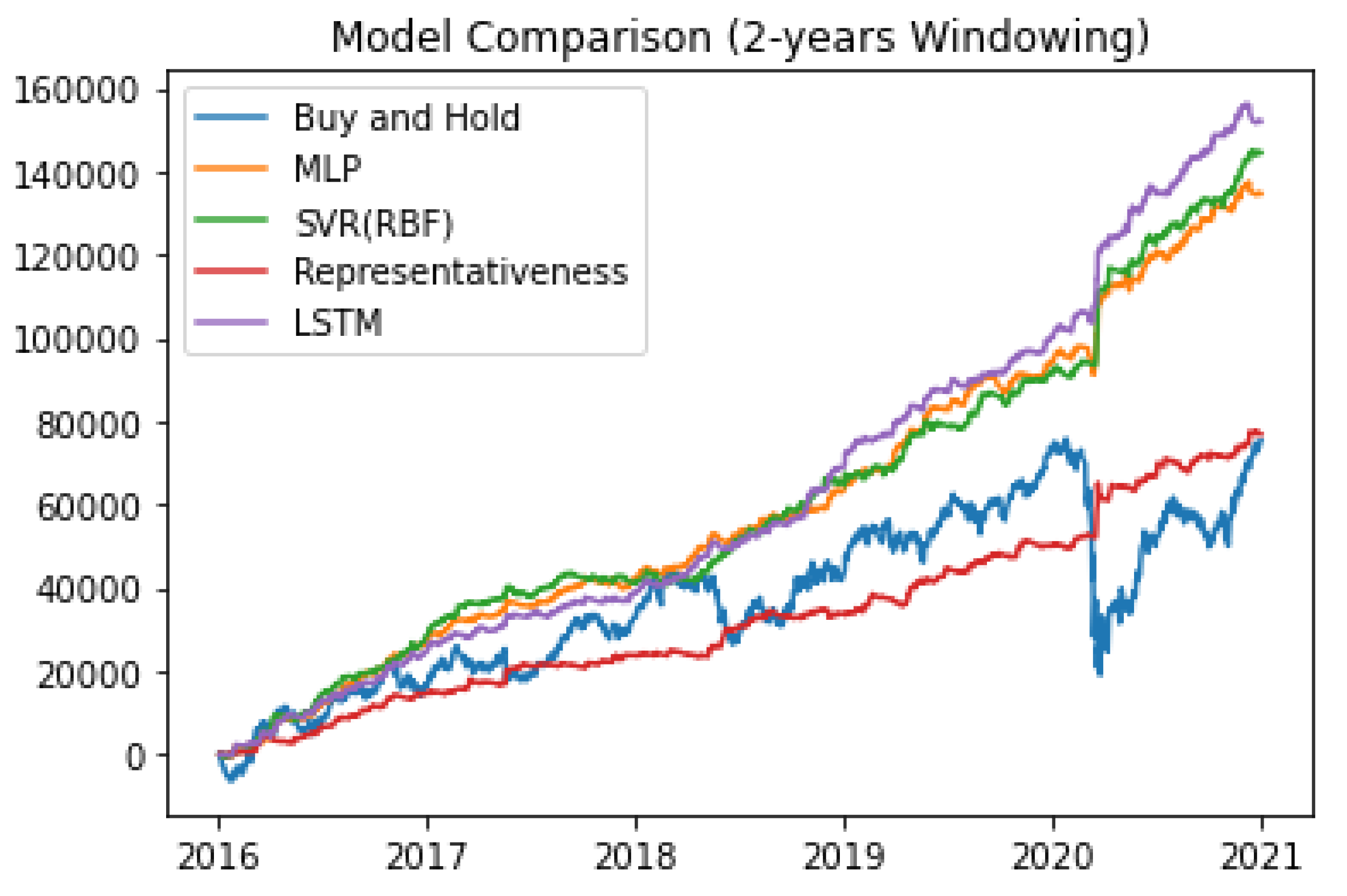
5.2. Financial Returns Based on the Proposed Model

Table 1. Experimental results.

	Time Horizon	FR	DrawDown (Days)	DrawDown (Max)	DrawDown (Unique)
B. & H.		75.652	119	−16.080	−2.265
Rep	Acum	76.265	56	−2.837	−1.263
	Acum (Opt)	76.323	54	−2.120	−1.198
	6 M	76.486	73	−2.126	−1.072
	6M (Opt)	76.543	73	−1.879	−1.068
	12 M	76.645	61	−1.628	−807
	12M (Opt)	76.726	60	−1.747	−807
	24 M	76.838	44	−1.215	−834
	24M (Opt)	77.234	43	−1.209	−734
MLP	Acum	126.424	71	−1.254	−612
	Acum (Opt)	126.578	69	−1.254	−592
	6 M	132.789	68	−1.351	−552
	6M (Opt)	133.089	68	−1.351	−552
	12 M	133.687	38	−1.287	−562
	12M (Opt)	133.687	38	−1.287	−562
	24 M	134.692	52	−1.220	−592
	24M (Opt)	134.756	52	−1.220	−592
SVR	Acum	127.543	63	−1.441	−612
	Acum (Opt)	127.564	61	−1.441	−612
	6 M	134.265	58	−1.441	−623
	6M (Opt)	134.265	58	−1.441	−623
	12 M	144.398	63	−1.387	−612
	12M (Opt)	144.452	61	−1.441	−612
	24 M	144.531	63	−1.387	−612
	24M (Opt)	144.565	61	−1.441	−612
LSTM	Acum	129.504	29	−1.102	−483
	Acum (Opt)	129.566	29	−1.102	−398
	6 M	135.689	51	−1.316	−451
	6M (Opt)	136.786	51	−1.263	−451
	12 M	149.823	29	−1.223	−649
	12M (Opt)	149.897	29	−1.223	−649
	24 M	152.345	27	−1.126	−566
	24M (Opt)	152.405	27	−1.126	−566

presents each segment’s results. The methods are based on representativeness and use the MLP, SVR, and LSTM machine learning techniques. Windows are used for each model: cumulative (Acum), six months (6 M), twelve months (12 M), and twenty-four months (24 M) past as a training set. Results were generated for all tests without optimization and with parameter optimization (Opt).

In all cases, the experiments’ results are better than the baseline when observing the DrawDown parameter. Buy-and-hold has a DrawDown (max) of $16.080$ points. The worst performance of the experiments is related to the cumulative representativeness financial indicator, presenting a value of $2.837$ points, a drop of approximately $82\%$. This financial parameter is essential, as it demonstrates the worst accumulated loss generated by the strategy from any point in the asset’s history. This is a powerful point for the financial representativeness indicator.

Trading strategies can be aggressive or conservative; the proposal for the financial representative indicator is that it is a conservative indicator, as it waits for the market to act to indicate the moment of purchase/sale, and therefore its purpose is to present constant gains even if the market is reacting negatively.

Another substantial gain of the model is related to the number of days it remains with negative gains from a fall in DrawDown (days). The results were better in all applications using machine learning, reaching only 27 days. This can be considered a great result in a market with high volatility.

The superiority of strategies employing machine learning techniques over the model relying solely on representativeness and buy and hold is evident. This underscores the effectiveness of machine learning techniques in financial modeling.

All experiments were initiated with a filter based on the Differential Evolution Algorithm, which ensured that the alpha and sigma parameters were optimally set. The initial step played a crucial role in the model’s performance; this meant that the optimized and non-optimized versions presented similar results.

The model based on representativeness has a parameter of sigma superior to those used in machine learning techniques. Representativeness has a convergence of $\sigma \approx 0.75$, while for machine learning techniques $\sigma \approx 0.5$.

This directly affects financial return, as the representation-based model has fewer operations and a greater uncertainty region than models based on machine learning.

Using the model based on representativeness, all results showed improvements when the algorithm was used to fine-tune the alpha and sigma parameters.

However, the differences are not significant. The main reason for this conclusion is that the machine learning model has better control for border regions. As the Differential Evolution Algorithm was initially applied, the alpha and sigma parameters had no significant variation. However, in the representativeness model, these parameters varied considerably over time.

The non-variation of the alpha and sigma parameters in the machine learning models does not mean that the parameters’ optimization is not essential; inadequate settings impair the model’s behavior.

Figure 5 segments data demonstrating the performance for the strategy model using twenty-four months, referring to the negotiation of only one contract. The assets used for the study are measured in points.

The financial return has a low variation. The low variation in return indicates that the strategy can be leveraged, allowing multiple contracts to be traded with a low investment.

The model presents two moments of instability. First, it does not present consistent financial returns in July 2016, when the President of Brazil’s impeachment process considerably changed the behavior of the assets.

In another exciting period, during which there was a significant increase in assets in points (from August to November 2017), the machine learning models did not follow the same growth. During this period, a new economic proposal was presented in Brazil, drastically changing the behavior profile. After adopting the model to the new scenarios, the models returned to behaving with financial returns much greater than the asset’s growth.

Figure 6 represents the operations carried out with positive and negative financial returns per hour for the Twenty-Four Optimized test.

The frequency distribution represented by the gains and losses is the behavior desired by daily trading techniques, which are strategies that focus on short-term market movements. When we observe the frequency distribution of the gains, there is a concentration of purchases in the first moments of market opening and sales at the end of the trading session.

When it comes to the distribution of negative returns, purchases are made at the start of the market opening, and operation exits are executed at the beginning of the trading session. This signals that the assets’ behavior on these days deviated from the predicted trading strategy, presenting anomalous behaviors. However, the strategic quick sale of the asset effectively mitigates significant losses, thereby making the average returns of the trades with gains more substantial than the average returns of the trades with losses.

Figure 7 shows the comparisons of the experiments about DrawDown. The first evaluation we observed is the relationship between buy and hold and the financial representativeness indicator (Rep). In all executions, the indicator presented better results, highlighting that when used for 24 months, the proposed indicator obtained a result of approximately $63\%$ better in DrawDown (Days).

In DrawDown (Days), the financial representativeness indicator showed better results regarding using MLP when we observed the accumulated windowing over twenty-four months (24), indicating that the MLP algorithm does not exhibit good behavior when using extensive windowing. However, the financial representativeness indicator presented better results than SVR in all experiments where the window exceeded twelve months.

The Trading algorithm based on LSTM presented the best results in all segments, presenting a gain of approximately $77\%$ for buy and hold and $32.5\%$ for the financial representativeness indicator.

DrawDown (Max) represents the maximum accumulated loss of the asset from a drop in the strategy’s financial returns.

Analyzing Figure 7 in DrawnDown (Max), we observe that the gains when using the financial indicator and applying machine learning techniques are important. The gains are greater than 82%.

In DrawnDown (Max), a substantial gain is observed by observing the financial indicator of representativeness in relation to buy and hold. An investor diversifies investment operations. The DrawDown (MAX) parameter is important as it evaluates the maximum loss point accumulated during the strategy in the test set. In times of asset decline, the strategy must protect the investment, not operating or exiting the position before major losses. The trading algorithm using LSTM presented the best results in all segments.

DrawDown (Unique) represents the day with the most accumulated financial returns.

This is an essential metric for analyzing a trading strategy’s performance because, in a trading strategy, the exit moment is as important as the entry moment.

In Figure 7, the representativeness model presented better results than the MLP and SVR algorithms for the cumulative and 24-month time horizons, indicating that these techniques perform better when trained for a short period of time.

The LSTM-based algorithm performed much better in all time horizons than the others.

An important factor when observing Figure 7 is its relation to training using a six-month time horizon, which presents much worse results than all other horizons. Therefore, we observe that short time horizons for training machine learning algorithms could be more interesting for this problem.

6. Discussions on Model Limitations

This section discusses some of the model’s limitations for future research. Understanding the model’s limitations is crucial for comprehensively assessing its applicability and direction in future work.

6.1. Model Learning Time

For each new reading, the model is trained again with a selected dataset. Because machine learning algorithms are trained, small granularities cannot be used.

Using the LSTM model is only possible at low granularities; due to the complexity of training, it is not possible to use it with granularities below 10 min.

In this context, we apply techniques such as SVR and MLP to verify whether good results can be obtained with techniques with lower training complexity.

6.2. Limitations Regarding Rapid Changes in the Financial Market

The proposed model can only make decisions at each new reading, and it is not possible to make decisions between readings. Therefore, for it to be applied in a real application, it is advisable to combine the ’financial indicator of representativeness + machine learning with other trading models’, seeking to maximize financial returns and minimize risks.

6.3. Financial Return Optimization

Studies related to leverage, risk control, and portfolio management should be investigated to optimize financial returns while maximizing profits.

The results obtained in this study’s case study demonstrate that this line of research can be continued.

7. Conclusions

The experiment’s results indicate that machine learning techniques can improve models based on financial indicators. The market used for the case study is an emerging market, making it difficult to adapt; however, detecting possible behaviors and optimizing the training set made it possible to obtain excellent results.

The financial indicator developed in the study presented promising results and a potential for day trade trading algorithms. Machine learning techniques were used in the case study, and the results were surprising. LSTM presented the best results. However, it is not possible to use it in datasets with a granularity of less than 15 min due to the complexity of training. However, the SVR and MLP techniques presented inferior results, but they can be used in a granularity of less than 15 min.

Investors are known to be highly susceptible to emotions, and significant fluctuations in an asset’s value can lead to impulsive decisions. However, the financial representativeness indicator and the application of machine learning techniques have shown to be particularly effective during periods of market instability. These tools have been found to reduce DrawDown (max) by more than $82\%$, providing a significant advantage in managing investment risks.

Another important factor raised in the study is the training period (windowing); in all machine learning algorithms, a 24-month window presented better results, although training using the entire history presented inferior results. Thus, observing the behavior of the daily profiles extracted by the clustering technique together with the analysis of the results of the accumulated windowing, we conclude that there are significant changes in the behavior of the assets over the years, which means that techniques that are not adaptive over time present good results for specific test sets and not for real cases.

As the future proposal will be compared with active markets from different markets (mature and emerging markets), it will thus be possible to compare the technique’s use in different realities.

References

1. Berkhin, P. (2006). A survey of clustering data mining techniques. In Grouping multidimensional data: Recent advances in clustering (pp. 25–71). Springer. [Google Scholar]
2. Carvalho, W. A., Cerqueira, M. H. C., Oliveira, L. d. A. d., Simões, C. F. S., Fávero, L. P., & Santos, M. d. (2024). Application of a machine learning model to maximize the success rate in day trade operations on the American Stock Exchange. Procedia Computer Science, 242, 79–94. [Google Scholar] [CrossRef]
3. Cavalcante, R. C., Brasileiro, R. C., Souza, V. L. F., Nobrega, J. P., & Oliveira, A. L. I. (2016). Computational intelligence and financial markets: A survey and future directions. Expert Systems with Applications, 55(2016), 194–211. [Google Scholar] [CrossRef]
4. Chang, E., Shen, X., Yeh, H., & Demberg, V. (2021). On training instance selection for few-shot neural text generation. arXiv, arXiv:2107.03176. [Google Scholar]
5. Di Persio, L., & Honchar, O. (2017). Recurrent neural networks approach to the financial forecast of google assets. International Journal of Mathematics and Computers in Simulation, 11, 7–13. [Google Scholar]
6. Hammoudeh, Z., & Lowd, D. (2024). Training data influence analysis and estimation: A survey. Machine Learning, 113(5), 2351–2403. [Google Scholar] [CrossRef]
7. Haykin, S. (1994). Neural networks: A comprehensive foundation. Prentice Hall PTR. [Google Scholar]
8. Hegazy, O., Soliman, O. S., & Salam, M. A. (2014). A machine learning model for stock market prediction. arXiv, arXiv:1402.7351. [Google Scholar]
9. Hochriter, S., & Schmidhuber, J. (1997). Long short-term memory. Neural Computation, 9(8), 1735–1780. [Google Scholar] [CrossRef]
10. Hsu, M.-W., Lessmann, S., Sung, M.-C., Ma, T., & Johnson, J. E. V. (2016). Bridging the divide in financial market forecasting: Machine learners vs. financial economists. Expert Systems with Applications, 61(2016), 215–234. [Google Scholar] [CrossRef]
11. Liu, G., & Wang, X. (2018). A numerical-based attention method for stock market prediction with dual information. IEEE Access, 7, 7357–7367. [Google Scholar] [CrossRef]
12. Mintarya, L. N., Halim, J. N. M., Angie, C., Achmad, S., & Kurniawan, A. (2023). Machine learning approaches in stock market prediction: A systematic literature review. Procedia Computer Science, 216, 96–102. [Google Scholar] [CrossRef]
13. Nabipour, M., Nayyeri, P., Jabani, H., Mosavi, A., Salwana, E., & S., S. (2020). Deep learning for stock market prediction. Entropy, 22(8), 840. [Google Scholar] [CrossRef] [PubMed]
14. Rai, P., & Shubha, S. (2010). A survey of clustering techniques. International Journal of Computer Applications, 7(12), 1–5. [Google Scholar] [CrossRef]
15. Ramezan, C. A., Warner, T. A., Maxwell, A. E., & Price, B. S. (2021). Effects of training set size on supervised machine-learning land-cover classification of large-area high-resolution remotely sensed data. Remote Sensing, 13(3), 368. [Google Scholar] [CrossRef]
16. Roondiwala, M., Patel, H., & Varma, S. (2017). Predicting stock prices using lstm. International Journal of Science and Research (IJSR), 6, 1754–1756. [Google Scholar] [CrossRef]
17. Shah, D., Isah, H., & Zulkernine, F. (2019). Stock market analysis: A review and taxonomy of prediction techniques. International Journal of Financial Studies, 7(2), 26. [Google Scholar] [CrossRef]
18. Si, Y.-W., & Yin, J. (2013). OBST-based segmentation approach to financial time series. Engineering Applications of Artificial Intelligence, 26(10), 2581–2596. [Google Scholar] [CrossRef]
19. Tsay, R. S. B. (2014). Financial time series (pp. 1–23). Wiley StatsRef: Statistics Reference Online. Wiley Online Library. [Google Scholar]
20. Vapnik, V. (2013). The nature of statistical learning theory. Springer Science & Business Media. [Google Scholar]
21. Wang, J.-Z. (2011). Forecasting stock indices with back propagation neural network. Expert Systems with Applications, 38(11), 14346–14355. [Google Scholar] [CrossRef]
Figure 1. Representation of the framework applied to the study.
Ijfs 13 00121 g001
Figure 2. Representation of trading strategy modeling.
Ijfs 13 00121 g002
Figure 3. Examples of clusters that are obtained from the daily behaviors of assets.
Ijfs 13 00121 g003
Figure 4. Examples of characterization of daily asset behaviors (scenarios).
Ijfs 13 00121 g004
Figure 5. Segmentation of return in points × year for different techniques used in the study.
Ijfs 13 00121 g005
Figure 6. Frequency distribution based on positive and negative returns.
Ijfs 13 00121 g006
Figure 7. Representation of the variations of the DrawDowns obtained in the experiment.
Ijfs 13 00121 g007