Abstract
In this study, we address the ambiguity in portfolio optimization, particularly focusing on the uncertainty related to the statistical parameters governing asset returns. We propose a novel method that combines robust optimization with artificial neural networks (ANNs). Our approach effectively handles both the randomness inherent in asset prices and the ambiguity in their governing parameters. Through our method, we consider both simulated data, using the Exponential Ornstein–Uhlenbeck process, and real-world stock price data. The results showcase that our ANN-based method outperforms traditional benchmark methods such as equally weighted portfolio and adaptive mean–variance portfolio selection.
1. Introduction
Portfolio optimization is one of the fundamental problems in financial mathematics. It revolves around determining the optimal allocation of a given amount of wealth among several available assets to achieve specific investment objectives. Traditional models focus on the maximization of expected returns and the minimization of associated risks, typically measured using the variance or standard deviation of returns. However, one of the primary challenges in portfolio optimization is that it operates under the assumption of known statistical properties of returns. In the real world, these assumptions often do not hold true, which can result in suboptimal or even detrimental investment decisions.
The classical models, such as Markowitz’s mean–variance framework, are built under the assumption of known return distributions. These models are inherently deterministic and work on the premise that the probability distribution of returns is known in advance. In reality, investors face two distinct layers of uncertainty: the inherent randomness of asset returns, and the ambiguity regarding the true statistical processes that generate these returns.
In recent years, the field of robust optimization has emerged to tackle the ambiguity associated with statistical parameters. Robust optimization aims to make decisions that are as good as possible in the worst-case scenario regarding parameter uncertainty. In the context of portfolio selection, this means designing a portfolio that will perform well, even if the actual statistical processes governing asset returns deviate from our initial assumptions.
In recent years, ANNs have demonstrated their potential in tackling complex optimization challenges. ANNs have gained popularity across various domains due to their ability to model intricate relationships and their adaptability to diverse data structures.
In this paper, we aim to integrate the principles of robust optimization with the computational power of ANNs to tackle the challenge of portfolio optimization within an ambiguous environment. We present a novel method that considers not only the inherent randomness of asset prices, but also the ambiguity associated with the parameters governing these prices. We will discuss how this method can be applied both to simulated data, derived from well-known stochastic models like the Exponential Ornstein–Uhlenbeck (EOU) process, and to real-world financial data.
In Section 2, we formulate the robust portfolio selection problem and introduce the notations to be used in subsequent sections. In Section 3, we introduce the ANN framework for solving the problem. We present the architecture of the ANN as well as the training process it goes through. In Section 4, we perform various experiments using our method. First, we apply our method to data simulated from a well-known stochastic process. Then, we apply our method to real-world data from the stock exchange, and analyze its performance. Moreover, we conduct a sensitivity analysis on our method. Finally, we compare our method with three benchmark methods.
Review of Related Literature
Harry Markowitz introduced the fundamental concept of portfolio optimization, which emphasizes the balance between risk and return, leading to the inception of the “efficient frontier” Markowitz (1952). Nonetheless, Markowitz’s model exhibits sensitivity to real-world data variations (Best & Grauer, 1991; Chopra & Ziemba, 1993). Diversification is intrinsic to portfolio optimization, aiming for optimal returns by considering asset correlations Markowitz (1952); Wild (2008). Zhang et al. (2020) applied deep learning to enhance the portfolio Sharpe ratio, focusing on the ETFs of market indexes, showing its efficacy even amidst the economic disturbances of Q1 2020 (due to the COVID-19 pandemic).
The incorporation of deep learning into portfolio optimization accentuates the direct optimization of metrics such as the Sharpe ratio (Goodfellow et al., 2016; LeCun et al., 2015). Traditional models, like Mean–Variance Analysis, face challenges aligning with real-world market behaviors (Cont & Nitions, 1999; Markowitz, 1952; Zhang et al., 2019). Consequently, alternative strategies like the Most Diversified portfolio (MD) and Stochastic Portfolio Theory (SPT) have been proposed to enhance diversification (Choueifaty & Coignard, 2008; Fernholz & Fernholz, 2002; Karatzas & Fernholz, 2009).
Recent studies have explored the application of machine learning and neural networks in portfolio optimization. Min et al. (2021) study robust portfolio models under joint ellipsoidal uncertainty and use XGBoost and LSTM for hyperparameter tuning. Tsang and Wong (2020) applied a deep neural network for multi-period portfolio challenges. Bradrania et al. (2022) emphasized stock selection for index tracking, with notable performance tracking the S&P 500. Chen et al. (2021) integrated machine learning tools with the mean–variance framework, demonstrating superior returns and risk management.
Recognizing the limitations of the traditional models, Wu and Sun (2023) introduced a robust mean–variance model addressing multi-period uncertainties using the Wasserstein metric. Ismail and Pham (2019) examined robust continuous-time Markowitz portfolio selection, providing insights into ambiguous correlations. Kang et al. (2019) presented a model addressing distribution ambiguity, showing superior stability and expected returns. Lotfi and Zenios (2018) focused on robust optimization for VaR and CVaR under ambiguity, proving the resilience of their approach during economic crises.
Cheng and Chen (2023) introduced a framework combining generative model forecasts and portfolio optimization, leveraging high-performance computing. Their approach, using the vine-copula model and multi-armed bandit framework, demonstrated superior performance in constructing cryptocurrency portfolios. Xidonas et al. (2020) provided a categorized review of robust portfolio optimization methods, focusing on strategies that account for worst-case uncertainties in returns and covariances, offering key insights into robust optimization trends.
2. Statement of the Problem
In this section, we first present the setting of our problem, and in the next section, we introduce our proposed method.
We consider a discrete-time market with time steps of , in which d risky assets and one risk-free asset are being traded. Let the prices of these assets at each time step t be denoted as . For simplicity, we assume the instantaneous risk-free return is a constant r, although our method works also for non-constant rates. In this regard, we assume that and the discounting factor for time t is .
In classical portfolio selection problems, represents a stochastic process with a known probability distribution. Although in general, the law of can be described as a probability measure on , in most practical applications, we encounter a parametric family of distributions. For instance, the examples that we will consider in this article include Geometric Brownian Motion and the Ornstein–Uhlenbeck process. Each of these examples has its own set of parameters that will be introduced later. In general, we denote the set of parameters of the each model with , where p is the number of parameters, and we denote the probability law as .
The challenge in robust portfolio selection arises from our lack of knowledge regarding the parameter values represented by , and the additional complexity of not assuming that the data originate from a single . In other words, we aim to build a portfolio selection strategy that is robust against the ambiguity of the parameters. The term “ambiguity” differs significantly from classical uncertainty. In classical uncertainty, we lack knowledge about the parameter’s exact value, but we do possess a probability distribution that guides us in maximizing expected returns. But in the ambiguous framework we are not allowed to even assume a distribution on the parameters, and instead, we aim to maximize the return of the worst-case scenario (i.e., the parameter with the worst returns). The set of all possible values of is called the ambiguity set, and we denote it as .
In this setting, the portfolio itself becomes a stochastic process. We describe the portfolio as a pair of processes . is the value process of the portfolio and means the total market value of portfolio holdings at time step t. We denote the market (monetary) value of the jth asset at time t as . Hence,
is the weight process of the portfolio and consists of , where is the ratio of the value of the jth asset to the total value of the portfolio, i.e., . Hence, the following constraint is satisfied.
Moreover, in this paper, we are concerned with long-only portfolios, i.e., no short selling is allowed, although our method works in the long–short case as well. Furthermore, we need to take into account the following constraints:
An essential constraint in any portfolio process is the self-financing condition, which stipulates that any change in the portfolio’s value arises solely from changes in the value of its assets or transaction costs. This condition can be expressed through the following formula:
where represents the total transaction costs. A common choice for transaction cost at time t is to assume that it is proportional to the total portfolio turnover between t and . Specifically,
where is the per-dollar cost rate. Throughout this paper, we assume that per dollar traded, corresponding to 50 basis points, which is a reasonable rate for relatively liquid assets.
The investor’s aim is to maximize the present value of the final portfolio. To calculate the present value, it is necessary to discount it using the risk-free rate. For simplicity, we assume the (continuous) risk-free rate to be a constant r, although our method works even for variable rates. Therefore, the discount factor fer each time step is , and the present value of the portfolio at time t is . We can rewrite (3) in terms of , and the advantage of doing so is that we can remove , the weight of the risk-free asset, from the formula. In this way, we have
Another crucial aspect of the portfolio strategy involves monitoring the information flow. An admissible strategy should only use the information that has become available until a point in time. In other words, the random vector should be a function of the available information. From a measure-theoretic perspective, this is equivalent to saying that is measurable with respect to which is the -algebra of available information up to time t. The sequence is called the filtration, and a process is called adapted with respect to this filtration if is -measurable for each t.
We usually take to be the -algebra generated by . In this scenario, measurability can be straightforwardly described as being a function of . This functional description plays an important role in our architecture of the artificial neural network. We wrap up the previous paragraphs with the following definition.
Definition 1.
The advantage of formulating the portfolio in terms of value and weight processes lies in the fact that, thanks to the self-financing assumption, we can explicitly calculate based on and . Therefore, the portfolio can be fully characterized using only and . If V (0) is a given constant, then we can consider to be a function of , . Therefore, we denote as to indicate its dependence on .
The investor takes into account two considerations. One is the risk associated with the randomness of the price process. The other is the ambiguity associated with the parameters of the process. To account for the risk, we assume that the investor maximizes the expected utility of the final discounted value:
where is a concave non-decreasing function that indicates the subjective utility function of the investor, and is the expected value operator with respect to the probability measure .
To address ambiguity, we assume that the investor selects the worst-case scenario from a range of possible parameter values. This results in the following max–min problem:
Problem (7) is a widely recognized problem in robust optimization problems. The presence of both the maximum and the minimum in the optimization problem (7) renders this problem extremely challenging, and unlike classical portfolio selection problems, no explicit solutions can be found for this problem. Therefore, efficient and appropriate algorithms are needed to solve problem (7). As we will see in the next section, carefully designed artificial neural networks can solve this problem.
3. Method
In this section, we provide a novel framework for solving the robust optimization problem of the previous section using ANNs. We call this method robust ANN-based (rANN). ANNs are typically constructed as multi-layered networks that take a set of input variables and produce an output through the composition of non-linear activation functions associated with the network’s nodes. Then, in the training phase, a set of training data are fed into the ANN and an objective function is calculated on the output. Then, the weights of the ANN are adjusted in order to optimize (minimize or maximize) the objective function over the training set.
In many applications, the training dataset is derived from empirical observations in real-world scenarios. This has limitations, since effective neural network training typically requires very large datasets that go beyond what is accessible in the actual/real world. One advantage of our proposed framework is that since we assume a model for the data, we can generate arbitrarily large datasets through simulation. Then, the ANN is trained using the generated dataset. Note that since the objective function U is defined as an expected value, it cannot be calculated directly, but rather, we calculate it by simulating a dataset and calculating the sample mean of U over that dataset.
The training phase is broken down into epochs, and throughout each epoch, batches of training data are fed into the ANN. The inputs of the ANN naturally include the simulated set of price processes , which we call the simulation batch. Given , the simulation of is straightforward, and by increasing the size of a simulation batch, we can achieve a more accurate estimate of U. Hence, each training batch should consist of various values of . Therefore, we allocate a separate dimension of the batch to . In other words, to generate a training batch, we first generate a set of s using a certain method, which we will describe in the following section, and then, for each member of the batch, we generate a set of simulations of with the given .
In order to generate a batch of s, we randomly sample a set of size from a probability distribution over the ambiguity set . As we expect, the choice of has no effect on the outcome of the optimization, but rather, it can affect the rate of convergence to the solution. We will discuss this in the next sections. We denote the resulting sample as .
Then, we go on to generate batches of simulations. For each , we simulate a sample of size M from the stochastic process with the parameter . We denote the simulated sample as .
We denote the training batch as , which is an array of dimension . The first and second dimensions represent the batch dimensions, the third dimension corresponds to the time dimension, and the fourth dimension pertains to the asset dimension. The training batch is the source of stochasticity in the rest of the method.
We are now ready to explain the architecture of the ANN. The structure of the ANN is in accordance with the structure of the training batch mentioned above.
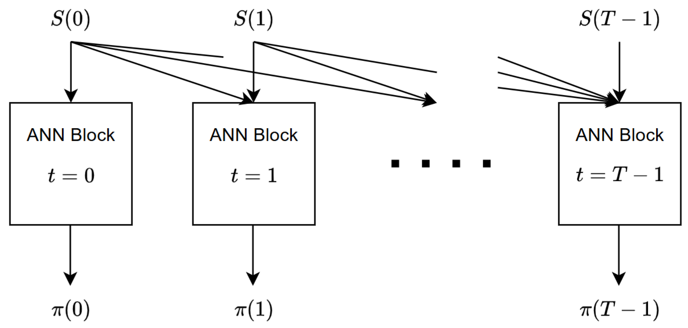
Figure 1 shows the internal structure of the ANN and its input–output flow. For each time step, we have allocated an ANN block, which is itself a multi-layer neural network. The internal structure of each ANN block will be described in Section 4. The ANN block corresponding to time step t is responsible for calculating , the portfolio weights of the time step t. The inputs to block t consist of the history of the price process up to time t, in other words, . This specific input selection is in compliance with the fact that the portfolio process should be adapted with respect to the filtration . Therefore, as can be seen in Figure 1, each price is fed to all the blocks at time t and afterwards. Regarding the input–output dimensions, block t receives a vector of dimension and returns a vector of dimension (we have dropped the batch dimensions here for simplicity). Note that we have not considered a block for , primarily due to the fact that any trading activity occurring on the final day has no impact on the portfolio’s value. Every ANN block possesses its own unique set of weights and biases, and we represent the complete array of weights and biases for all blocks as W.
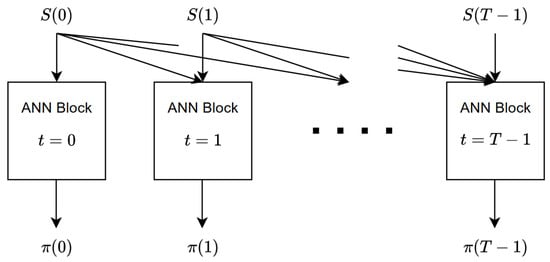
Figure 1.
The ANN, along with its inputs and outputs, consists of individual blocks assigned to each time step, with each block representing a multilayered neural network.
Now, we proceed to the calculation of the objective function of the training phase. First, we calculate the value process of the portfolio, using the recursive relation (3). Then, we calculate the final discounted value of the portfolio, . At this point, we have a tensor with dimensions , where each entry corresponds to a specific simulation of an individual parameter set. Then, we have to use (6) for calculating the expected utility of the final portfolio. The point is that we cannot calculate the exact expected value because we only have a finite sample. Therefore, we calculate an estimate of the expected value using the sample mean as follows:
We use the conventional colon notation for arrays, in which a colon means all elements of a particular dimension of the array. Here, represents a vector with elements, with each element corresponding to a distinct parameter set. We now have to take the minimum of this vector in order to obtain the following robust objective function
Here, J is the objective function that we aim to maximize. Notice that J is indeed a stochastic function, because it depends on the batch . Moreover, it obviously depends on W, the weight of the ANN. Therefore, we should denote J as . Note that the randomness of J comes solely from . Now, we can state the main problem as follows:
In this section, we formulated the robust portfolio optimization as a maximization problem over an artificial neural network. In the next section, we will implement the ANN and train it using simulated data from a stochastic model for asset prices.
4. Empirical Analysis
In this section, we evaluate the performance of the proposed algorithm through a series of analyses. First, we report the results of the algorithm applied to both simulated and real-world datasets, showcasing its effectiveness in diverse scenarios. Next, we perform a sensitivity analysis to assess the algorithm’s robustness to variations in key parameters. Finally, we compare the algorithm’s performance against a benchmark method to highlight its relative advantages and limitations. Each of these aspects is detailed in the following subsections.
4.1. Simulated Data
In this subsection, we illustrate the performance of our method on an Exponential Ornstein–Uhlenbeck (EOU) model. The EOU process is a powerful stochastic model characterized by its mean-reverting property, making it particularly advantageous for modeling dynamic systems where values tend to return to a long-term average over time. This attribute is especially pertinent in financial markets, and as a result, the EOU process has garnered extensive use as a model for asset prices. Its effectiveness stems from its capacity to account for both random fluctuations and the inherently cyclical nature of market dynamics. Additionally, the EOU process lends itself naturally to multivariate generalizations, thereby providing the flexibility required to model multiple correlated assets concurrently. This flexibility extends its utility, allowing it to capture the complex dependencies and interrelationships present in modern financial systems.
The one-dimensional Ornstein–Uhlenbeck process is described by the following Stochastic Differential Equation (SDE):
where is the speed of mean reversion, is the long-term mean, is the volatility, and is a Wiener process. To obtain the EOU process, we apply the exponential function on X to arrive at the asset price . It should be emphasized that through the application of Ito’s Lemma, it is possible to convert this SDE into an SDE specifically for the asset price. Nevertheless, due to the inclusion of exponential terms, it is more computationally efficient to utilize the mentioned SDE. Given our intention to implement the multivariate EOU process, it is essential for the parameters to be represented as matrices. In this context, is a vector with dimensionality d. This vector represents the long-term mean of the logarithm of the asset prices. Each element within the vector corresponds to the long-term mean for each asset. is a diagonal matrix of size . This matrix, often referred to as the mean reversion speed matrix, determines how quickly each asset price reverts towards its mean. is a matrix of size , where its diagonal entries represent the volatility of the logarithm of the asset prices, while the off-diagonal entries represent the covariance between various assets. Since is a symmetric matrix, the total number of parameters is .
In practice, we implement a discretized version of the EOU process in which T equally spaced time steps of the EOU process are sampled. Our simulation procedure takes the parameters of the process , the number of steps to simulate T, the number of simulations M, and the number of assets d, and generates random samples of asset prices for all d assets.
Note that although our simulations adopt an Exponential Ornstein–Uhlenbeck process, we do not fix a single parameter set for . Instead, in each training epoch, we draw a diverse set of parameters from uniform ranges, effectively capturing many plausible dynamics. This multi-parameter training procedure ensures that the learned portfolio allocations are robust against a family of possible OU models.
The generated sample paths comprised our training batch. We then fed them into the ANN to for training. The optimization method we used to train the neural network is the AMSGrad variant of adaptive moment estimation (Adam) algorithm. The Adam method calculates adaptive learning rates for each parameter, combining the advantages of other extensions of stochastic gradient descent, specifically AdaGrad and RMSProp. AMSGrad is a variant that uses the maximum of past squared gradients rather than the exponential average, which results in improved convergence properties. To generate the batch of parameters, we generated uniform random entries for the matrices .
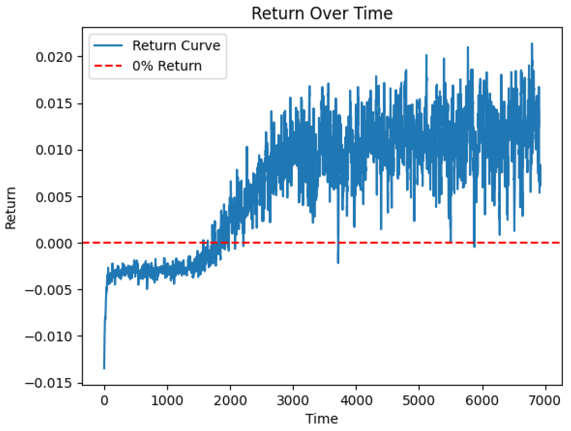
We stored the values of loss function during the training process, which is illustrated in Figure 2, showing how the robust return of the portfolio improves over training epochs.

Figure 2.
The xpected return of the portfolio under the worst-case scenario for the first 650 epochs. The plot clearly indicates that after around 350 epochs, the portfolio has a robust positive return.
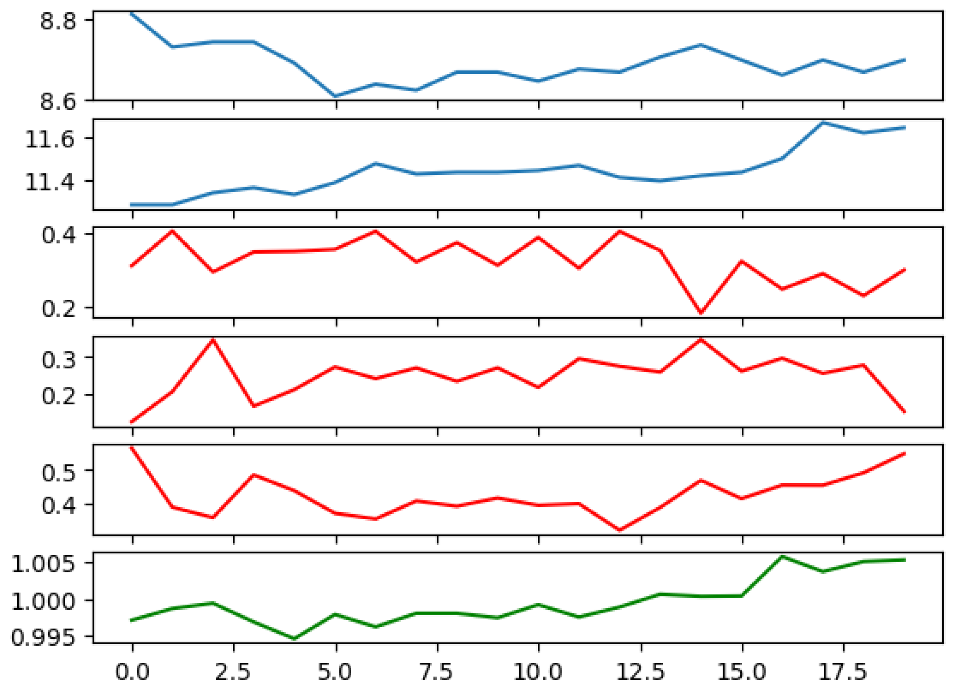
In order to elucidate the effectiveness of the ANN in learning key aspects of the financial data, we generated Figure 3, showing the prices of two risky assets over time, the calculated weights of the risky and risk-free assets assigned by the ANN, and the total value of the portfolio over time. Notably, the ANN successfully learned the mean-reverting nature of asset prices, a critical feature for predicting future asset values. An observable instance of this learning can be seen during steps 4 and 5, when the prices of both assets experience an upturn. In response, the ANN adjusts its positions, reducing holdings in these assets in anticipation of a decline in prices. This foresight embodies the network’s ability to learn from past trends and forecast future behavior.
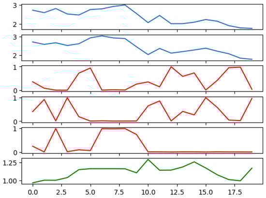
Figure 3.
Portfolio simulation result. The first two panels show the prices of two risky assets. The third, fourth, and fifth panels show the calculated weights of risky and risk-free assets. The last panel shows the total value of the portfolio. Parameters used: number of training epochs = 1000; range of parameters with ; ; ; number of risky assets = 2; number of time steps = 20; = 1000; M = 1000.
The computation times required for training our rANN model are summarized in Table 1. The times were measured under various parameter settings to demonstrate how factors such as the number of training epochs, batch size (), and number of simulations (M) affect the overall computation time. The code was executed on Google Colab, utilizing a T4 GPU runtime and 12 GB of RAM.

Table 1.
Computation time of rANN training under various parameter settings.
4.2. Real Data
We also applied our robust portfolio selection approach to real data collected from the stock market. The data set comprised the daily price values of 1145 stocks traded on the New York Stock Exchange (NYSE).
The main challenge when using real data is that unlike simulated data, there is no true value for unknown parameters. Therefore, we should accommodate the model parameter in an alternative way. To address this challenge, we consider each stock as an instantiation of a specific parameter, denoted as . Further, we regard different segments of each stock’s trajectory as simulations derived from that respective parameter. Therefore, we equate with the number of stocks in the market, and also M with the number of time segments.
In this manner, we construct a training dataset that closely mirrors our simulation experiment. Subsequently, we train the ANN utilizing this dataset. We demonstrate a sample output from the trained ANN in Figure 4.
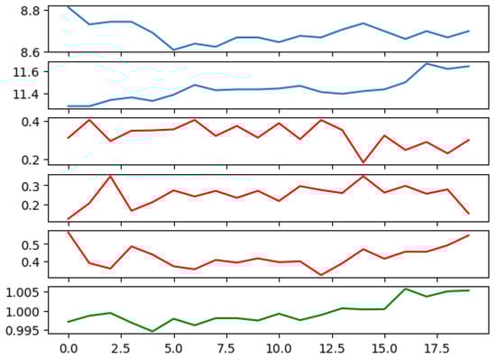
Figure 4.
A portfolio managed by the trained ANN. The first two panels depict the price of two random stocks from NYSE over an arbitrarily chosen period of 20 consecutive days. The third, fourth, and fifth panels illustrate the calculated weights of the two stocks and the risk-free asset. The last panel reveals the total value of the portfolio. Parameters used: number of training epochs = 1000; range of parameters with ; ; ; = 1000; and M = 1000.
4.3. Sensitivity Analysis
In this subsection, we discuss the influence of several key hyperparameters on the training process and the final performance of our robust portfolio selection method. Specifically, we focus on four parameters: the number of parameter samples , the number of simulated trajectories M, the risk-free rate r, and the depth of each ANN block.
First, consider , the number of parameter samples drawn from the ambiguity set in each training epoch. A larger typically provides broader coverage of the parameter space and yields a more faithful estimate of the worst-case scenario in our min-operator. However, too large a value can sharply the increase computational overhead. Conversely, too small a value can lead to an under-representation of the ambiguity set and compromise robustness.
Next, M denotes the number of simulated trajectories (or real-data segments) used per parameter. The sample mean of the final discounted value across these M trajectories approximates the expected utility. A higher M reduces variance in the gradient estimate and usually improves training stability. However, it also inflates training time. A smaller M can speed up experimentation but risks overfitting to fewer trajectories.
The hyperparameter r is the continuous risk-free rate, which appears in the discounting of the portfolio’s final value and serves as a baseline for investment returns. Higher values of r make future gains less attractive in present-value terms, often leading to more short-term strategies or higher allocations to risk-free assets. Lower values of r encourage patience and increase the relative appeal of riskier assets.
Finally, we consider the depth of each ANN block, referring to the number of hidden layers within the network that maps historical prices to portfolio weights. Deeper networks offer greater expressive power and can model more complex relationships in price data, but at the same time, they incur more computational cost.
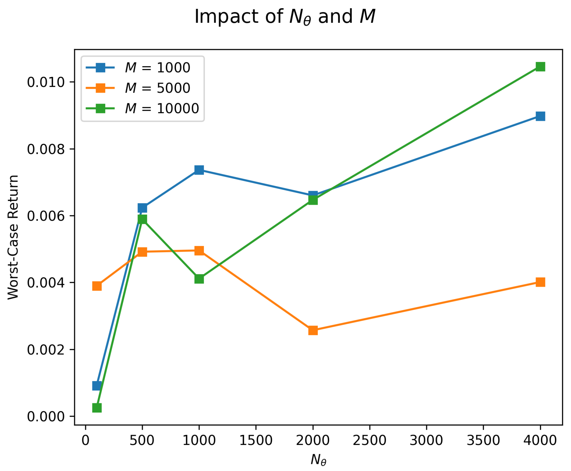
Figure 5 and Figure 6 illustrate the sensitivity of our method to these parameters by summarizing the numerical impact of varying , M, r, and network depth on the worst-case return of the portfolio. We use the same setting as that used in the numerical experiment in Section 4.1.
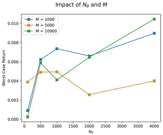
Figure 5.
How varying and M influences worst-case return.
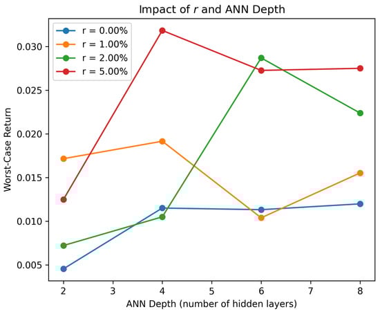
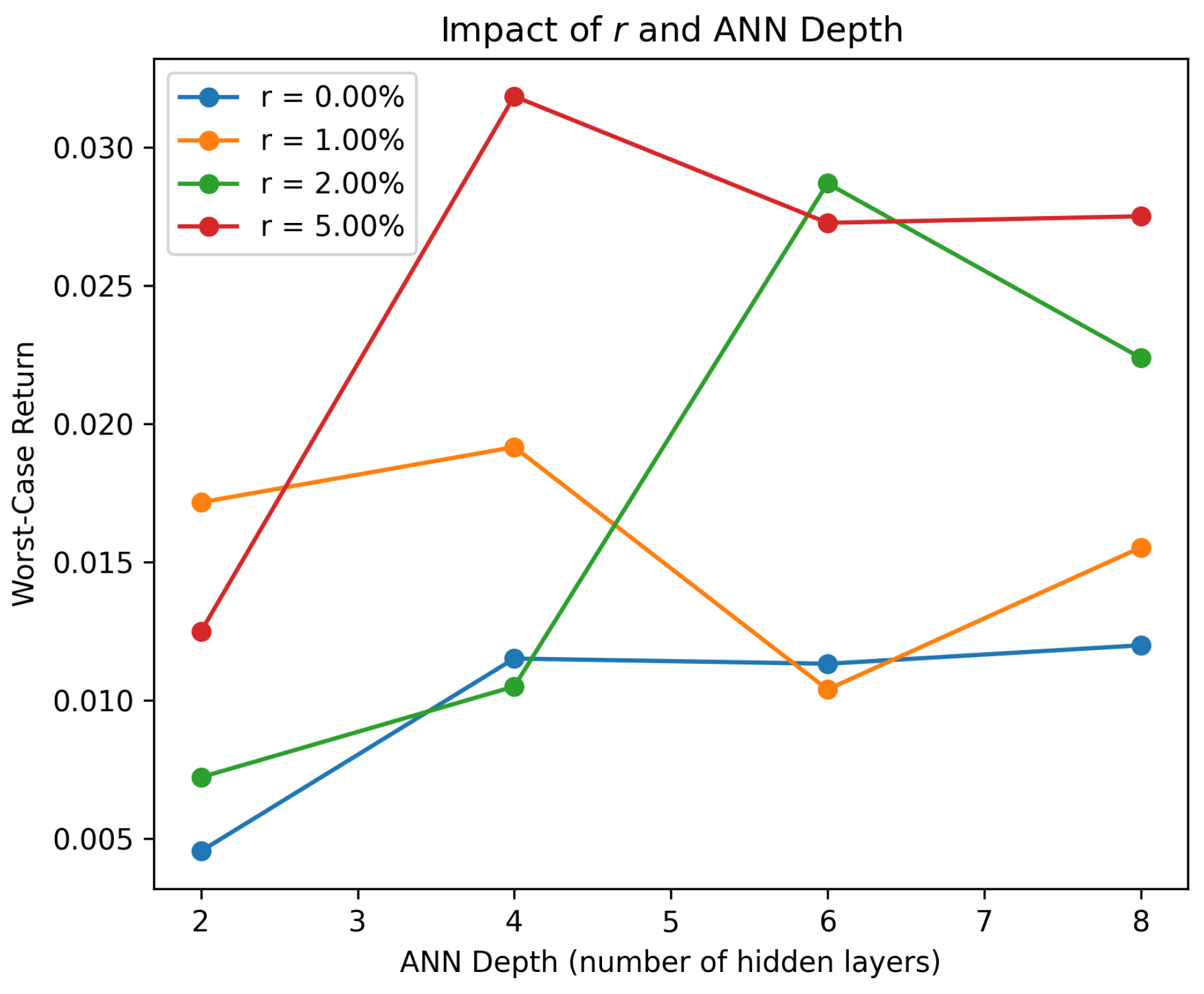
Figure 6.
The impact of different values of r and the depth of ANN blocks on the worst-case return.
In practice, these hyperparameters must be jointly optimized or tuned according to the computational budget and the desired level of robustness. Larger and M values, along with deeper networks, typically lead to stronger expressive capabilities but demand more computational resources.
4.4. Comparison to Benchmark Methods
In this subsection, we provide a comprehensive evaluation of our proposed ANN-based portfolio selection algorithm by comparing it against two benchmark methods:
- A simple equally weighted (EqW) portfolio.
- An adaptive mean–variance (AMV) approach using Exponentially Weighted Moving Average (EWMA) estimation, adapted from Guo et al. (2021).
- A Recurrent Neural Network (RNN)-based framework for portfolio optimization introduced in Cao et al. (2023).
We assess the performance of all three strategies under simulated market conditions, and then briefly discuss the results obtained from a real-world dataset.
The equally weighted portfolio allocates the same fraction of total capital to each risky asset, holding the risk-free asset only during the initial warm-up period.
We now introduce the AMV benchmark in detail. This method optimizes the portfolio weights over a given trading period, considering both a warm-up phase and a trading phase. The algorithm uses EWMA to estimate the returns and covariance matrix, which are then used in a mean–variance optimization problem. The steps of the algorithm are as follows:
- 1.
- Warm-up Period: Divide the price data into warm-up and trading periods. Hold only the risk-free asset during the warm-up period.
- 2.
- Trading Period: Iterate through the trading period , performing the following steps:
- a.
- Calculate the historical returns .
- b.
- Update the portfolio value: Based on the previous day’s returns and weights, update the portfolio value.
- c.
- Calculate the EWMA estimates: Using the historical returns up to time t, compute the exponentially weighted moving mean and covariance of the returns:where is the decay parameter of EWMA. Also, perform the EWMA calculation for the covariance matrix C,
- d.
- Portfolio Optimization: Formulate and solve the quadratic optimization problem for the weights :where b is the risk aversion parameter.
- 3.
- Calculate Performance Metrics: Compute the Sharpe ratio and maximum drawdown based on the portfolio values.
- 4.
- Tune the hyperparameters and b through grid-search cross-validation in the ranges and .
The RNN-based method of Cao et al. (2023) is designed to solve multi-objective optimization problems under time-varying parameters. The method formulates portfolio optimization as a constrained quadratic programming problem, balancing the trade-off between maximizing the expected return and minimizing risk, with transaction costs explicitly included in the constraints. The RNN is derived using a Lagrangian framework, with equality and inequality constraints enforced through projection operations and Lagrange multipliers. The network evolves dynamically to reach equilibrium, which corresponds to the optimal solution of the portfolio problem. The model is rigorously proven to exhibit global convergence and guarantees the optimality of the resulting portfolio. Furthermore, it dynamically constructs the Pareto efficient frontier by varying a trade-off parameter, enabling flexible decision-making based on risk–return preferences.
The results of the comparison include the portfolio weights for each trading day, the portfolio values over the entire trading period, the Sharpe ratio, and the maximum drawdown.
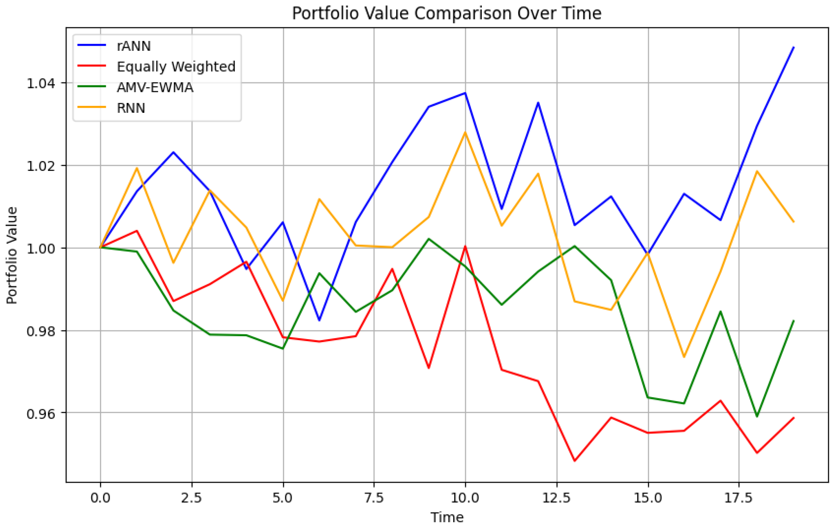
Figure 7 illustrates the cumulative growth of an initial investment of 1 unit for our ANN-based algorithm, the simple equally weighted portfolio, the AMV-EWMA algorithm, and the RNN-based algorithm. This time-series view highlights both the trend and variability in returns, allowing for a clearer comparison of the drawdowns and recoveries experienced by each approach.
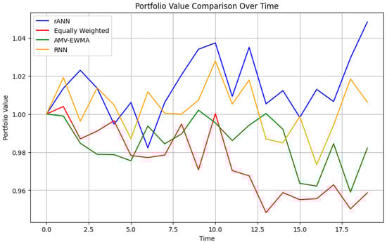
Figure 7.
Portfolio value comparison over time for the three methods: robust ANN-based method (rANN), equally weighted (EqW), AMV-EWMA, and RNN-based. The horizontal axis indicates the trading days, while the vertical axis tracks the accumulated portfolio value over time.
In this plot, the horizontal axis indicates the trading days, while the vertical axis tracks the portfolio’s accumulated value. The robust ANN-based approach shows higher cumulative returns and recovers more quickly from market drawdowns. By contrast, the AMV-EWMA strategy trails behind yet remains more adaptive than the equally weighted baseline, which displays minimal responsiveness to market shifts.
For real-world data, the superiority of the proposed rANN approach arises primarily from the following:
- Nonlinear Adaptation: Neural networks capture complex patterns and time-varying relationships in asset returns.
- Robust Feature Engineering: The inclusion of market indicators, technical factors, and macroeconomic variables can provide a more holistic representation of market conditions.
- Dynamic Allocation: Rapid rebalancing in response to changing model predictions helps limit drawdowns while seizing opportunities for enhanced returns.
The equal-weighting strategy, while providing an easily interpretable baseline, has no mechanism to adapt to changes in market conditions, whereas AMV-EWMA relies on linear mean–variance optimization, which may not fully exploit nonlinearities in the data. As a result, our ANN-based method demonstrates a clear advantage in multiple real-world scenarios.
To give a more detailed comparison of our proposed ANN-based method and the EWMA benchmark, we calculated the performance of both algorithms through metrics such as the Sharpe ratio and maximum drawdown, calculated based on the portfolio values and returns.
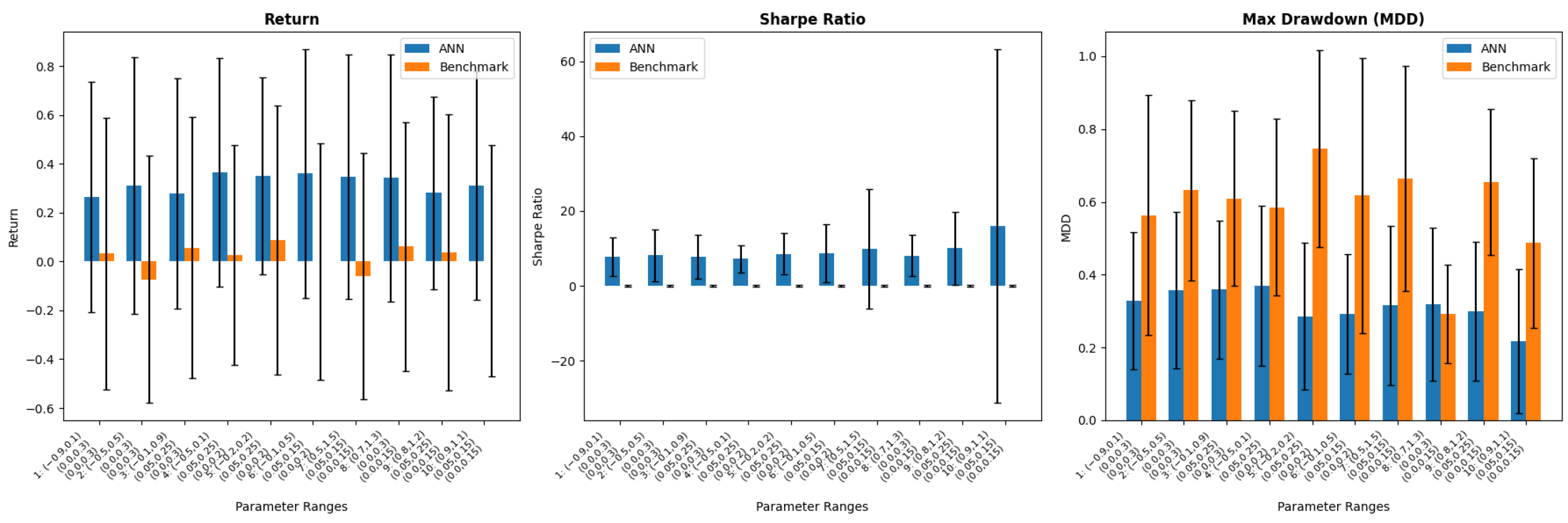
Their performance was compared over 100 simulations, and the results are shown in Table 2. Every cell within this table displays the average value across 100 simulations, accompanied by the standard deviation enclosed within parentheses. The performance values are summarized in Figure 8, demonstrating that the ANN method consistently outperforms the AMV-EWMA method in all settings and based on all three metrics considered.
Table 2.
Comparison of the ANN-based algorithm and benchmark algorithm across different parameter ranges.
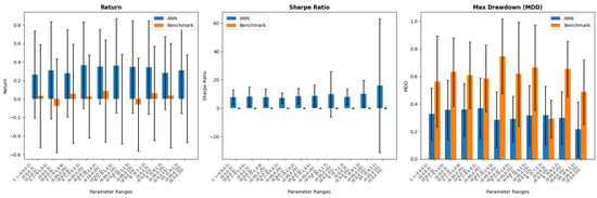
Figure 8.
Comparison of the ANN-based algorithm and AMV-EWMA across different parameter ranges.
4.5. Practical Considerations in Choosing the Ambiguity Set
In this subsection, we briefly discuss the practical aspect of choosing the ambiguity set . Incorrect specification of the ambiguity set, whether too broad or too restrictive, can lead to suboptimal portfolio performance, either by being overly cautious or by failing to account for key risks. Below are the most commonly adopted approaches and for determining in real-world contexts:
- Historical Estimation and Confidence Regions. A straightforward approach is to estimate distributional parameters (e.g., the mean vector and covariance matrix) from historical data and then form confidence regions around these estimates (Garlappi et al., 2007; Goldfarb & Iyengar, 2003). For instance, if and are the sample mean and covariance of returns, one can build an ellipsoidal ambiguity set:where is the parameter estimate from the data, is a suitable Mahalanobis distance or norm, and is chosen based on statistical confidence (e.g., a chi-square quantile). Practitioners typically select so that captures historical parameter fluctuations or prospective stress scenarios.
- Scenario-Based Intervals for Model Parameters. When a parametric family of processes (e.g., mean-reverting or factor models) is assumed, one can specify uniform or interval bounds for each parameter based on empirical ranges or expert judgment. This approach is especially common in applied financial contexts Fabozzi et al. (2007). For example, if in an Ornstein–Uhlenbeck model, the ambiguity set might beSuch interval-based approaches are often used for their simplicity, especially when historical data are limited but plausible parameter ranges are known.
- Distributionally Robust Sets (Wasserstein, , or KL Balls). An increasingly popular framework is distributionally robust optimization (DRO), where is defined as a “ball” around a nominal distribution . For example, one may use a Wasserstein ball, -ball, or Kullback–Leibler (KL) divergence ball (Blanchet & Murthy, 2019; Mohajerin Esfahani & Kuhn, 2018). A typical DRO set might bewhere D is a suitable distance (e.g., Wasserstein) and is a tolerance level. This approach accounts for uncertainty not just in the parameters (like mean and covariance) but in the entire distribution, adding another layer of robustness.
- Expert Information. In some industries, risk managers rely on expert judgment or specified stress scenarios well outside typical historical data Basel Committee on Banking Supervision (2011). One might define to encompass “worst-case” conditions or extreme shocks, such as unusually high correlation or volatility spikes. Although more subjective, this technique can be critical for capturing tail-event exposures not adequately reflected in limited samples.
In summary, there is no single best way to define , but rather, each approach chooses a trade-off between realism (capturing possible parameter variations) against tractability (avoiding unnecessarily large or overly restrictive sets). This trade-off depends on the practitioner’s risk appetite, data availability, and confidence in underlying models.
4.6. Strategies for Reducing Computational Cost
Although our proposed robust ANN-based portfolio selection method demonstrates strong performance, it can be computationally intensive. The training process, particularly for robust optimization problems, demands substantial computational resources due to the necessity of generating large training datasets through simulations, optimizing weights across multiple epochs, and evaluating the performance under diverse parameter scenarios. This computational intensity may pose a barrier for real-time applications or scenarios with limited access to high-performance computing infrastructure. Below, we summarize several strategies to mitigate these computational challenges:
- Dimensionality Reduction. Dimensionality reduction techniques, such as Principal Component Analysis (PCA) or autoencoders, can project high-dimensional financial data onto a lower-dimensional space without incurring significant information loss. By reducing input dimensionality, these methods help shorten training times and decrease memory usage (see Hinton & Salakhutdinov, 2006 for an example of autoencoders).
- Approximate or Hybrid Modeling. In cases where the exact simulation of a high-fidelity model is prohibitive, one can adopt multi-fidelity or approximate simulation techniques. For example, running a simpler (or coarser) model in early epochs and then refining it later can reduce overall computational load Peherstorfer et al. (2018).
- Hardware Optimizations and Parallelization. Modern hardware accelerators (e.g., GPUs, TPUs) can significantly speed up the simulation and training processes. Parallelizing the generation of synthetic price trajectories or real-time data preprocessing also enhances throughput Furht and Escalante (2010). Using optimized linear algebra libraries further aids in reducing runtime.
- Efficient Training Protocols. Techniques such as cyclical learning rates, warm restarts, and adaptive moment estimations (e.g., AMSGrad) can expedite network convergence and reduce the epochs needed Loshchilov and Hutter (2017). Early stopping and mini-batch training also help strike a balance between runtime and convergence quality.
- Surrogate Modeling for Parameter Space. When robust optimization requires sampling over a large set of parameters, a surrogate model can map parameter values to performance estimates Forrester et al. (2008). This makes it feasible to more efficiently identify worst-case parameter settings without exhaustive simulation across the entire ambiguity set.
5. Conclusions
We introduced a novel ANN-based framework for robust portfolio selection, focusing on parameter uncertainty in asset returns. Experiments on both simulated (Exponential Ornstein–Uhlenbeck) and real-world NYSE data showed that our approach consistently outperforms an adaptive mean–variance benchmark in terms of performance metrics like return, Sharpe ratio, and maximum drawdown. By explicitly modeling ambiguity in parameters and using simulation-based training, the ANN method offers a flexible and data-driven tool for modern portfolio management.
Nonetheless, this method relies on several assumptions and faces practical constraints. One prominent challenge lies in the computational cost associated with training artificial neural networks (ANNs). Another critical challenge involves defining the ambiguity set, which plays a central role in determining the robustness of the portfolio. The ambiguity set must balance being sufficiently comprehensive to capture the true parameter space while remaining narrow enough to avoid overly conservative or computationally intractable solutions. Also, large and high-quality datasets are required for effective neural network training, which may be impractical in data-scarce settings. Although we accommodated transaction costs, other frictions, such as liquidity constraints, were largely omitted and could affect real-world results. Additionally, the computational intensity of simulating multiple scenarios and training ANNs can pose challenges for real-time deployment.
Promising directions for future research include testing alternative risk measures and utility functions, using more advanced robust or distributionally robust optimization approaches, and incorporating realistic market frictions. Dynamic or online adaptations of our algorithm could address non-stationary market conditions more effectively. Also, improving the interpretability of ANN-based methods could help investors better understand portfolio decisions under uncertainty. Additionally, future research could explore efficient algorithmic strategies, such as transfer learning or reduced model complexity, to alleviate computational demands of our proposed method without compromising performance. Finally, while our paper adopts a parametric robustness perspective, future enhancements can incorporate fully non-parametric ambiguity sets (e.g., via moment-based or Wasserstein-based distributional sets) to align more closely with the broadest notion of distributionally robust optimization.
Author Contributions
Conceptualization, S.M. and E.S.; methodology, S.M. and E.S.; validation, S.M., E.S. and M.S.; writing—original draft preparation, S.M.; writing—review and editing, S.M., E.S. and M.S.; visualization, S.M., E.S. and M.S. All authors have read and agreed to the published version of the manuscript.
Funding
This research received no external funding.
Informed Consent Statement
Not applicable.
Data Availability Statement
The data used in this study consists of NYSE stock prices obtained from Yahoo Finance. These data are publicly available and can be accessed at https://finance.yahoo.com (accessed on 12 January 2025).
Conflicts of Interest
The authors declare no conflicts of interest.
References
- Basel Committee on Banking Supervision. (2011). Basel III: A global regulatory framework for more resilient banks and banking systems. Bank for International Settlements (BIS). [Google Scholar]
- Best, M. J., & Grauer, R. R. (1991). Sensitivity analysis for mean-variance portfolio problems. Management Science, 37(8), 980–989. [Google Scholar] [CrossRef]
- Blanchet, J., & Murthy, K. (2019). Quantifying distributional model risk via optimal transport. Mathematics of Operations Research, 44(2), 565–600. [Google Scholar] [CrossRef]
- Bradrania, R., Pirayesh Neghab, D., & Shafizadeh, M. (2022). State-dependent stock selection in index tracking: A machine learning approach. Financial Markets and Portfolio Management, 36(1), 1–28. [Google Scholar] [CrossRef]
- Cao, X., Francis, A., Pu, X., Zhang, Z., Katsikis, V., Stanimirovic, P., Brajevic, I., & Li, S. (2023). A novel recurrent neural network based online portfolio analysis for high frequency trading. Expert Systems with Applications, 233, 120934. [Google Scholar] [CrossRef]
- Chen, W., Zhang, H., Mehlawat, M. K., & Jia, L. (2021). Mean–variance portfolio optimization using machine learning-based stock price prediction. Applied Soft Computing, 100, 106943. [Google Scholar] [CrossRef]
- Cheng, T., & Chen, K. (2023). A general framework for portfolio construction based on generative models of asset returns. The Journal of Finance and Data Science, 9, 100113. [Google Scholar] [CrossRef]
- Chopra, V., & Ziemba, W. (1993). The effect of errors in means, variances, and covariances on optimal portfolio choice. Journal of Portfolio Management, 19, 6–11. [Google Scholar] [CrossRef]
- Choueifaty, Y., & Coignard, Y. (2008). Toward maximum diversification. Journal of Portfolio Management, 35, 40–51. [Google Scholar] [CrossRef]
- Cont, R., & Nitions, D. (1999). Statistical properties of financial time series. In Mathematical finance: Theory and practice. Lecture series in applied mathematics. Higher Education Press. [Google Scholar]
- Fabozzi, F. J., Kolm, P. N., Pachamanova, D. A., & Focardi, S. M. (2007). Robust portfolio optimization and management. John Wiley & Sons. [Google Scholar]
- Fernholz, E. R., & Fernholz, E. R. (2002). Stochastic portfolio theory. Springer. [Google Scholar]
- Forrester, A., Sobester, A., & Keane, A. (2008). Engineering design via surrogate modelling: A practical guide. John Wiley & Sons. [Google Scholar]
- Furht, B., & Escalante, A. (Eds.). (2010). Handbook of cloud computing. Springer. [Google Scholar]
- Garlappi, L., Uppal, R., & Wang, T. (2007). Portfolio selection with parameter and model uncertainty: A multi-prior approach. The Review of Financial Studies, 20(1), 41–81. [Google Scholar] [CrossRef]
- Goldfarb, D., & Iyengar, G. (2003). Robust portfolio selection problems. Mathematics of Operations Research, 28(1), 1–38. [Google Scholar] [CrossRef]
- Goodfellow, I., Bengio, Y., & Courville, A. (2016). Deep learning. MIT Press. Available online: https://books.google.com/books?id=Np9SDQAAQBAJ (accessed on 12 January 2025).
- Guo, S., Gu, J.-W., & Ching, W.-K. (2021). Adaptive online portfolio selection with transaction costs. European Journal of Operational Research, 295(3), 1074–1086. [Google Scholar] [CrossRef]
- Hinton, G. E., & Salakhutdinov, R. R. (2006). Reducing the dimensionality of data with neural networks. Science, 313(5786), 504–507. [Google Scholar] [CrossRef] [PubMed]
- Ismail, A., & Pham, H. (2019). Robust Markowitz mean-variance portfolio selection under ambiguous covariance matrix. Mathematical Finance, 29(1), 174–207. [Google Scholar] [CrossRef]
- Kang, Z., Li, X., Li, Z., & Zhu, S. (2019). Data-driven robust mean-CVaR portfolio selection under distribution ambiguity. Quantitative Finance, 19(1), 105–121. [Google Scholar] [CrossRef]
- Karatzas, I., & Fernholz, R. (2009). Stochastic portfolio theory: An overview. Handbook of Numerical Analysis, 15, 89–167. [Google Scholar]
- LeCun, Y., Bengio, Y., & Hinton, G. (2015). Deep learning. Nature, 521, 436–444. [Google Scholar] [CrossRef]
- Loshchilov, I., & Hutter, F. (2017, April 25–29). SGDR: Stochastic gradient descent with warm restarts. Proceedings of the International Conference on Learning Representations (ICLR), Virtual Event. [Google Scholar]
- Lotfi, S., & Zenios, S. A. (2018). Robust VaR and CVaR optimization under joint ambiguity in distributions, means, and covariances. European Journal of Operational Research, 269(2), 556–576. [Google Scholar] [CrossRef]
- Markowitz, H. (1952). Portfolio selection. The Journal of Finance, 7(1), 77–91. Available online: http://www.jstor.org/stable/2975974 (accessed on 12 January 2025).
- Min, L., Dong, J., Liu, J., & Gong, X. (2021). Robust mean-risk portfolio optimization using machine learning-based trade-off parameter. Applied Soft Computing, 113, 107948. [Google Scholar] [CrossRef]
- Mohajerin Esfahani, P., & Kuhn, D. (2018). Data-driven distributionally robust optimization using the Wasserstein metric: Performance guarantees and tractable reformulations. Mathematical Programming, 171(1), 115–166. [Google Scholar] [CrossRef]
- Peherstorfer, B., Willcox, K., & Gunzburger, M. (2018). Survey of multifidelity methods in uncertainty propagation, inference, and optimization. SIAM Review, 60(3), 550–591. [Google Scholar] [CrossRef]
- Tsang, K. H., & Wong, H. Y. (2020). Deep-learning solution to portfolio selection with serially dependent returns. SIAM Journal on Financial Mathematics, 11(2), 593–619. [Google Scholar] [CrossRef]
- Wild, R. (2008). Index investing for dummies. John Wiley & Sons. [Google Scholar]
- Wu, Z., & Sun, K. (2023). Distributionally robust optimization with Wasserstein metric for multi-period portfolio selection under uncertainty. Applied Mathematical Modelling, 117, 513–528. [Google Scholar] [CrossRef]
- Xidonas, P., Steuer, R., & Hassapis, C. (2020). Robust portfolio optimization: A categorized bibliographic review. Annals of Operations Research, 292(1), 533–552. [Google Scholar] [CrossRef]
- Zhang, Z., Zohren, S., & Roberts, S. (2019). Extending deep learning models for limit order books to quantile regression. arXiv, arXiv:1906.04404. [Google Scholar]
- Zhang, Z., Zohren, S., & Roberts, S. (2020). Deep learning for portfolio optimization. The Journal of Financial Data Science, 2(4), 8–20. [Google Scholar] [CrossRef]

Disclaimer/Publisher’s Note: The statements, opinions and data contained in all publications are solely those of the individual author(s) and contributor(s) and not of MDPI and/or the editor(s). MDPI and/or the editor(s) disclaim responsibility for any injury to people or property resulting from any ideas, methods, instructions or products referred to in the content. |
© 2025 by the authors. Licensee MDPI, Basel, Switzerland. This article is an open access article distributed under the terms and conditions of the Creative Commons Attribution (CC BY) license (https://creativecommons.org/licenses/by/4.0/).