Article

A Hybrid of Box-Jenkins ARIMA Model and Neural Networks for Forecasting South African Crude Oil Prices

by
Johannes Tshepiso Tsoku
*,
Daniel Metsileng
and
Tshegofatso Botlhoko
Department of Business Statistics and Operations Research, North-West University, Mafikeng Campus, Mmabatho 2745, South Africa
*
Author to whom correspondence should be addressed.
Int. J. Financial Stud. 2024, 12(4), 118; https://doi.org/10.3390/ijfs12040118
Submission received: 22 September 2024 / Revised: 15 November 2024 / Accepted: 24 November 2024 / Published: 28 November 2024

Abstract

:
The current study aims to model the South African crude oil prices using the hybrid of Box-Jenkins autoregressive integrated moving average (ARIMA) and Neural Networks (NNs). This study introduces a hybrid approach to forecasting methods aimed at resolving the issues of lack of precision in forecasting. The proposed methodology includes two models, namely, hybridisation of ARIMA with artificial neural network (ANN)-based Extreme Learning Machine (ELM) and ARIMA with general regression neural network (GRNN) to model both linear and nonlinear simultaneously. The models were compared with the base ARIMA model. The study utilised monthly time series data spanning from January 2021 to March 2023. The formal stationarity test confirmed that the crude oil price series is integrated of order one, I(1). For the linear process, the ARIMA (2,1,2) model was identified as the best fit for the series and successfully passed all diagnostic tests. The ARIMA-ANN-based ELM hybrid model outperformed both the individual ARIMA model and the ARIMA-GRNN hybrid. However, the ARIMA model also showed better performance than the ARIMA-GRNN hybrid, highlighting its strong competitiveness compared to the ARIMA-ANN-based ELM model. The hybrid models are recommended for use by policy makers and practitioners in general.

1. Introduction

Accurate forecasting of crude oil prices is vital for energy organisations, policy makers, and partners in the oil business. Accurate oil price forecasting is crucial for policy makers when developing economic plans, energy regulations, and even diplomatic initiatives. National economies can be greatly impacted by changes in oil prices, particularly those that depend largely on oil imports or exports. Governments may prepare for energy security and sustainability by using forecasting models to predict changes in inflation, trade balances, and tax revenues. Additionally, it assists them in assessing how any policy changes, such as carbon taxes, subsidies, or regulations, will affect the production and use of oil. South Africa, as a huge oil shipper, is especially defenceless against fluctuations in worldwide unrefined petroleum costs. Time series prediction is highly significant across a range of fields, including stock prices, industrial planning, currency exchange rates, water usage, healthcare, and the consumer price index, among others. Conventional time series models, like autoregressive integrated moving average (ARIMA), have been broadly utilised for oil cost determining yet frequently struggle to capture nonlinear relationships and complexities. In the meantime, Neural Networks (NNs) have shown guarantee in demonstrating complicated designs yet can be restricted by their dependence on enormous datasets. According to Goswami and Kandali (2020) and Wang et al. (2012), early methods for time series forecasting depended solely on statistical techniques, such as regression analyses, ARIMA, and many others. These statistical methods are effective for data with linear relationships. For nonlinear data, however, artificial intelligence (AI) models, particularly NNs, have been developed (Shao et al. 2017; Zheng et al. 2017). Recently, hybrid methods that integrate statistical techniques with deep learning approaches have been developed to achieve more accurate predictions (Shelatkar et al. 2020; Wu et al. 2021).
This study aims to evaluate the effectiveness of hybrid models that combine ARIMA with general regression neural network (GRNN) and artificial neural network (ANN)-based Extreme Learning Machine (ELM) for forecasting South African crude oil prices. By training and assessing these models with historical price data, the study seeks to gauge their accuracy and reliability in predicting future price movements. It is among the few studies to apply advanced machine learning (ML) methods (GRNN and ANN-based ELM) alongside ARIMA models to explore forecasting performance for South African crude oil prices. These methods, which employ ANNs and evolutionary algorithms rather than traditional time series models, can uncover nonlinear relationships and patterns in oil price data, resulting in more accurate and reliable predictions. This study contributes to existing knowledge by demonstrating the effectiveness of combining ARIMA with neural network (NN) models for predicting crude oil performance. Additionally, the study provides an in-depth analysis of the forecasting abilities of these models concerning South African crude oil prices. It also advances current knowledge by illustrating how combining ML with traditional/conventional approaches can address the uncertainties and complexities of oil price predictions, thereby helping the energy sector make more informed decisions.
The capacity of ARIMA, GRNN, and ANN-ELM to handle time series data makes them ideal choices over other forecasting techniques like Random Forest, Gradient Boosting, Support Vector Machine (SVM), Naïve Bayes, and k-nearest neighbors (KNN). ARIMA, with its ability to model temporal relationships, trends, and seasonality in stationary data, is particularly well-suited for time series forecasting (Box et al. 2015). When the data exhibit complex patterns that linear models like ARIMA cannot capture, GRNN becomes the method of choice due to its ability to handle noisy data and model intricate, nonlinear relationships (Specht 1991). ANN-ELM models, known for their fast-training times and high generalisation performance, are preferred when dealing with large and complex datasets (Huang et al. 2004). According Breiman (2001), Chen and Guestrin (2016), and Vapnik (2013) methods like Random Forest, Gradient Boosting, SVM, Naïve Bayes, and KNN, while effective in various contexts, do not inherently account for the temporal dependencies in time series data, making ARIMA, GRNN, and ANN-ELM more appropriate for accurate and efficient forecasting tasks.
This study proposes a novel hybrid approach, consolidating the qualities of Box-Jenkins ARIMA models and NNs to model South African crude oil prices. By incorporating the robustness of ARIMA with the versatility of NNs, this crossover model intends to work on the precision and dependability of crude oil price expectations. The paper investigates the capability of this imaginative way to deal with addressing the difficulties of crude oil prices, giving important bits of knowledge to partners in the energy area. The partitioning of the data provides a unique perspective by focusing on the different periods (pre-, during-, and post-COVID-19), which introduces variations compared to the overall sample. It was evident that ARIMA outperformed the hybrid models across the different partitions.
The remainder of the paper is organised as follows: Section 2 provides the literature review, Section 3 outlines the methodology, Section 4 discusses the findings, and Section 5 offers the conclusion and recommendations.

2. Literature Review

Yu et al. (2020) conducted a comparison of different techniques, including the EWT technique, Artificial Bee Colony (ABC) algorithm, ELM neural network (NN), and ARIMA linear algorithm to forecast NAIRA stock prices. The findings highlighted the remarkable capabilities of the proposed algorithm in parameter optimisation. The optimised ELM model demonstrated superior performance over the original ELM, ABC-ELM, long short-term memory (LSTM), and ANN models, particularly in terms of stability and precision. As a result, it exhibited superior performance in financial time series forecasting compared to other models. The study by Al-Gounmeein and Ismail (2021) compared the effectiveness of ANN models combined with autoregressive fractionally integrated moving average (ARFIMA) models in forecasting Brent crude oil prices. Their hybrid approach, which integrated ARFIMA with multilayer perceptron (MLP), demonstrated superior performance compared to both the individual models and other hybrid models.
In a separate study, Aggarwal et al. (2023) used ARIMA and ANN models to forecast major electricity markets. They found that the ARIMA models, specifically ARIMA (2,1,2) and ARIMA (3,1,3), were most appropriate for modelling natural gas (NG) and coal, respectively. The best ANN models for coal and NG were NNAR (31,16) and NNAR (10,6), respectively. The results indicated that ANN was the most robust model for forecasting both commodities.
The study by Karimuzzaman et al. (2020) aimed to assess effective models for diagnosing positive COVID-19 cases in Telangana State, India. The study incorporated the ELM, MLP, LSTM, and ARIMA models. Data spanning from 1st December 2020 to 30th May 2021 were analysed. The results revealed the LSTM model as the most efficient, with the lowest Root Mean Square Error (RMSE = 71.12), surpassing the ARIMA (258.20), ELM (553.67), and MLP (641.86) models. This underscores the LSTM model’s effectiveness in accurately predicting COVID-19 cases, offering valuable insights for public health management in Telangana State, ()India.
Cihan (2024) evaluated the effectiveness of deep learning, traditional, and hybrid time series models for forecasting ecological footprints (EF). The study involved using deep learning techniques like LSTMs, classical series models such as ARIMA and Holt-Winters, and a hybrid ARIMA-SVR model. The results indicated that the ARIMA (1,1,0) model outperformed the Holt-Winters, LSTM, and ARIMA-SVR models on the test dataset.
In another study, Buliali et al. (2016) conducted a study on GRNN for Predicting Traffic Flow. The study compared the GRNN results to other forecasting methods such as ARIMA, Single Exponential Smoothing, Moving Average, and Leave One Out Cross Validation (LOOCV) to test the traffic flow data. The study used Mean Absolute Percentage Error (MAPE) as the evaluation criterion. The study used traffic flow data obtained from the Traffic Highway Agency in England. The results of the study revealed that the GRNN method outperformed ARIMA, Single Exponential Smoothing, and Moving Average in predicting traffic flow data, as it reduced the MAPE. Buliali et al. (2016) concluded that the GRNN model was well-suited for forecasting traffic flow data, which was often dynamic and nonlinear in nature.
Jagan et al. (2019) investigated reliability analysis to assess the safety of simply supported beams under uniformly distributed loads. The analysis incorporated datasets containing Modulus of Elasticity (E), Load intensity (w), and performance function (δ), where E and W were utilised as inputs and δ as the output. The study employed GRNN, ELM, and GPR models. The results indicated the superiority of the GRNN model over ELM and GPR models in reliability assessment. Additionally, the Coefficient of Determination (R2) achieved 0.998 for training and 0.989 for testing, demonstrating the efficacy of the model in capturing the relationship between inputs and outputs.
The study by Feng et al. (2017) employed ELM, Backpropagation NNs optimised by Genetic Algorithm (GANN), Random Forests (RF), and GRNN to estimate daily diffuse solar radiation (Hd) at two meteorological stations in the North China Plain (NCP). The results revealed that all four models outperformed the empirical Iqbal model in estimating daily Hd. Despite underestimating Hd for both stations, the AI models exhibited average relative errors ranging from −5.8% to −5.4%, whereas the Iqbal model showed a higher average relative error of 19.1% in Beijing and −5.9% to −4.3% and −26.9% in Zhengzhou. Among the AI models, the GANN model demonstrated the highest accuracy, followed by ELM, RF, and GRNN models. Although the ELM model exhibited slightly poorer performance, it boasted the highest computation speed. Both the GANN and ELM models are recommended for estimating daily Hd in the NCP of China.
Sha et al. (2019) modelled and predicted the railway passenger flow using the hybrid of ARIMA and ELM. The findings of the study revealed that the prediction accuracy of the proposed hybrid model is higher than the one for the ARIMA, ELM, or seasonal model when computed individually. The study proved the effectiveness and superiority of the hybrid model proposed. In another study, Peng et al. (2021) predicted the stock index using a hybrid ARIMA-ELM model. The study used the Shanghai Composite 50 Index as the target for simulation experiments. Using the root mean square error (RMSE) and MAE, the results of the simulation experiments indicated that the hybrid model outperformed both the individual ARIMA model and the ELM model, demonstrating superior predictive performance.
Similarly, the study by Moseane et al. (2024) examined the Johannesburg Stock Exchange/Financial Times Stock Exchange (JSE/FTSE) closing stock prices using the hybrid of time series and ANN-based ELM models. The models used in the study were ARIMA, ANN-based ELM, and the hybrid of ARIMA-ANN-based ELM. The error metrics showed that the hybrid ARIMA-ANN-based ELM model outperformed both the ARIMA model and the ANN-based ELM model individually.
Wei et al. (2017) conducted a study on a hybrid of ARIMA and GRNN for the incidence of Tuberculosis in Heng County, China. Four models were employed to fit and predict the incidence of tuberculosis: the ARIMA model, a traditional ARIMA–GRNN hybrid model, a basic GRNN model, and a novel ARIMA–GRNN hybrid model. Using mean absolute error (MAE), mean absolute percentage error (MAPE), and mean square error (MSE), the study found that the new ARIMA–GRNN model demonstrated a better fit compared to both the traditional ARIMA–GRNN model and the basic ARIMA model, both when applied to historical data and when used for forecasting incidence over the following 6 months. Similarly, the study by Bărbulescu et al. (2022) also found that hybrid ARIMA-GRNN was the best fit model when compared with ARIMA and GRNN individually. In addition, according to the study by Li et al. (2019), the ARIMA-GRNN hybrid model proved to be more effective than the single ARIMA model in predicting short-term tuberculosis incidence in the Chinese population, particularly in accurately fitting and forecasting the peak and trough of incidence rates.

3. Methodology

The paper utilised monthly time series data from January 2000 to November 2023, with observations sourced from the South African Reserve Bank. The data are publicly available and can be accessed at http://www.resbank.co.za (accessed on 26 March 2024). ARIMA, GRNN, and ANN-based ELM have been used individually in different studies to model the linear and nonlinear characteristics of the time series data. However, none of these models are universally applicable to all scenarios. The paper suggested employing linear and nonlinear methods simultaneously to form a hybrid to model the crude oil prices. The dataset was split into two subsets, namely, 80% for training and 20% for testing. Data analysis was conducted using Python software version 2022.3.3, and the details of the models are discussed in the following subsections.

3.1. ARIMA Model

For the past thirty years, ARIMA models have been a dominant choice in various fields of time series forecasting. Developed by Box and Jenkins in the early 1970s, the ARIMA model is a well-established method for predicting time series data (Jenkins and Box 1976). The general form of ARIMA (p,d,q) is given by:
φ p ( B ) ( 1 B ) d y t μ = θ q ( B ) ε t
where φ p B = 1 i = 1 p φ i B i ,   θ q B = 1 j = 1 q θ j B j are polynomials in terms of B of degree of freedom p and q ,   r e s p e c t i v e l y ,   = ( 1 B ) and B is the backward shift operator. The Box-Jenkins approach consists of four iterative stages: model identification, parameter estimation, diagnostic testing, and evaluation of the forecasting model. During the first step, data transforming is necessary to achieve stationarity, a prerequisite for constructing an ARIMA (p,d,q) model. Dickey and Fuller (1979) pioneered stationarity testing, which they described as “testing for a unit root”, as detailed by Tsoku et al. (2017). They introduced the Augmented Dickey–Fuller (ADF) test as a formal method to evaluate the presence of a unit root. Later, in 1992, the Kwiatkowski–Phillips–Schmidt–Shin (KPSS) test, developed by Kwiatkowski, Phillips, Schmidt, and Shin, was introduced as a complementary or alternative approach to the ADF test (Kwiatkowski et al. 1992). This paper employs both the ADF and KPSS tests to assess stationarity in the time series data. Once the training and testing datasets are fully prepared, they are processed to reduce data noise, such as white noise and non-stationarity, using techniques such as the Autocorrelation Function (ACF) and Partial Autocorrelation Function (PACF).

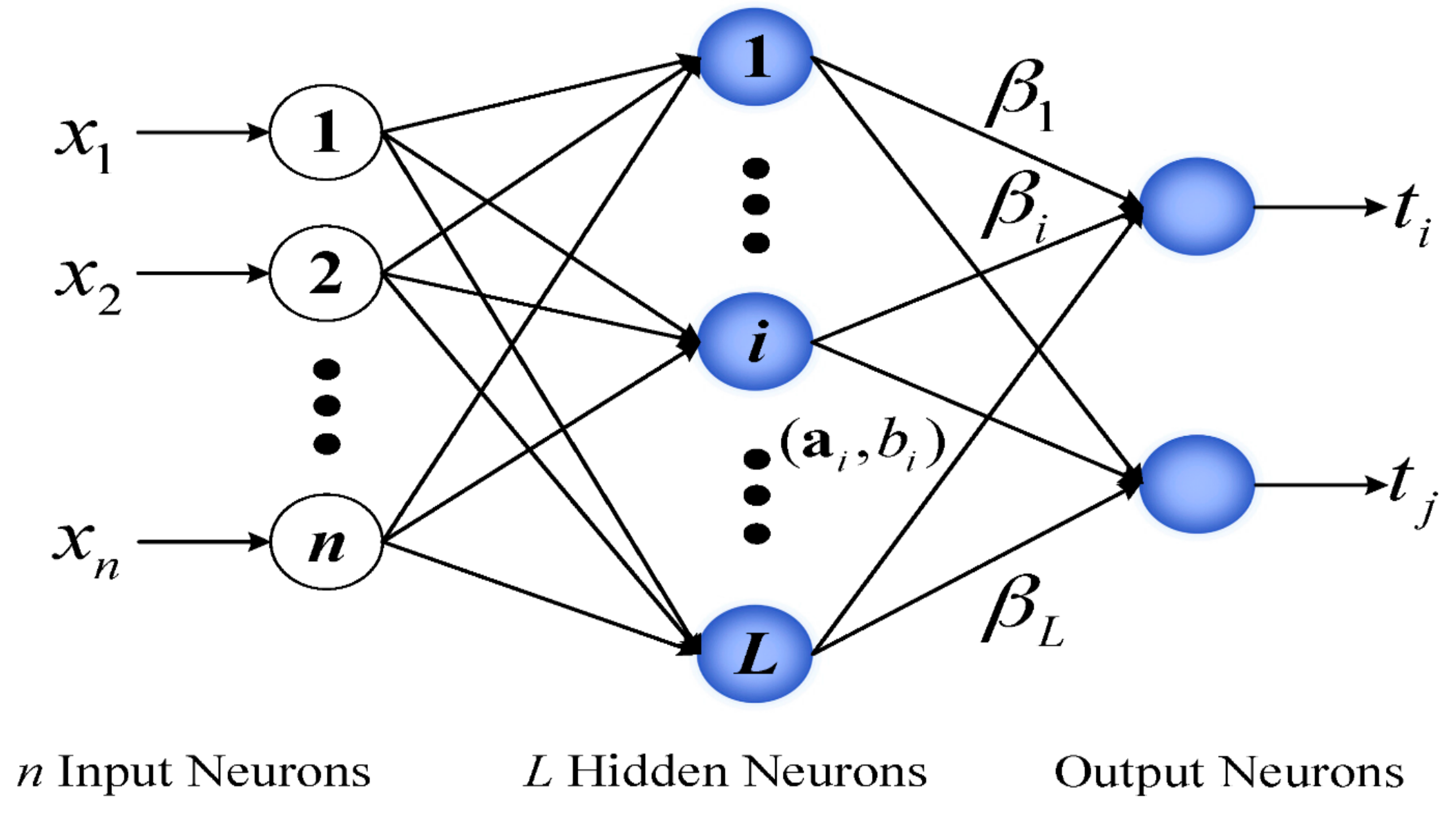
3.2. Hybridisation of ARIMA-ANN-Based ELM

The ARIMA model is integrated with the ANN-based ELM model by using the residuals from the ARIMA model to determine the weights for the ANN-based ELM model. These weights are then used to assess the forecasting performance of the model (Singh and Balasundaram 2007; Siripanich et al. 2007; Wang and Hu 2015). In this proposed approach, the input weights and hidden biases for the ARIMA model are assigned randomly, while the output weights are computed analytically using the Moore–Penrose (MP) generalised inverse method. Given a training dataset with N unique samples ( x i ,   t i ) R n × R m , the output of the Single-Layer Feedforward Network (SLFN) with N ^ hidden neurons and zero error can be expressed as:
i = 1 N ^ β i g ( w i ,   x j , b i ) = t j ,   j = 1 ,   2 ,   ,   N
where w i represents the input weights, β i denotes the weights connecting the hidden layer to the output layer, and b i are the biases in the hidden layer. The matrix representation of the N equations in Equation (2) is given by:
= T
where
H = g ( w 1 ,   x 1 , b 1 ) g ( w L ,   x 1 , b L ) g ( w 1 ,   x N , b 1 ) g ( w L ,   x N , b L ) N × N ^ ,   β = β 1 β 2 β L N ^ × m   and   T = t 1 t 2 t N N × m
Due to the random assignment of weights w i and biases b i , the weight vector β is the only unknown parameter that needs to be estimated. However, because the arrangement of the output weight matrix H of the hidden layer can vary depending on the data sample and the number of hidden neurons N ^ , Equation (3) may not always be consistent. Therefore, estimating β essentially becomes the least squares optimisation problem in the following form:
Ω β = m i n H β T 2 2
Chong and Żak (2013) stated that, according to optimisation theory, the solution that minimises the objective function Ω β is given by:
β = H T
where H = ( H T H ) 1 H T is the MP generalised inverse (also called the pseudo-inverse) of H . The key difference between ELM and traditional neural network methods is that ELM does not require fine-tuning of all the parameters of the feedforward network, including input weights and hidden layer biases. Figure 1 illustrates the schematic structure of ELM:

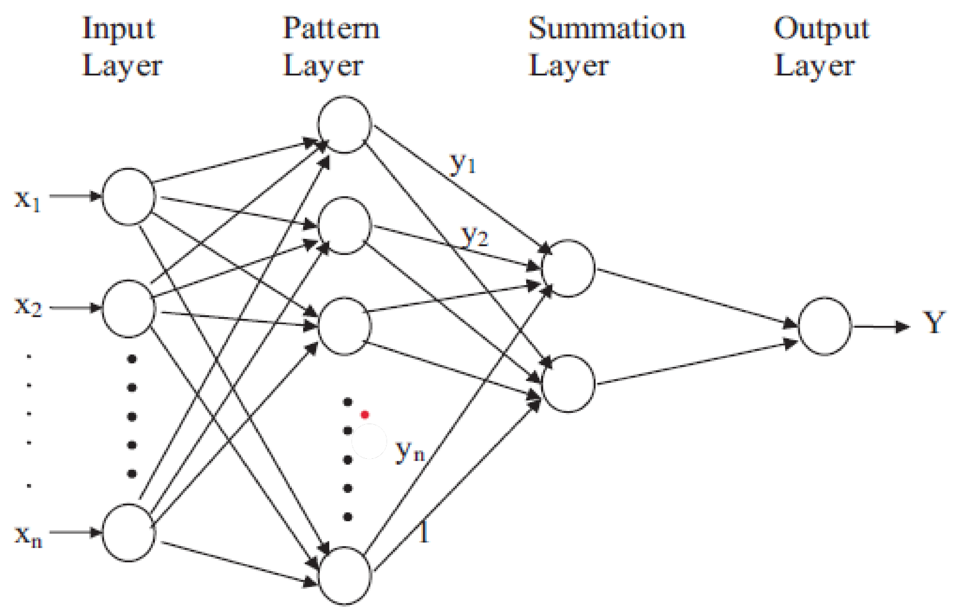
3.3. Hybridisation of ARIMA-GRNN

In the hybrid ARIMA-GRNN approach, an ARIMA model is first developed for the original data series, and subsequently, the residuals from the ARIMA model are modelled using a GRNN. The GRNN was first introduced by Specht in 1991 and provides several advantages as a meta-modelling algorithm (Specht 1991). As noted by Hu et al. (2017), the GRNN is based on non-parametric regression principles and operates on sampled data using Parzen non-parametric estimation. It determines network output through the maximum probability principle and does not need an iterative training process like the backpropagation method. Compared to other networks, the GRNN model excels in nonlinear mapping and demonstrates strong learning capabilities (Wei et al. 2017).
According to Kim et al. (2004), a GRNN consists of four layers: input, pattern, summation, and output. The input layer receives data through various observed parameters corresponding to the input units. The pattern layer holds the training patterns, while the summation layer contains two types of neurons: single-division neurons, which are linked to the pattern layer, and summation neurons, which are connected to the output layer. Radial basis functions and linear activation functions are used in the hidden and output layers, respectively. Finally, the output layer normalises the results by dividing the output of each S-summation neuron by the output of each D-summation neuron, thereby generating the predicted value Y i for the unknown input vector x given as:
Y i = i = 1 n y i . e x p D ( x , x i ) i = 1 n e x p D ( x , x i )
where
D x , x i = k = 1 m x i x i k σ 2
In this context, n represents the number of training patterns, and y i denotes the weighted connection between the ith pattern layer neuron and the S-summation neuron. The Gaussian function is represented by D , m is the number of elements in the input vector, and x k , and x i k are the jth elements of x and x i , respectively. The optimal value for the spread parameter, denoted by σ , is determined through experimentation. The schematic diagram of a GRNN architecture is summarised in Figure 2.

3.4. Assessment of the Models’ Forecasting Performance

In this study, evaluation metrics are used to assess the performance of the proposed models. These metrics include the Root Mean Square Error (RMSE) and the Mean Absolute Error (MAE). The metrics are computed using the following equations:
R M S E = 1 N i = 1 N y i y ^ i 2
M A E = 1 n i = 1 N y i y ^ i
where y i represents the actual crude oil prices and y ^ i denotes the predicted crude oil prices, with N being the total number of observations.

4. Discussion of Findings

This section provides an analysis of the study’s findings. The results are displayed in tables and figures.

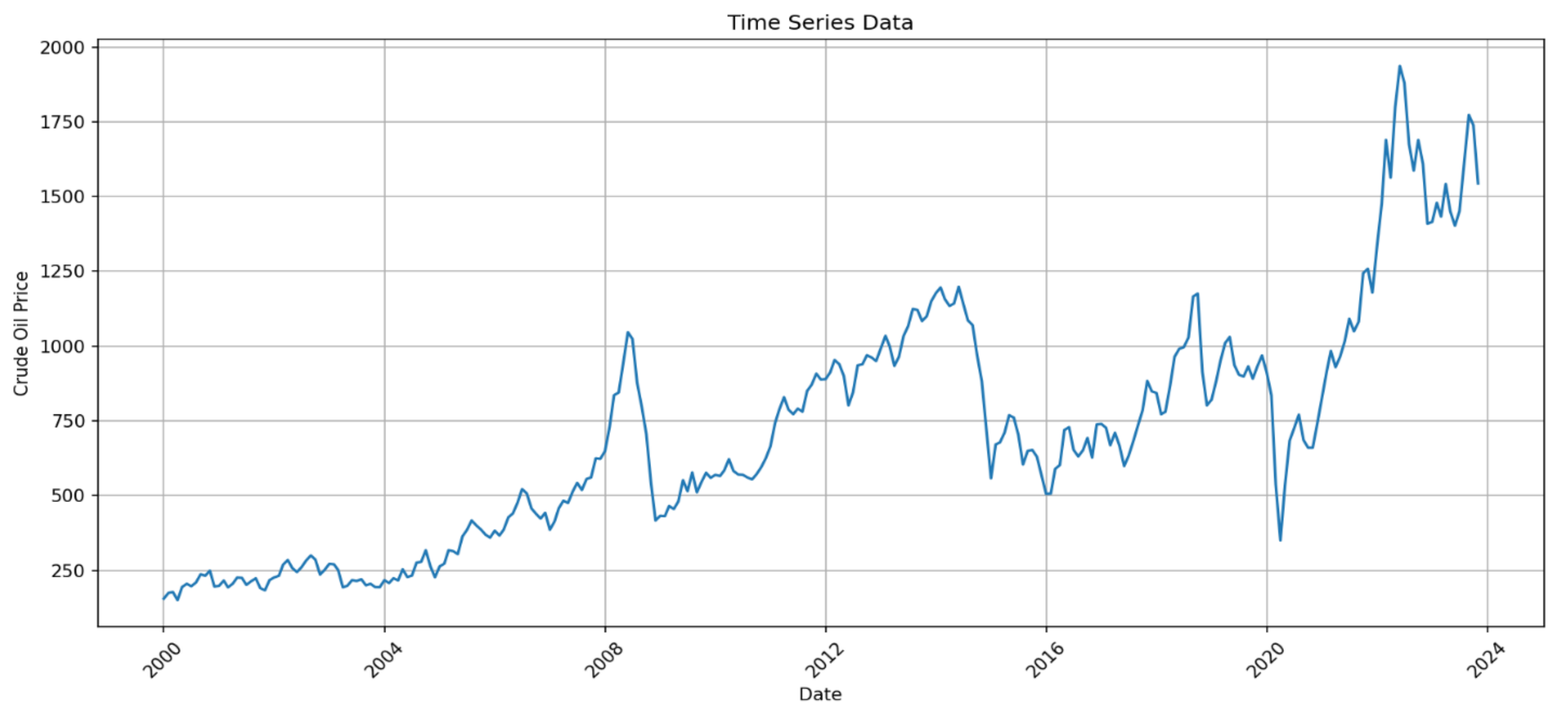
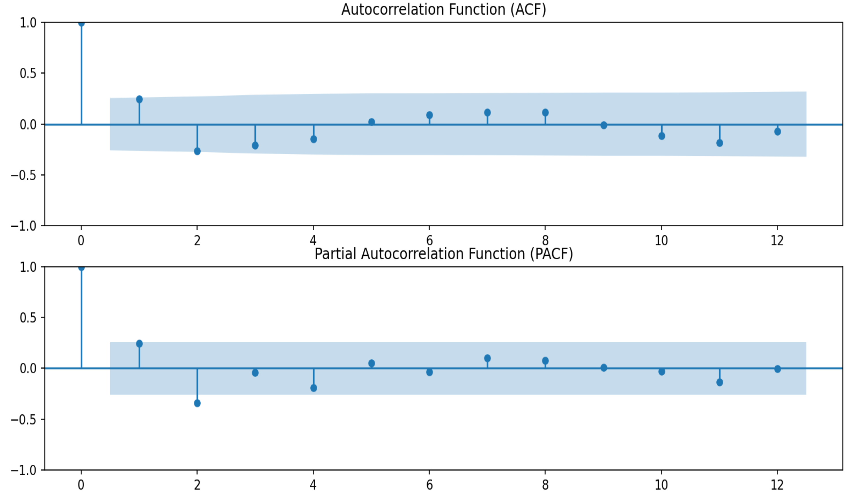
4.1. Exploratory Data Analysis (EDA)

Exploratory data analysis was conducted to grasp the characteristics of the dataset, with the findings displayed in Table 1.
The crude oil price dataset contains 287 observations, with an average price of 702.651, suggesting that prices generally hover around this value. However, the median price is 660.490, which is lower than the mean, indicating a positive skew in the distribution where higher values are inflating the average. The most common price is 416.890, significantly lower than both the mean and median, suggesting that lower prices are more frequent. The high variance of 154,137.133 and standard deviation of 392.603 reflect a substantial variability in the prices, showing a wide spread around the average. Prices range from a minimum of 150.470 to a maximum of 1936.560, highlighting the significant volatility and dispersion within the dataset. Figure 3 provides a visual representation of the crude oil prices.
As shown in Figure 3, the crude oil price plot appears to be nonstationary, exhibiting noticeable fluctuations over the sample period. Significant spikes occurred around 2006, 2010, and late 2022, indicating periods of substantial volatility in crude oil prices. Visual inspection suggests that the series is nonstationary. To confirm this, a formal stationarity test was conducted, with the results detailed in Table 2.
The results in Table 2 show that the p-value of the ADF test is 0.685, which is much higher than the 0.05 significance level, indicating non-stationarity at the level. Conversely, the KPSS test yields a p-value of 0.01, which is below the 0.05 threshold, also suggesting non-stationarity. These findings align with the visual assessment of the series, confirming that the data are non-stationary at level and require differencing for stationarity. After differencing the series, the p-value of the ADF test is 0.000 (<0.05) and the KPSS test p-value is 0.100 (>0.05). This indicates that the series becomes stationary after first differencing. Therefore, the series will be integrated to order 1, I(1).

4.2. Results of the ARIMA Model

In the Box-Jenkins methodology, the Autocorrelation Function (ACF) and Partial Autocorrelation Function (PACF) are used to identify the appropriate order for the time series model. Figure 4 displays the ACF and PACF results for the differenced crude oil price series.
The ACF and PACF plots indicate that the ACF suggests an M A ( 2 ) model, while the PACF suggests an A R ( 2 ) model. Consequently, an A R I M A ( 2,1 , 2 ) model is deemed most suitable for the crude oil price series. The parameter estimates for this model are summarised in Table 3.
Table 3 reveals that the p-value for the constant term is 0.084, suggesting that the intercept is not statistically significant at the 5% significance level. Both A R ( 1 ) and A R ( 2 ) have high z-values and very low p-values, indicating their statistical significance. Similarly, the M A ( 2 ) term has a high z-value and a very low p-value, confirming its statistical significance. However, M A ( 2 ) also has a higher p-value of 0.173, which means it is not statistically significant at the 5% level. The Sigma2 term shows a high z-value and a very low p-value of 0.000, indicating it is highly statistically significant. Overall, the A R I M A ( 2,1 , 2 ) model appears to fit the data well. The results of the diagnostic tests for the fitted ARIMA model are summarised in Table 4.
The results summarised in Table 4 indicate that the JB test shows the residuals are not normally distributed, as the p-value is less than 0.05. Additionally, the Ljung–Box Q test results, with a p-value of 0.390, exceed the 0.05 significance level, suggesting that there is sufficient statistical evidence to support the adequacy of the A R I M A ( 2,1 , 2 ) model. The residuals of the A R I M A ( 2,1 , 2 ) were then fitted to GRNN and ANN-based ELM to form the hybrid models.

4.3. Comparison of Forecasting Accuracy Between Hybrid ARIMA and NN Models

In order to account for changes in crude oil prices influenced by the COVID-19 pandemic, the data were partitioned into three periods: pre-COVID-19 (1 January 2000–1 February 2020), during COVID-19 (1 March 2020–1 February 2022), post-COVID-19 (1 March 2022–1 November 2023) and the overall sample. To assess the forecasting performance of the best ARIMA, hybrid ARIMA-GRNN, and hybrid ARIMA-ANN-based ELM models, RMSE and MAE were computed, and the results are summarised in Table 5.
According to results presented in Table 5, the results for pre-COVID-19, during COVID-19, and post-COVID-19 revealed that the ARIMA model is the best performing model amongst the three. However, when using the overall sample, the hybrid ARIMA-ANN-based ELM model has the lowest RMSE of 0.033 and MAE of 0.028. This clearly indicates that the ARIMA-ANN-based ELM model is the best performing among the three models (base ARIMA and hybrid ARIMA-GRNN models) when using the overall sample. However, the ARIMA model also performed well with an RMSE of 0.126 and MAE of 0.087, indicating its competitive performance with the ARIMA-ANN-based ELM model. However, hybrid ARIMA-GRNN has the highest RMSE of 0.490 and MAE of 0.486, suggesting it has the poorest performance among the three models. It is evident from the findings that when the sample size increases, the best performing model is found to be the ARIMA-ANN-based ELM model as compared to other models. Overall, the hybrid ARIMA-ANN-based ELM model is selected to be the best-performing model among the three. Therefore, it is concluded that the selected hybrid nonlinear model performed well for modelling the South African crude oil price series.

5. Conclusions and Recommendations

The study modelled the South African crude oil prices using the hybrid of Box-Jenkins ARIMA model and NNs (GRNN and ANN-based ELM). The study introduced a hybrid approach to forecasting methods aimed at resolving the issues of lack of precision in forecasting. For the linear process, A R I M A ( 2,1 , 2 ) was identified as the optimal model for the crude oil price series and passed all diagnostic tests. This finding aligns with the study by Goswami and Kandali (2020) and Wang et al. (2012), which demonstrated the effectiveness of ARIMA models in capturing the linear and complex dynamics of time series, such as crude oil prices.
To harness the strengths of both linear and nonlinear approaches, the study introduced a hybrid model combining ARIMA with GRNN and ANN-based ELM. The results showed that the ARIMA-ANN-based ELM hybrid model outperformed both the base ARIMA model and the ARIMA-GRNN hybrid. Nevertheless, the ARIMA model also performed better than the ARIMA-GRNN hybrid, demonstrating its competitive efficacy relative to the ARIMA-ANN-based ELM model. In support of the findings of the current study, the study by Peng et al. (2021) also found that the ARIMA-ELM hybrid model outperformed the individual ARIMA model. Similar results were also evident in the study by Moseane et al. (2024). The hybrid models are recommended for use by policy makers and practitioners in general. The use of the hybrid model has proven to enhance the performance of individual models.
A limitation of this study is its reliance on monthly time series data from January 2021 to March 2023, which may not fully capture longer-term trends or cyclical fluctuations in crude oil prices. Additionally, the study does not consider the potential effects of external factors, such as geopolitical events or market disruptions, which could have a significant impact on crude oil prices but were not included in the forecasting models. Future studies may be conducted to investigate why ARIMA outperformed the ARIMA-GRNN. The hybrid method presents a viable way to improve model performance and acquire a deeper understanding of intricate processes. Further studies could be conducted to explore the implications of the economic crisis. Additional research could focus specifically on examining the impact of COVID-19.

Author Contributions

All authors contributed equally to the conception and design of this empirical analysis. D.M. has developed the introduction, the literature review and conclusion of this manuscript. J.T.T. has written the methodology, the abstract and proofread the final draft of the paper. J.T.T. has also acquired the data used in the study from South African Reserve Bank. T.B. conducted the data analysis and the discussion on the results. All authors have read and agreed to the published version of the manuscript.

Funding

This research received no external funding.

Institutional Review Board Statement

Not applicable.

Informed Consent Statement

Not applicable.

Data Availability Statement

The study employed secondary data obtained from South African Reserve Bank website. Authors agree to make data and materials supporting the results or analyses presented in their paper available upon reasonable request.

Acknowledgments

The authors are grateful to the South African Reserve Bank for provision of the data.

Conflicts of Interest

The authors declare no conflict of interest.

References

  1. Aggarwal, Vaibhav, Sudhi Sharma, and Adesh Doifode. 2023. Artificial Neural Network and Forecasting Major Electricity Markets. In Applications of Big Data and Artificial Intelligence in Smart Energy Systems. Aalborg: River Publishers, pp. 193–214. [Google Scholar]
  2. Al-Gounmeein, Remal Shaher, and Mohd Tahir Ismail. 2021. Comparing the performances of artificial neural networks models based on autoregressive fractionally integrated moving average models. IAENG International Journal of Computer Science 48: 266–76. [Google Scholar]
  3. Bărbulescu, Alina, Cristian Stefan Dumitriu, Iulia Ilie, and Sebastian-Barbu Barbeş. 2022. Influence of anomalies on the models for nitrogen oxides and ozone series. Atmosphere 13: 558. [Google Scholar]
  4. Box, George E. P., Gwilym M. Jenkins, Gregory C. Reinsel, and Greta M. Ljung. 2015. Time Series Analysis: Forecasting and Control. Hoboken: John Wiley & Sons. [Google Scholar]
  5. Breiman, Leo. 2001. Random forests. Machine Learning 45: 5–32. [Google Scholar] [CrossRef]
  6. Buliali, Joko Lianto, Victor Hariadi, Ahmad Saikhu, and Saprina Mamase. 2016. Generalized Regression Neural Network for predicting traffic flow. Paper presented at the 2016 International Conference on Information & Communication Technology and Systems (ICTS), Surabaya, Indonesia, October 12. [Google Scholar]
  7. Chen, Tianqi, and Carlos Guestrin. 2016. Xgboost: A scalable tree boosting system. Paper presented at the 22nd ACM SIGKDD International Conference on Knowledge Discovery and Data Mining, San Francisco, CA, USA, August 13–17; pp. 785–94. [Google Scholar]
  8. Chong, Edwin K., and Stanislaw H. Żak. 2013. An Introduction to Optimization. Hoboken: John Wiley & Sons. [Google Scholar]
  9. Cigizoglu, Hikmet Kerem. 2005. Generalized regression neural network in monthly flow forecasting. Civil Engineering and Environmental Systems 22: 71–81. [Google Scholar]
  10. Cihan, Pınar. 2024. Comparative performance analysis of deep learning, classical, and hybrid time series models in ecological footprint forecasting. Applied Sciences 14: 1479. [Google Scholar]
  11. Dickey, David A., and Wayne A. Fuller. 1979. Distribution of the estimators for autoregressive time series with a unit root. Journal of the American Statistical Association 74: 427–31. [Google Scholar]
  12. Feng, Yu, Ningbo Cui, Qingwen Zhang, Lu Zhao, and Daozhi Gong. 2017. Comparison of artificial intelligence and empirical models for estimation of daily diffuse solar radiation in North China Plain. International Journal of Hydrogen Energy 42: 14418–28. [Google Scholar]
  13. Goswami, Kakoli, and Aditya Bihar Kandali. 2020. Electricity demand prediction using data driven forecasting scheme: ARIMA and SARIMA for real-time load data of Assam. Paper presented at the 2020 International Conference on Computational Performance Evaluation (ComPE), Shillong, India, July 2–4. [Google Scholar]
  14. Hu, Rui, Shiping Wen, Zhigang Zeng, and Tingwen Huang. 2017. A short-term power load forecasting model based on the generalized regression neural network with decreasing step fruit fly optimization algorithm. Neurocomputing 221: 24–31. [Google Scholar]
  15. Huang, Guang-Bin, Qin-Yu Zhu, and Chee-Kheong Siew. 2014. Extreme learning machine: A new learning scheme of feedforward neural networks. Paper presented at the 2004 IEEE International Joint Conference on Neural Networks (IEEE Cat. No. 04CH37541), Budapest, Hungary, July 25–29. [Google Scholar]
  16. Jagan, J., Pijush Samui, and Dookie Kim. 2019. Reliability analysis of simply supported beam using GRNN, ELM and GPR. Structural Engineering and Mechanics 71: 739–49. [Google Scholar]
  17. Jenkins, Gwilym M., and George E. P. Box. 1976. Time Series Analysis: Forecasting and Control. Holden-Day Series in Time Series Analysis; Hoboken: John Wiley & Sons. [Google Scholar]
  18. Karimuzzaman, Md, Sabrina Afroz, Md Moyazzem Hossain, and Azizur Rahman. 2020. Forecasting the COVID-19 pandemic with climate variables for top five burdening and three south asian countries. medRxiv. [Google Scholar] [CrossRef]
  19. Kim, Byungwhan, Duk Woo Lee, Kyung Young Park, Serk Rim Choi, and Seongjin Choi. 2004. Prediction of plasma etching using a randomized generalized regression neural network. Vacuum 76: 37–43. [Google Scholar]
  20. Kwiatkowski, Denis, Peter C. B. Phillips, Peter Schmidt, and Yongcheol Shin. 1992. Testing the null hypothesis of stationarity against the alternative of a unit root: How sure are we that economic time series have a unit root? Journal of Econometrics 54: 159–78. [Google Scholar]
  21. Li, Zhongqi, Zhizhong Wang, Huan Song, Qiao Liu, Biyu He, Peiyi Shi, Ye Ji, Dian Xu, and Jianming Wang. 2019. Application of a hybrid model in predicting the incidence of tuberculosis in a Chinese population. Infection and Drug Resistance 12: 1011–20. [Google Scholar] [PubMed]
  22. Moseane, Onalenna, Johannes Tshepiso Tsoku, and Daniel Metsileng. 2024. Hybrid time series and ANN-based ELM model on JSE/FTSE closing stock prices. Frontiers in Applied Mathematics and Statistics 10: 1454595. [Google Scholar]
  23. Peng, Yi, Kang He, and Qing Yu. 2021. Stock Index Prediction Method based on ARIMA-ELM Combination Model. Paper presented at the 2021 4th International Conference on Advanced Electronic Materials, Computers and Software Engineering (AEMCSE), Changsha, China, March 26–28. [Google Scholar]
  24. Sha, Wei, Shuai Qiu, Wenjun Yuan, and Zhangrong Qin. 2019. Hybrid Model of Time Series Prediction Model for Railway Passenger Flow. Paper presented at the Data Science: 5th International Conference of Pioneering Computer Scientists, Engineers and Educators (ICPCSEE 2019), Guilin, China, September 20–23. Proceedings, Part II 5. [Google Scholar]
  25. Shao, Xiuli, Doudou Ma, Yiwei Liu, and Quan Yin. 2017. Short-term forecast of stock price of multi-branch LSTM based on K-means. Paper presented at the 2017 4th International Conference on Systems and Informatics (ICSAI), Hangzhou, China, November 11–13. [Google Scholar]
  26. Shelatkar, Tejas, Stephen Tondale, Swaraj Yadav, and Sheetal Ahir. 2020. Web traffic time series forecasting using ARIMA and LSTM RNN. Paper presented at the ITM Web of Conferences, Nerul, Navi Mumbai, India, June 27–28. [Google Scholar]
  27. Singh, Rampal, and S. Balasundaram. 2007. Application of extreme learning machine method for time series analysis. International Journal of Computer and Information Engineering 1: 3407–13. [Google Scholar]
  28. Siripanich, Pongsiri, Ninkorn Pranee, and S. Tragantalerngsak. 2007. Time Series Forecasting Using a Combined ARIMA and Artificial Neural Network Model. Nakorn Pathom: Independent Studies of Mathematics and Information Technology, Faculty of Science, Silpakorn University. [Google Scholar]
  29. Specht, Donald F. 1991. A general regression neural network. IEEE Transactions on Neural Networks 2: 568–76. [Google Scholar]
  30. Tsoku, Johannes Tshepiso, Nonofo Phukuntsi, and Daniel Metsileng. 2017. Gold sales forecasting: The Box–Jenkins methodology. Risk Governance & Control: Financial Markets & Institutions 7: 54–60. [Google Scholar]
  31. Vapnik, Vladimir. 2013. The Nature of Statistical Learning Theory. Edited by Michael Jordan, Jerald F. Lawless, Steffen L. Lauritzen and Vijay Nair. Springer: New York. [Google Scholar] [CrossRef]
  32. Wang, Eric, Tomislav Galjanic, and Raymond Johnson. 2012. Short-term electric load forecasting at Southern California Edison. Paper presented at the 2012 IEEE Power and Energy Society General Meeting, Diego, CA, USA, July 22–26. [Google Scholar]
  33. Wang, Jianzhou, and Jianming Hu. 2015. A robust combination approach for short-term wind speed forecasting and analysis–Combination of the ARIMA (Autoregressive Integrated Moving Average), ELM (Extreme Learning Machine), SVM (Support Vector Machine) and LSSVM (Least Square SVM) forecasts using a GPR (Gaussian Process Regression) model. Energy 93: 41–56. [Google Scholar]
  34. Wei, Wudi, Junjun Jiang, Lian Gao, Bingyu Liang, Jiegang Huang, Ning Zang, Chuanyi Ning, Yanyan Liao, Jingzhen Lai, and Jun Yu. 2017. A new hybrid model using an autoregressive integrated moving average and a generalized regression neural network for the incidence of tuberculosis in Heng County, China. The American Journal of Tropical Medicine and Hygiene 97: 799. [Google Scholar]
  35. Wu, Don Chi Wai, Lei Ji, Kaijian He, and Kwok Fai Geoffrey Tso. 2021. Forecasting tourist daily arrivals with a hybrid Sarima–Lstm approach. Journal of Hospitality & Tourism Research 45: 52–67. [Google Scholar]
  36. Yu, He, Li Jing Ming, Ruan Sumei, and Zhao Shuping. 2020. A hybrid model for financial time series forecasting—Integration of EWT, ARIMA with the improved ABC optimized ELM. IEEE Access 8: 84501–18. [Google Scholar]
  37. Zhang, Jie, Wendong Xiao, Sen Zhang, and Shoudong Huang. 2017. Device-free localization via an extreme learning machine with parameterized geometrical feature extraction. Sensors 17: 879. [Google Scholar] [PubMed]
  38. Zheng, Jian, Cencen Xu, Ziang Zhang, and Xiaohua Li. 2017. Electric load forecasting in smart grids using long-short-term-memory based recurrent neural network. Paper presented at the 2017 51st Annual conference on information sciences and systems (CISS), Baltimore, MD, USA, March 22–24. [Google Scholar]
Figure 1. Schematic representation of the structure of ELM. Source: Zhang et al. (2017).
Ijfs 12 00118 g001
Figure 2. Schematic diagram of a GRNN architecture. Source: Cigizoglu (2005).
Ijfs 12 00118 g002
Figure 3. Time series plot of the crude oil price.
Ijfs 12 00118 g003
Figure 4. Plots of the ACF and PACF.
Ijfs 12 00118 g004
Table 1. EDA results of the Crude oil prices.
No. of ObservationsMeanMedianModeVarianceStandard DeviationMinMax
287702.651660.490416.890154137.133392.603150.4701936.560
Table 2. Crude oil price stationarity tests results.
TestTest StatisticProbability (p-Value)
ADF test results at level−1.1730.685
KPSS test results at level1.9620.010
ADF test results at first difference−6.5510.000
KPSS test results at first difference0.0570.100
Table 3. Parameter estimates results of A R I M A ( 2,1 , 2 ) model.
VariablesCoefficientStandard ErrorZP > |z|
Intercept0.00090.0011.7260.084
AR10.20930.0772.7030.007
AR20.66340.0877.6010.000
MA1−0.07930.058−1.3630.173
MA2−0.87850.062−14.2370.000
Sigma20.00880.00117.2610.000
Table 4. Diagnostic test results of the fitted A R I M A ( 2,1 , 2 ) model.
TestTest StatisticProbability (p-Value)
JB Test151.500.000
Ljung–Box (LB) Q0.7500.390
Table 5. Comparison of ARIMA, ARIMA-GRNN, ARIMA-ANN-based ELM using testing dataset.
ARIMAARIMA-GRNNARIMA-ANN-ELM
Pre-COVID-19
RMSE0.0850.63230.911
MAE0.0660.60630.842
During COVID-19
RMSE0.1760.6873.677
MAE0.1610.6213.700
Post-COVID-19
RMSE0.1180.7343.188
MAE0.0990.6243.143
Overall sample
RMSE0.1260.4900.033
MAE0.0870.4860.028
Disclaimer/Publisher’s Note: The statements, opinions and data contained in all publications are solely those of the individual author(s) and contributor(s) and not of MDPI and/or the editor(s). MDPI and/or the editor(s) disclaim responsibility for any injury to people or property resulting from any ideas, methods, instructions or products referred to in the content.

