Generalized Loss-Based CNN-BiLSTM for Stock Market Prediction

Abstract

Stock market prediction (SMP) is challenging due to its uncertainty, nonlinearity, and volatility. Machine learning models such as recurrent neural networks (RNNs) have been widely used in SMP and have achieved high performance in terms of “minimum error”. However, in the context of SMP, using “least cost” to measure performance makes more sense. False Positive Errors (FPE) can lead to significant trading losses, while False Negative Errors (FNE) can result in missed opportunities. Minimizing FPE is critical for investors. In practice, some errors may result in irreparable losses, so measuring costs based on data is important. In this research, we propose a new method called generalized loss CNN-BiLSTM (GL-CNN-BiLSTM), where the cost of each datum can be dynamically calculated based on the difficulty of the data. We verify the effectiveness of GL-CNN-BiLSTM on Shanghai, Hong Kong, and NASDAQ stock exchange data. Experimental results show that although there is no significant difference in the accuracy and winning rate between GL-CNN-BiLSTM and other methods, GL-CNN-BiLSTM achieves the highest rate of return on the test data.

1. Introduction

In recent years, deep learning has made significant strides in stock prediction. The powerful capabilities of deep learning models allow for the extraction of complex features from vast amounts of historical data, enabling highly accurate predictions. Combined models of Convolutional Neural Networks (CNNs) and Long Short-Term Memory networks (LSTM) have been particularly successful in time series forecasting. For instance, Zhang et al. (2023) used the CNN-LSTM model to capture spatial and temporal features in stock market data, demonstrating superior performance over traditional machine learning methods. Similarly, Wu et al. (2023) implemented a CNN-LSTM model for predicting stock prices, highlighting its ability to handle the volatility and noise inherent in financial time series.

CNN can extract local features, such as trends and patterns in stock prices (Cavalli and Amoretti 2021), while LSTM captures long-term dependencies and sequential patterns, making it effective for time series forecasting (Zheng et al. 2021). Combining CNN and bidirectional LSTM (BiLSTM) models leverages the strengths of both architectures, leading to improved predictive performance (Chen et al. 2021; Lu et al. 2021). However, these models often struggle with the imbalanced number of different types of prediction errors, for example, false positives and false negatives that are common in stock market predictions. This is where cost-sensitive learning becomes essential for this application. Cost-sensitive learning can enhance the model’s ability to handle imbalanced datasets by introducing different costs for various prediction errors, leading to more reliable and robust predictions (Mienye and Sun 2021). Although significant progress has been made in applying deep learning techniques to stock prediction, integrating cost-sensitive learning into these models has not been sufficiently explored.

Our previous research (Zhao et al. 2023) introduced the cost-sensitive mechanism into model training and proposed the cost-harmonization loss function (CHL). CHL was combined with the gradient-boosting decision tree (GBDT) algorithm to predict the stock market. GBDT combined with CHL has very good performance for a fixed dataset. However, since GBDT-based models cannot change adaptively with new data (e.g., in the case of stock market analysis), to preserve historical information in one model, it is necessary to investigate the capability of deep learning models, and this is the main purpose of the current work.

To address these challenges, implementing a generalized loss function with a CNN-BiLSTM model can significantly enhance the model’s performance in stock prediction. The generalized loss function includes three critical factors: the class balancing factor ($\alpha$), the data difficulty factor ($\delta$), and the error type factor ($\zeta$). These factors address data imbalance and prediction difficulty. Specifically, the class balancing factor $\alpha$ helps to balance the class distribution during training, the data difficulty factor $\delta$ accounts for the varying difficulty of predicting different instances, and the error-type factor $\zeta$ differentiates between various prediction errors. This research proposes the generalized loss function by adding adjustable parameters to the factors. The generalized loss function makes the model more adaptive and responsive to the complexities of stock market data, ultimately improving the accuracy and robustness of predictions.

The experimental design of this research involves model comparison and practical application in stock markets. We have selected data from the Shanghai, Hong Kong, and NASDAQ Stock Exchanges for our experiments. We compare the performance of the CNN-BiLSTM model using the cost-sensitive loss function with traditional models using the binary cross entropy loss function. The objective is to evaluate the effectiveness of the generalized loss function in handling data imbalance and complex time series forecasting. The experiments demonstrate that the model with the generalized loss function significantly outperforms the traditional models in terms of predictive accuracy and handling difficult data.

The experimental results show that the CNN-BiLSTM model with the generalization loss function performs exceptionally well on the Shanghai, Hong Kong, and NASDAQ and Stock Exchange data. Compared to traditional models using the BCE loss function, the model with the generalized loss function exhibits substantial improvements in predictive accuracy and robustness. Additionally, by adjusting different cost factors, the model can better adapt to various market conditions, enhancing the practical applicability of the predictions. These results validate the effectiveness of the generalized loss function in stock prediction, providing valuable insights for future research and applications.

The main contributions of this research include proposing a new generalized loss function (GLoss) with an adjustable balance factor as a hyperparameter and setting adjustable exponents for factors related to error type and difficulty of the instance. This approach enhances the model’s fitting and generalization capabilities by optimizing these hyperparameters. Implementing the generalized loss function with a CNN-BiLSTM model significantly improves its performance in stock prediction, demonstrating its practical utility.

This paper is organized as follows. Section 2 reviews related works and situates the current study within the existing literature. Section 3 and Section 4 outline the methodology, including the model architecture and the proposed generalized loss function. Section 5 and Section 6 present the experimental setup, including data collection and preprocessing. Section 7 discusses the experiments’ results, comparing the proposed model’s performance with traditional approaches. Finally, Section 8 concludes the paper, summarizing the key findings and suggesting directions for future research.

Table 1. Explanation of abbreviations.

Abbreviation	Full Form	Explanation
CNN	Convolutional Neural Network	A deep learning model primarily used for analyzing visual data through convolution operations.
LSTM	Long Short-Term Memory	A type of recurrent neural network (RNN) that can learn and remember long-term dependencies in data.
BiLSTM	Bidirectional Long Short-Term Memory	An extension of LSTM that processes data in both forward and backward directions to capture dependencies.
FC	Fully Connected (layer)	A neural network layer where each neuron is connected to every neuron in the previous layer.
BCE	Binary Cross Entropy	A loss function used in binary classification tasks to measure the performance of a classification model.
GL	Generalized Loss	A custom loss function designed to handle imbalanced datasets by considering different costs and difficulties.
CHL	Cost-Harmonization Loss	A specialized case of GLoss designed to harmonize costs during training.

shows the explanation of abbreviations in this paper.

2. Related Works

2.1. Deep Learning

Deep learning, a subset of machine learning algorithms, employs a cascade of multiple layers of nonlinear processing units for feature extraction and transformation. Each successive layer processes the output from the previous layer as its input. It can operate in both supervised modes (such as classification) and unsupervised modes (such as pattern analysis) and can model different levels of abstraction in a hierarchical structure. Despite its self-learning capabilities, some manual tuning, such as adjusting the number or the size of layers, is often necessary to achieve the desired levels of abstraction (Avci et al. 2021; Jiang 2021).

Most modern deep learning models are built on neural networks. They can also include deep generative models with layers of propositional formulas or latent variables, such as nodes in deep belief networks and Boltzmann machines. The deep learning process is fundamentally about learning deep enough to determine optimal feature placement at various levels of abstraction autonomously (Linzen and Baroni 2021).

Chong et al. (2017) analyzed deep learning networks for stock market prediction, highlighting its potential for high-frequency prediction due to its ability to extract features from large raw data without relying on prior knowledge of predictors.

 Zhou et al. (2023) compared deep neural network (DNN) models with ordinary least squares (OLS) and historical average (HA) models for forecasting equity premiums. The DNN models consistently outperformed OLS and HA models in in-sample and out-of-sample tests and asset allocation exercises.

2.2. Convolutional Neural Network (CNN)

A prominent model in deep learning, particularly in computer vision, is the Convolutional Neural Network (CNN). CNN is also applied in areas like acoustic modeling for automated speech recognition and is inspired by biological processes, specifically the organization of the visual cortex in animals. CNN models the connectivity patterns between neurons. They excel in applications such as image and video recognition, recommendation systems, image classification, medical image analysis, and natural language processing, particularly because of their proficiency in processing time-based flowing data (Shi et al. 2022).

CNN is characterized by its ability to process multichannel input data, making it ideal for handling various time series data. However, research into its efficacy in modeling and forecasting complex time series data is still developing. One of the main strengths of CNN is its local perception and weight sharing, which significantly reduces the number of parameters, thereby enhancing the efficiency of the learning process. Structurally, CNN mainly comprises convolutional layers and pooling layers. The convolutional layers utilize several convolutional kernels to extract important features, which are subsequently managed by integration layers that reduce feature dimensionality to ease the training burden (Shah et al. 2022).

2.3. Long Short-Term Memory (LSTM)

Another well-known deep neural network model is the Long Short-Term Memory (LSTM), a recurrent neural network designed to improve upon traditional RNNs by better handling sequence information. LSTMs are particularly suited for classifying, processing, and making predictions based on time series data due to their structure, which includes components like input, forget, and output gates. These gates regulate the flow of information, allowing the model to maintain or discard information over time, making it highly effective for tasks requiring the analysis and modeling of time series data (Dubey et al. 2021).

LSTM and CNN models are useful for investigating complex and unknown patterns in large and varied datasets. There is a growing trend to combine these models into an ensemble to harness each model’s strengths in capturing intricate data trends (Chen et al. 2021).

2.4. CNN and LSTM for Financial Time Series Prediction

The dynamic, nonparametric, and noisy financial market challenges traditional econometric analysis. Recent developments in machine learning, particularly neural networks, have emerged as effective alternatives for financial forecasting. These models can extract features from vast raw data without prior knowledge, making them particularly suited for predicting stock market indices and other financial indicators (Widiputra et al. 2021).

Hybrid machine learning models, including those that integrate CNN and LSTM, have shown promise in enhancing the accuracy of financial time series predictions (Durairaj and Mohan 2022). These models leverage the feature extraction capability of CNN and the sequence modeling proficiency of LSTM to forecast financial trends more reliably. Additionally, ensemble models that combine multiple deep learning approaches have been found to improve prediction accuracy further, offering a robust solution for financial forecasting by integrating multivariate time series analysis. This approach allows for the simultaneous prediction of multiple related financial time series, enhancing the model’s ability to account for correlations between different series (Mehtab and Sen 2022).

3. Generalized Loss Function for Deep Learning

In this section, we introduce the generalized loss function (GLoss) with a cost-sensitive mechanism to deep learning and further improve it to be more adaptable for different applications.

3.1. Cost-Sensitive Learning

There are many approaches for cost-sensitive problems. At the data-level approach, the distribution of classes is changed using oversampling or undersampling within the training dataset (Wang et al. 2021). At the algorithmic level approach, we are incorporating cost-sensitive capabilities into existing cost-insensitive learning methods to be biased toward classes with high misclassification costs. At the decision level approach, the decision threshold is adjusted after modeling a classifier to minimize the misclassification costs.

Cost-sensitive learning (CSL) is the ML method that considers the cost of incorrect classification during model training. Misclassifying specific instances can be more costly than others in many real-world scenarios. The processing methods of CSL can be categorized into two types: instance dependent and class dependent. Instance-dependent CSL is a technique that calculates the cost of misclassification based on each instance’s specific characteristics. In contrast, class-dependent CSL involves assigning a cost to each class label rather than to individual instances (Xiaosong and Qiangfu 2021; Zhao and Liu 2022). This approach assumes that misclassification costs are the same for all instances of a given class (Zelenkov 2019).

For binary classification problems, the cost matrix represents the costs associated with different types of errors. The matrix rows represent the actual class labels (positive and negative), while the columns represent the predicted class labels. The matrix elements represent the cost of making each type of error.

Table 2. Binary classification cost matrix.

	Predict Negative	Predict Positive
actual negative	$C\left(0\right|0)=0$	$C\left(1\right|0)=C_{F{P}_i}$
actual positive	$C\left(0\right|1)=C_{F{N}_i}$	$C\left(1\right|1)=0$

shows a typical binary classification cost matrix, where $C_{F{P}_i}$ represents the cost of false positive and $C_{F{N}_i}$ represents the cost of false negative. We can adjust classification decisions to minimize expected misclassification costs by incorporating $C_{F{P}_i}$ and $C_{F{N}_i}$ into the learning algorithm.

The method for calculating the cost matrix depends on the specific application in the field of CSL. To predict the return on stock investment, we use $C_{F{P}_i}$ to represent investment loss and $C_{F{N}_i}$ to represent profit loss resulting from missed investment opportunities. Investment loss is caused by a decline in the stock price, while profit loss represents the return missed due to a rise in the stock price. Each instance involves these two costs in the binary instance-dependent cost matrix, and the choice of these costs is determined by the outcome of misclassification.

To address the problem of CSL, a cost-sensitive loss function can be created to minimize classification cost by optimizing cost-sensitive risk (Li et al. 2023). Given the misclassification cost matrix C, the prediction loss is calculated using a cost-sensitive loss function $L_C(\mathrm{y},f\left(\mathbf{x}\right))$. The cost-sensitive decision function ${\widehat{F}}_C$ is obtained by optimizing the cost-sensitive expected loss $E_{\mathrm{y},\mathbf{x}}\left[L_C(\mathrm{y},F\left(\mathbf{x}\right))\right]$ in the data space:

$${\widehat{F}}_C=\arg \underset{\mathrm{F}}{\min }{E}_{\mathrm{y},\mathbf{x}}\left[L_C(\mathrm{y},F\left(\mathbf{x}\right))\right]$$

(1)

3.2. Generalized Loss Function

The generalized loss function is defined as follows:

$$\begin{array}{c}\hfill L_G=-\sum _{i=1}^N{\alpha }_i{\delta }_i{\zeta }_i[{\mathrm{y}}_{i}log\left({\mathrm{p}}_i\right)+(1-{\mathrm{y}}_i)log(1-{\mathrm{p}}_i)]\end{array}$$

(2)

Generally speaking, where ${\delta }_i$ and ${\zeta }_i$ are, respectively, the data difficulty factor and the error type factor (cost factor) of the i-th instance, ${\mathrm{y}}_i$ is the true label, and ${\mathrm{p}}_i$ is the predicted probability of the positive class.

For an imbalanced binary classification problem, ${\alpha }_i$ is a class balancing factor, and it is calculated as follows:

$${\alpha }_i=\left\{\begin{array}{cc}1\hfill & \mathrm{if}{\mathrm{y}}_i=1\hfill \\ \mathrm{a}\hfill & \mathrm{if}{\mathrm{y}}_i=0\hfill \end{array}\right.$$

(3)

where $\mathrm{a}$ is a hyperparameter ($0<\mathrm{a}\le 1$), which penalizes the majority class for balancing class distribution during training.

The difficulty factor ${\delta }_i$ is defined by

$${\delta }_i=\left\{\begin{array}{cc}1-p_i\hfill & \mathrm{if}{\mathrm{y}}_i=1\hfill \\ p_i\hfill & \mathrm{if}{\mathrm{y}}_i=0\hfill \end{array}\right.$$

(4)

If the ground truth is 1 (positive), a small predicted probability $p_i$ implies a more difficult instance. On the other hand, if the ground truth is 0 (negative), a large predicted probability implies a difficult instance.

Finally, the error type factor ${\zeta }_i$ is given by

$${\zeta }_i=\left\{\begin{array}{cc}{C}_{F{N}_i}\hfill & \mathrm{if}{\mathrm{y}}_i=1\hfill \\ C_{F{P}_i}\hfill & \mathrm{if}{\mathrm{y}}_i=0\hfill \end{array}\right.$$

(5)

where $C_{F{N}_i}$ and $C_{F{P}_i}$ are given in Table 2. Substituting Equation (4) to Equation (2), we obtain

$$\begin{array}{c}\hfill L_G=-\sum _{i=1}^N{\alpha }_i{\zeta }_i[{\mathrm{y}}_i(1-{\mathrm{p}}_i)log\left({\mathrm{p}}_i\right)+(1-{\mathrm{y}}_i){\mathrm{p}}_{i}log(1-{\mathrm{p}}_i)]\end{array}$$

(6)

If we define ${\mathrm{p}}_i^{\ast }$ as follows:

$${\mathrm{p}}_i^{\ast }=\left\{\begin{array}{cc}{\mathrm{p}}_i\hfill & \mathrm{if}{\mathrm{y}}_i=1\hfill \\ 1-{\mathrm{p}}_i\hfill & \mathrm{if}{\mathrm{y}}_i=0\hfill \end{array}\right.$$

(7)

Equation (6) becomes

$$L_G\left({\mathrm{p}}^{\ast }\right)=-\sum _{i=1}^N{\alpha }_i{\zeta }_i(1-{\mathrm{p}}_i^{\ast })log\left({\mathrm{p}}_i^{\ast }\right).$$

(8)

To improve the training and fitting effects of error type and difficulty factors, we introduce two hyperparameters ($\beta$ and $\gamma$) to perform exponential operations on the factors to enhance the cost and difficulty differences of instances for different datasets. Based on Equation (8), the generalized loss function is formed as follows:

$$L_G\left({\mathrm{p}}^{\ast }\right)=-\sum _{i=1}^N{\alpha }_i{{\zeta }_i}^{\beta }{(1-{\mathrm{p}}_i^{\ast })}^{\gamma }log\left({\mathrm{p}}_i^{\ast }\right).$$

(9)

The above loss function is a more generalized version of the cost-harmonization loss (CHL) we proposed earlier (Zhao et al. 2023). It can be converted to binary cross entropy (BCE) when $\alpha$ is set to 1, and $\beta$ and $\gamma$ are set to 0. It can be converted to CHL when $\alpha$, $\beta$, and $\gamma$ are set to 1.

The improved GLoss integrates multiple functions, such as class balancing, cost sensitivity, and difficulty awareness. Through hyperparameter optimization, the impact of the class balancing factor can be more precise. Differences in instance cost or difficulty can be more significant, and the model’s awareness can be further enhanced. Therefore, GLoss can better adapt to the characteristics of the dataset, which helps improve the model’s fitting and generalization capabilities. In this research, as the number of classes is balanced, we set the class balancing factor as 1.

3.3. Implementation of Generalized Loss Function for PyTorch

The design of the loss function and the computation of its gradients are critical to the successful application of deep learning models. Deep learning frameworks like PyTorch allow the design of custom loss functions. This is particularly useful when the standard loss functions do not meet the specific criteria of a training scenario or when optimizing for particular model properties. The gradient of the loss function is fundamental in the neural network training process, primarily through gradient descent or its variants like Adam (an optimizer).

To create the generalized loss function in PyTorch, we can inherit the torch.nn.Module class. This method provides better integration with PyTorch’s model-building API and allows the loss function to behave like any other layer. Once the loss function is defined, use it in a training loop, just like a built-in loss function. In PyTorch, it is straightforward to implement loss calculations and backward passes due to its auto-gradient mechanism. The algorithm of the generalized loss function for PyTorch is shown in Algorithm 1.

Algorithm 1 Generalized loss function for PyTorch.

Input: $pred$: prediction $true$: correct labels $alpha$: hyperparameter of class balancing factor $beta$: hyperparameter of error type factor $gamma$: hyperparameter of difficulty factor $costw$: cost weight of instances Output: $loss$:   GLoss()      Function at(true)       if alpha is None             return ones_like(true)       return where(true, 1, alpha)      Function pt(true, pred)       pred←clamp(pred, 1 × 10−15, 1 − 1 × 10−15)       return where(true, pred, 1 − pred)      Function forward(pred, true, costw)       at←at(true)       pt←pt(true, pred)       loss← - at * costw ** beta * (1 - pt) ** gamma * log(pt)       loss←mean(loss)       return loss

4. Generalized Loss CNN-BiLSTM

Convolutional Neural Network (CNN) is commonly used in feature engineering because it emphasizes the most prominent features in the field of view. The bidirectional LSTM (BiLSTM) network is widely utilized in time series analysis because it expands based on the time sequence. To extract features and improve cost awareness and prediction accuracy, we combine CNN and BiLSTM networks into a unified framework and combine it with the generalized loss function (GLoss) to propose a new time series prediction network model, GLoss CNN-BiLSTM (GL-CNN-BiLSTM). The proposed model can automatically learn and extract local features and long memory features in time series by making full use of data information to minimize the complexity of the model and maximize the model’s ability to perceive instance cost and difficulty. 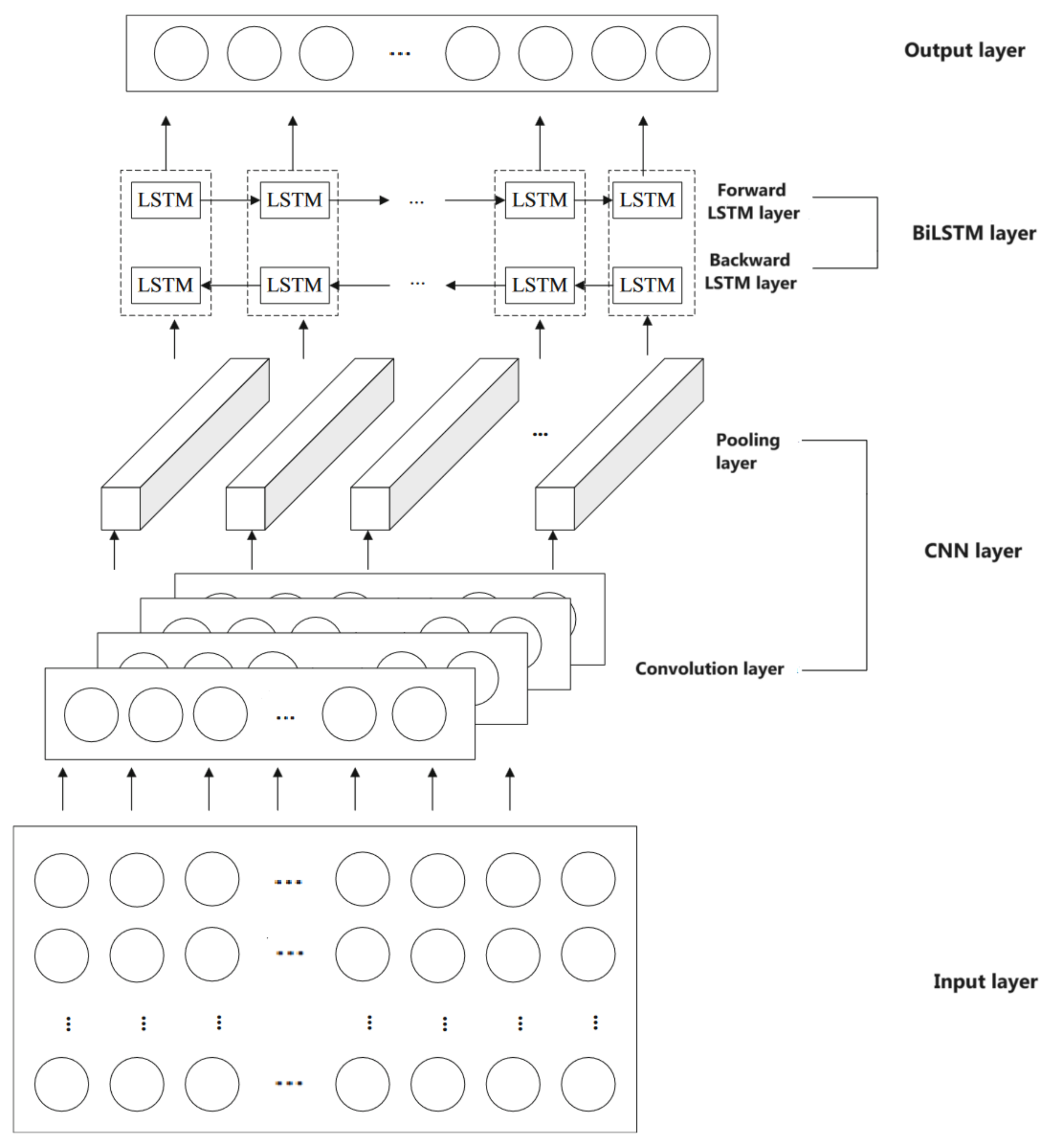Figure 1 shows the model structure diagram. The main structures are CNN and BiLSTM, including the input layer, CNN layer (one-dimensional convolution layer and pooling layer), BiLSTM layer (forward LSTM layer and backward LSTM layer), and output layer.

4.1. CNN

CNN is a network model proposed by (LeCun et al. 1998). It is a feed-forward neural network that performs well in image and natural language processing (NLP). It can be effectively applied to time series prediction (Qin et al. 2018). The local perception and weight sharing of CNN can greatly reduce the number of parameters, thus improving the efficiency of learning models. CNN mainly comprises the convolution, pooling, and full connection layers (Hao and Gao 2020). Each convolution layer contains a plurality of convolution kernels, and its calculation is shown in Equation (10). After the convolution operation of the convolution layer, the data features are extracted. However, the extracted feature dimensions are very high. So, to solve this problem and reduce the cost of training the network, a pooling layer is added after the convolution layer to reduce the feature dimensions (Kamalov 2020):

$${\mathrm{l}}_{\mathrm{t}}=tanh({\mathbf{x}}_{\mathbf{t}}\times {\mathrm{k}}_{\mathrm{t}}+{\mathrm{b}}_{\mathrm{t}})$$

(10)

where ${\mathrm{l}}_{\mathrm{t}}$ is the output value after convolution, $tanh$ is the activation function, ${\mathbf{x}}_{\mathbf{t}}$ is the input vector, ${\mathrm{k}}_{\mathrm{t}}$ is the weight of the convolution kernel, and ${\mathrm{b}}_{\mathrm{t}}$ is the bias of the convolution kernel.

4.2. LSTM

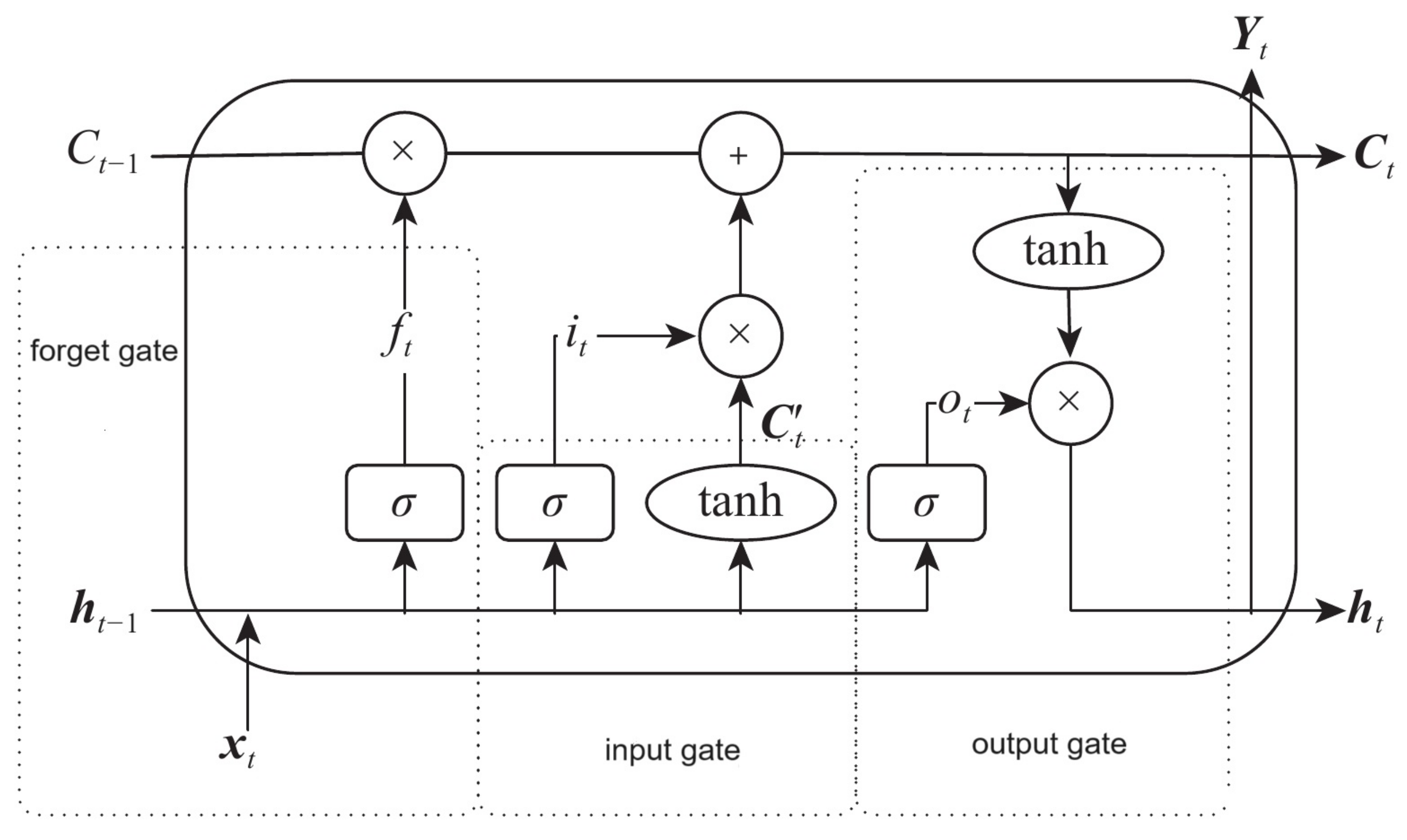
Long Short-Term Memory (LSTM) (Hochreiter and Schmidhuber 1997) is a type of recurrent neural network (RNN) aimed at dealing with the long-standing problems of gradient explosion and gradient disappearance in traditional RNNs (Ta et al. 2020). Its advantage over other RNNs, hidden Markov models, and other sequence learning methods is its relative insensitivity to gap length. It aims to provide a short-term memory for RNN that can last thousands of time steps. The LSTM memory cell consists of three parts—the forget gate, the input gate, and the output gate—as shown in Figure 2. The model utilizes a gate control mechanism to adjust information flow and systematically determines the amount of incoming information retained in each time step.

In Figure 2, $C_{t-1}$ is the cell state of the previous moment, $h_{t-1}$ is the final output value of the LSTM neuronal unit at the last moment, ${\mathbf{x}}_{\mathbf{t}}$ is the input for the current moment, $\sigma$ is the activation function, $f_t$ is the output of the forget gate at the current moment, $i_t$ is the input gate output for the current moment, $C_t^{\prime }$ is the candidate cell status at the current moment, $o_t$ is the output value of the output gate, $C_t$ is the cell state at the current moment, and $h_t$ is the output of the current moment. The working of LSTM is as follows.

Forget Gate

The information that is no longer useful in the cell state is removed with the forget gate. Two inputs, ${\mathbf{x}}_{\mathbf{t}}$ (input at the particular time) and ${\mathrm{h}}_{\mathrm{t}-1}$ (previous cell output), are fed to the gate and multiplied with weight matrices followed by the addition of bias. The result is passed through an activation function, which gives a binary output. If, for a particular cell state, the output is 0, the piece of information is forgotten, and for output 1, the information is retained for future use. The equation for the forget gate is as shown in Equation (11):

$${\mathrm{f}}_{\mathrm{t}}=\sigma ({\mathrm{W}}_{\mathrm{f}}[{\mathrm{h}}_{\mathrm{t}-1},{\mathbf{x}}_{\mathbf{t}}]+{\mathbf{b}}_{\mathbf{f}})$$

(11)

where the value range of ${\mathrm{f}}_{\mathrm{t}}$ is from 0 to 1, ${\mathrm{W}}_{\mathrm{f}}$ represents the weight matrix associated with the forget gate, ${\mathbf{b}}_{\mathbf{f}}$ is the bias of the forget gate, and $[{\mathrm{h}}_{\mathrm{t}-1},{\mathbf{x}}_{\mathbf{t}}]$ denotes the concatenation of the current input and the previous hidden state.

Input gate

The input gate adds useful information to the cell state. First, the information is regulated using the sigmoid function and filters the values to be remembered, similar to the forget gate using inputs ${\mathrm{h}}_{\mathrm{t}-1}$ and ${\mathbf{x}}_{\mathbf{t}}$. Then, a vector is created using the $tanh$ function that gives an output from −1 to +1, which contains all the possible values from ${\mathrm{h}}_{\mathrm{t}-1}$ and ${\mathbf{x}}_{\mathbf{t}}$. Finally, the vector and the regulated values are multiplied to obtain useful information. The equation for the input gate is as shown in Equation (12):

$$\begin{array}{cc}\hfill {\mathrm{i}}_{\mathrm{t}}& =\sigma ({\mathrm{W}}_{\mathrm{i}}[{\mathrm{h}}_{\mathrm{t}-1},{\mathbf{x}}_{\mathbf{t}}]+{\mathbf{b}}_{\mathbf{i}})\hfill \\ \hfill {\mathrm{C}}_{\mathrm{t}}^{\prime }& =tanh({\mathrm{W}}_{\mathrm{c}}[{\mathrm{h}}_{\mathrm{t}-1},{\mathbf{x}}_{\mathbf{t}}]+{\mathbf{b}}_{\mathbf{c}})\hfill \end{array}$$

(12)

where the value range of ${\mathrm{i}}_{\mathrm{t}}$ is from 0 to 1, ${\mathrm{W}}_{\mathrm{i}}$ is the weight of the input gate, ${\mathbf{b}}_{\mathbf{i}}$ is the bias of the input gate, ${\mathrm{W}}_{\mathrm{c}}$ is the weight of the candidate input gate, and ${\mathbf{b}}_{\mathbf{c}}$ is the bias of the candidate input gate.

Multiply the previous state by ${\mathrm{f}}_{\mathrm{t}}$, disregarding the information previously chosen to ignore. Next, include ${\mathrm{i}}_{\mathrm{t}}\odot {\mathrm{C}}_{\mathrm{t}}^{\prime }$. This represents the updated candidate values, adjusted for the amount chosen to update each state value as shown in Equation (13):

$${\mathrm{C}}_{\mathrm{t}}={\mathrm{f}}_{\mathrm{t}}\odot {\mathrm{C}}_{\mathrm{t}-1}+{\mathrm{i}}_{\mathrm{t}}\odot {\mathrm{C}}_{\mathrm{t}}^{\prime }$$

(13)

where the value range of ${\mathrm{C}}_{\mathrm{t}}$ is from 0 to 1, and ⊙ is the Hadamard (element-wise) product operator.

Output gate

The task of extracting useful information from the current cell state to be presented as output is performed by the output gate. First, a vector is generated by applying the $tanh$ function on the cell. Then, the information is regulated using the sigmoid function and filtered by the values to be remembered using inputs ${\mathrm{h}}_{\mathrm{t}-1}$ and ${\mathbf{x}}_{\mathbf{t}}$. Finally, the vector and the regulated values are multiplied to be sent as an output and input to the next cell. The equation for the output gate is shown in Equation (14):

$$\begin{array}{cc}\hfill {\mathrm{o}}_{\mathrm{t}}& =\sigma ({\mathrm{W}}_{\mathrm{o}}[{\mathrm{h}}_{\mathrm{t}-1},{\mathbf{x}}_{\mathbf{t}}]+{\mathbf{b}}_{\mathbf{o}})\hfill \\ \hfill {\mathrm{h}}_{\mathrm{t}}& ={\mathrm{o}}_{\mathrm{t}}\odot tanh\left({\mathrm{C}}_{\mathrm{t}}\right)\hfill \end{array}$$

(14)

where the value range of ${\mathrm{o}}_{\mathrm{t}}$ is from 0 to 1, ${\mathrm{W}}_{\mathrm{o}}$ is the weight of the output gate, and ${\mathbf{b}}_{\mathbf{o}}$ is the bias of the output gate.

4.3. Bidirectional LSTM

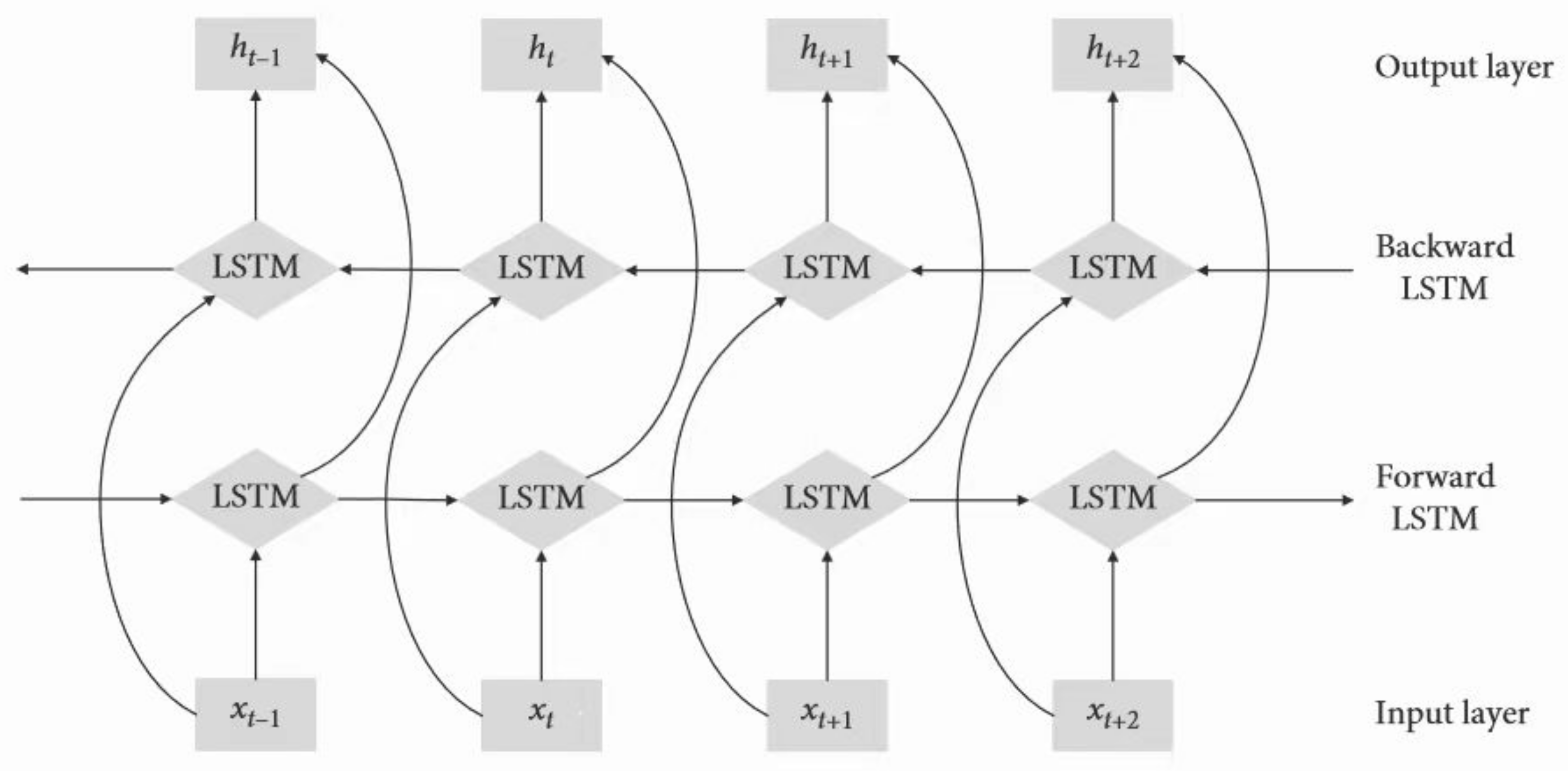
The bidirectional LSTM (BiLSTM) network, which acts as forward and backward LSTM networks for each training sequence, is employed to build a more accurate prediction model. The two LSTM networks are connected to the same output layer to provide complete context information to each sequence point. Figure 3 shows the structure of BiLSTM.

5. Preprocessing for Data from Three Stock Markets

Data used in the simulation were selected from three stock markets: the Shanghai, Hong Kong, and NASDAQ Stock Exchanges. The effectiveness of the prediction model may be affected by the state of the market (Mehtab and Sen 2022). To address this, incorporating data from various market conditions could resolve this issue. The data used in this thesis were taken from the Tushare data platform (https://tushare.pro, accessed on 29 February 2024). Tushare provides a free data interface, including stock, financial statement data, indexes, funds, futures, macroeconomic data, etc.

We obtained the daily historical data of individual stocks in three stock markets from the platform from 2014 to 2021. This includes the historical data of 1655 stocks (main board) in the Shanghai market, 2071 in the Hong Kong market, and 2131 in the NASDAQ market. We also selected the historical data of the Shanghai Stock Exchange Composite Index (SSE Composite Index), Hang Seng Index (HSI), and NASDAQ Composite Index (IXIC).

5.1. Data Preprocessing

Financial data hvae been proven to be noisy and contain a lot of outliers and missing values, which can negatively affect the performance of machine learning models. However, machine learning algorithms require high-quality, relevant, well-structured data to produce accurate predictions. That means the data-processing section is an essential step for this research (Haq et al. 2021). To complete data processing, we removed the missing value, and then the z-score was implemented to detect the outliers and standardization.

The z-score is a statistical method used to determine how many standard deviations a particular data point is from the mean of a dataset. To calculate the z-score, subtract the mean of the dataset from the data point and then divide by the standard deviation of the dataset. A high z-score indicates that the data point deviates significantly from the mean of the dataset and is likely an anomaly. The z-score method is commonly used for data normalization, which involves transforming the data to have a mean of zero and a standard deviation of one. Normalizing the data makes it easier to compare data points measured on different scales and identify patterns and relationships between variables.

5.2. Feature Selection

Feature engineering is creating new features from raw data to improve the model’s predictive performance. This process includes feature extraction, feature selection, and data denoising. We selected three different sets of features, which are OHLC indicators, financial indicators, and technical indicators (Zhang et al. 2014). OHLC indicators are the daily open price, high price, low price, and close price.

Technical indicators are based on historical price and volume data, and are used to analyze patterns and trends in the market. We used the TA-Lib tool (https://ta-lib.github.io/ta-lib-python/index.html, accessed on 26 May 2024) to extract technical indicators related to short-term investment, including overlap studies, momentum, volume, cycle, and volatility indicators (Vargas et al. 2018). For indicators with time parameters, we set the “timeperiod” to 5 days and 10 days, respectively. In this way, we extracted more than 40 technical indicators. It has been proved that these features effectively identify patterns and relationships that may influence future stock prices (Zhai et al. 2007). Part of the technical indicators that have been put into use are shown in

Table 3. Description of technical indicators.

Name	Definition
CMO	The Chande Momentum Oscillator (CMO) is an indicator that calculates the difference between the sum of recent gains and the sum of recent losses and then divides the result by the sum of all price movements over the same period. CMO = 100 × ((Su − Sd) ÷ (Su + Sd)). where Su = Sum of the difference between the current close and previous close on up days for the specified period. Up days are days when the current close is greater than the previous close. Sd = Sum of the absolute value of the difference between the current close and the previous close on down days for the specified period. Down days are days when the current close is less than the previous close.
CCI	The Commodity Channel Index (CCI) is an indicator that measures the difference between the current price and the historical average price. CCI = (Typical Price − SMATP) ÷ (0.015 × Mean Deviation). where SMATP = Simple MA(20) applied to the Typical Price.
SAR	Known as the ‘stop and reversal system’, SAR is an indicator that detects the price direction of an asset and decides how to distribute the attention to the signal of price direction changes.
KAMA	Kaufman’s Adaptive Moving Average (KAMA) is a moving average designed to account for market noise or volatility.
ADX	Average directional index(ADX), an indicator representing the strength of a price trend.
MOM	Momentum can be regarded as the ratio of stock price changes over a period of time. MOM = Price − Price of n periods ago
ROC	Known as the price rate of change, measure the scale of change in price between the current price and the price of a certain historical price. $\mathrm{ROC}=((\mathrm{Closing}{\mathrm{Price}}_p-\mathrm{Closing}{\mathrm{Price}}_{p-n})÷\mathrm{Closing}{\mathrm{Price}}_{p-n})\times 100.$ where $\mathrm{Closing}{\mathrm{Price}}_p$ = Closing price of most recent period. $\mathrm{Closing}{\mathrm{Price}}_{p-n}$ = Closing price n periods before most recent period.

. We also selected market indices and financial indicators. The financial indicators include the p/e ratio, p/b ratio, and price–sales ratio.

Four filtering methods were used to remove irrelevant features:

(1)

Filter the features with missing values (Acuña and Rodriguez 2004);

(2)

Filter the features with unique value (Biswas 2004);

(3)

Filter the features with high correlation with other features (Tang et al. 2014);

(4)

Filter the features with low importance (Kursa et al. 2010).

We computed the Pearson correlation coefficient while filtering the highly correlated features to determine the interrelationships between the features (Liu et al. 2020). It was observed that highly correlated features were associated with computational inefficiencies and a propensity for overfitting. Consequently, variables displaying a correlation of $90\%$ were eliminated from the dataset. Finally, features demonstrating minor importance were eliminated, as they were deemed to have no discernible impact on the model. After data processing and feature selection, we generated 39 features as input variables.

5.3. Data Labeling

In stock market prediction, a common approach for classification involves assigning labels to examples based on the changes in the closing price of stocks. Specifically, two classes are typically employed: “up” and “down”. An example is classified as “up” if the closing price of a stock rises the following day, while it is labeled as “down” if the price decreases. However, this conventional labeling method overlooks the impact of transaction charges associated with market activities. Consequently, examples that incur losses may be mistakenly labeled as profitable if the investment gains fail to cover the transaction costs, such as stamp duty.

This research introduces the labeling scheme incorporating a threshold value denoted as $T_R$ to address this limitation. This threshold is determined based on the stock’s return rate (R). Specifically, if the return rate R exceeds the predefined threshold $T_R$, the corresponding example is categorized as belonging to the profit class. Conversely, the example is classified as a loss if R is less than or equal to $T_R$. Notably, throughout the experiment analysis, a uniform value of $T_R=0.3\%$ is employed as the threshold:

$$Label=\left\{\begin{array}{cc}1\hfill & \mathrm{if}R>T_R\hfill \\ 0\hfill & \mathrm{if}R<=T_R\hfill \end{array}\right.$$

The return rate of the stock is calculated according to the following formula:

$$R=\frac{next\_price}{close\_price}-1$$

where $close\_price$ is the stock closing price, and $next\_price$ is the stock closing price the next day.

By adopting the return label strategy, we can ensure that the labeling strategy does not influence the potential loss incurred through stock trading. This separation of losses from labeling decisions maintains the integrity of the evaluation process.

5.4. Dataset Splitting

In data analysis contests, reserving a test set and making it unknown to all participants is common practice. On the other hand, to increase the generalization ability, the participants often divide the training data into several parts, obtain a model for each part, and use the averaged output of all models to make decisions for the test set. Specifically,

Table 4. Dataset splitting.

	Training Dataset	Testing Dataset
Fold-1	from 1 January 2014 to 31 December 2018	from 1 January 2021 to 31 December 2021
Fold-2	from 1 January 2015 to 31 December 2019	from 1 January 2021 to 31 December 2021
Fold-3	from 1 January 2016 to 31 December 2020	from 1 January 2021 to 31 December 2021

presents the dataset splitting for the stock market prediction analysis. The table outlines data division into training and testing datasets. The training dataset contains three folds from 1 January 2014 to 31 December 2020, representing seven years of historical data. Each fold contains 5 years of historical data. These datasets are utilized to train the model. The corresponding testing dataset covers 2021, from 1 January to 31 December. It is an independent dataset to evaluate the model’s performance and assess its ability to make correct investment decisions for that particular year. The final predicted probability is calculated as the average of the model predictions from training on three data folds.

6. Experiment Setting

This section details the PyTorch platform, hyperparameter optimization, model implementation, backtesting, and performance measurement. All the experiments were conducted under the running environment of an Intel i9-9900K 5.0 GHz, 64 GB of RAM, a graphics card RTX-4090, and Windows 11 Pro.

6.1. PyTorch Platform

PyTorch is an open-source machine learning library developed by Facebook’s AI Research Lab (FAIR) (Paszke et al. 2019). It provides a flexible, user-friendly platform for building and training deep neural networks. PyTorch was designed to be fast, reliable, and scalable, with features such as dynamic computational graphs, memory management automation, and support for CPU and GPU. It is widely used in research and industry for tasks such as image and text classification, object detection, and generative modeling.

6.2. Hyperparameter Optimization

To improve the model further, we utilized the Optuna (Akiba et al. 2019) framework for hyperparameter optimization. Optuna is a tool that automatically searches for the best hyperparameters for a given machine learning model. It employs Bayesian optimization, which selects hyperparameters based on their expected improvement in the objective function.

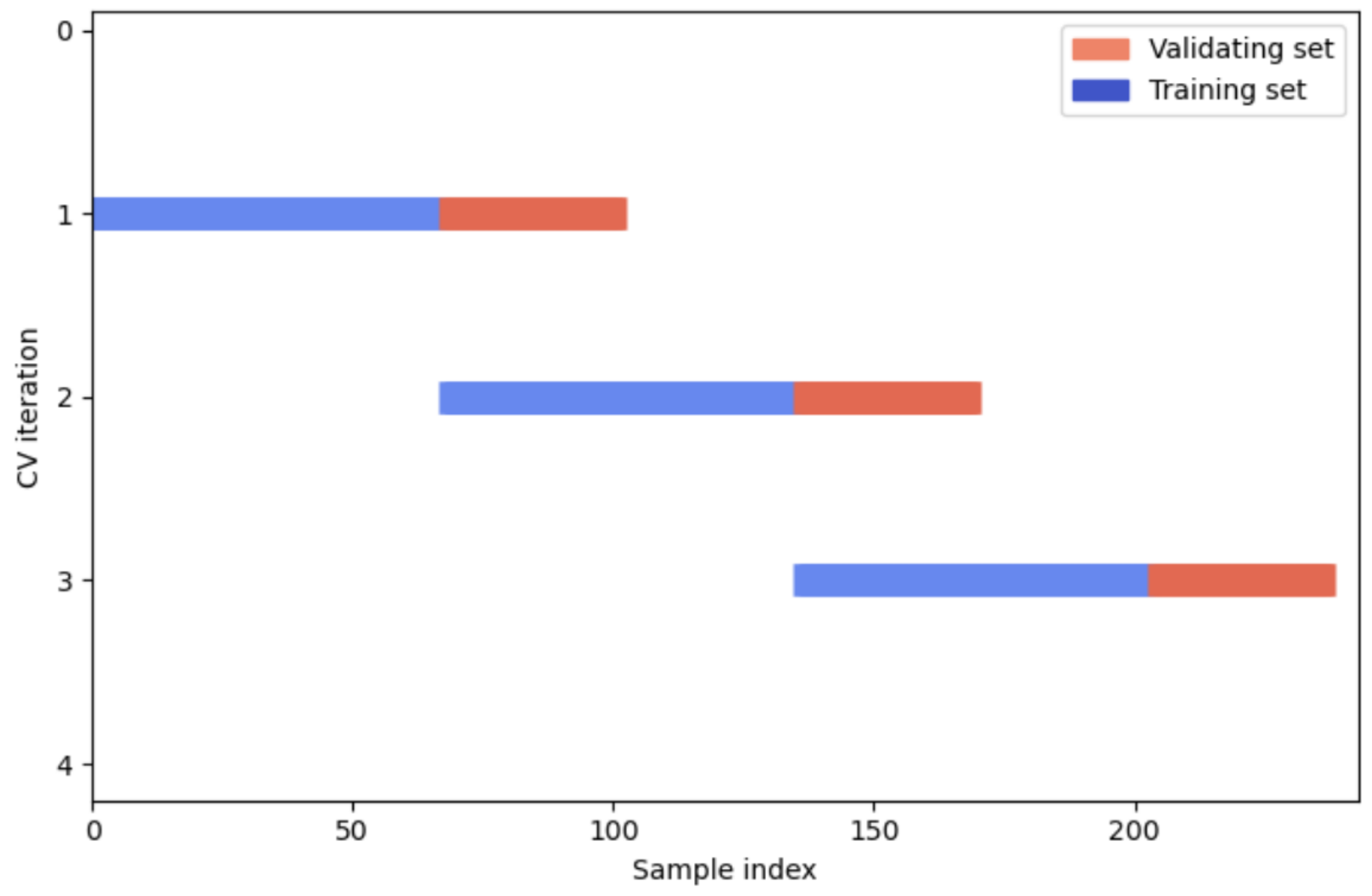
We optimize model hyperparameters using blocking time series cross-validation (Zhao and Liu 2022). In this process, we chronologically divide the entire training dataset into three blocks. Each block comprises a training set and a validating set. Starting from the second block, the training set’s start date aligns with the validation set’s start date from the preceding block as illustrated in Figure 4.

The hyperparameters include ‘batch_size’, ‘hidden_size’, ‘num_layer’, and ‘dropout’ of LSTM, ‘$\beta$’, and ‘$\gamma$’ of GLoss.

6.3. Model Implementation

To prove GLoss CNN-BiLSTM (GL-CNN-BiLSTM)’s effectiveness, it is compared with binary cross entropy LSTM (BCE-LSTM), GL-LSTM, BCE-CNN-LSTM, GL-CNN-LSTM, BCE-BiLSTM, GL-BiLSTM, BCE-CNN-BiLSTM, and GL-CNN-BiLSTM using the same training set and testing set data under the same operating environment. All methods are implemented in Python and Pytorch. GLoss and BCE are used as the evaluation criteria for the methods to evaluate the prediction effect of GL-CNN-BiLSTM.

In addition, since the cost-harmonization loss (CHL) is a special case of GLoss, we simultaneously designed CHL-CNN-LSTM and CHL-CNN-BiLSTM models.

Table 5. Parameter settings of GL-CNN-BiLSTM.

Layer/Loss Function	Parameters	Value
Conv1d 1	in_channels	39
	out_channels	64
	kernel_size	3
	stride	1
	padding	1
	bias	True
	activation function	Sigmoid
MaxPool1d 2	kernel_size	3
	stride	1
	padding	1
LSTM	input_size	64
	hidden_size	64
	num_layer	3
	bias	True
	batch_first	True
	dropout	0.3
	bidirectional	True
FC	in_features	128
	out_features	1
	bias	True
Generalized Loss	$\alpha$	$n_1/n_0$ 3
	$\beta$	2
	$\gamma$	2

¹ Conv1d is a one-dimensional (1D) Convolutional Neural Network (CNN). ² MaxPool1d is a 1D CNN layer that performs a max-pooling operation on the input data. ³ n₁ is the number of positive class and n₀ is the number of negative class.

shows the parameter settings of the GL-CNN-BiLSTM model for the experiment. In the experiment, all the method training parameters are the same: the epoch is 10, the loss functions are BCE, GLoss, and CHL, the optimizer chooses Adamax, the batch size is 256, the time step is 10, and the learning rate is 0.001.

6.4. Backtesting

Backtesting involves building models that simulate trading strategies using historical data aimed to evaluate the performance of the model (Olorunnimbe and Viktor 2023). In this research, the backtesting is based on the prediction results from the classifier; the stocks predicted to be profitable for the next day can participate in simulated trading. The specific steps of the backtesting are as follows.

We first determine the total investment amount and the investment ratio of one stock. Secondly, stocks classified as profitable are sorted in descending order of their predicted probabilities. Finally, the selected stocks are simulated until the total investment is reduced to the limit or all the selected stocks are traded.

Backtesting follows a defined investment strategy. This research focuses on investing over a short period, aiming to generate investment income while maintaining asset liquidity. Drawing on the short-term investment methodology used in the work of Xiaosong and Qiangfu (2021), our longest holding period is five trading days. Therefore, all inventory will be sold within this time frame.

6.5. Performance Measurement

We discuss the measurement of the model in three different aspects: predictive accuracy, profitability, and risk control ability.

(1) AUC

AUC (Area Under Curve) is the area under the receiver operating characteristic curve and is an important measure of classifier performance. Its calculation formula is as follows:

$$AUC={\int }_0^{1}ROC\times \mathrm{d}FPR$$

where $FPR$ is the false positive rate.

(2) Accuracy

Accuracy measures the proportion of correctly classified examples by the classifier, and its calculation formula is as follows:

$$Accuracy=\frac{TP+TN}{TP+FP+TN+FN}$$

where $TP$ is true positive, $TN$ is true negative, $FP$ is false positive, and $FN$ is false negative.

(3) Precision

Precision measures the ability of the classifier to predict positive examples correctly, and its calculation formula is as follows:

$$Precision=\frac{TP}{TP+FP}$$

(4) F score

The F score is a weighted average of precision and recall, with a weight biased towards recall, making it suitable for imbalanced datasets. Its calculation formula is as follows:

$${\mathrm{F}}_{\mathrm{score}}=\left(1+{\rho }^2\right)\times \frac{\mathrm{Precision}\times \mathrm{Recall}}{{\rho }^2\times \mathrm{Precision}+\mathrm{Recall}}$$

where $Recall=TP/(TP+FN)$, $\rho$ is typically set to 2 to emphasize the importance of recall.

(5) Rate Of Return

The rate of return (ROR) measures the percentage change in the value of an investment over a specific period. It can be calculated using the following formula:

$$ROR=\frac{V_f-V_i}{V_i}\times 100\%$$

where $V_i$ is the initial value of the investment, and $V_f$ is the final value of the investment.

(6) Winning Rate

The winning rate (WR) measures the percentage of successful trades from all trades made by the model. It can be calculated using the following formula:

$$WR=\frac{N_{st}}{N_{tt}}\times 100\%$$

where $N_{st}$ is the number of successful trades, and $N_{tt}$ is the total number of trades.

(7) Sharpe Ratio

The Sharpe ratio (SR) measures an investment’s excess return per unit of risk. It can be calculated using the following formula:

$$SR=\frac{R_p-R_f}{{\sigma }_p}$$

where $R_p$ is the portfolio’s expected return, $R_f$ is the risk-free rate, and ${\sigma }_p$ is the portfolio’s standard deviation.

(8) Annual Volatility

The annual volatility (AV) measures the variability of a portfolio’s returns over a year. It can be calculated using the following formula:

$$AV={\sigma }_p\times \sqrt{N}$$

where ${\sigma }_p$ is the portfolio’s standard deviation, and N is the number of trading days in a year.

7. Experimental Results

The Shanghai, Hong Kong, and NASDAQ stock market datasets from 2014 to 2020 are chosen for three-fold cross-training. The final predicted probability for 2021 equals the average of the corresponding model predictions after training on three data folds. The proposed model’s performance is evaluated based on predictive accuracy, profitability, and risk control capabilities.

Table 6. Performance of models obtained using various methods for the Shanghai Stock Market.

	Metrics	AUC	Accuracy	Precision	F2	ROR	WR	SR	AV
Group-1 a	BCE-LSTM	0.5241	0.5437	0.4531	0.5316	0.0443	0.5101	0.14	731.77
	GL-LSTM	0.5149	0.5578	0.4561	0.5203	0.0454	0.5274	0.19	620.59
	BCE-CNN-LSTM	0.5293	0.5637	0.4771	0.5247	0.1432	0.5352	0.85	246.70
	GL-CNN-LSTM	0.5378	0.5653	0.4823	0.5245	0.1814	0.5344	1.02	218.22
	CHL-CNN-LSTM	0.5313	0.5650	0.4793	0.5215	0.1789	0.5360	1.13	199.26
Group-2 b	BCE-BiLSTM	0.5220	0.5649	0.4746	0.5167	0.0121	0.5193	−0.06	1558.08
	Gl-BiLSTM	0.5295	0.5704	0.5410	0.4997	0.0391	0.5945	0.40	303.88
	BCE-CNN-BiLSTM	0.5281	0.5635	0.4796	0.5291	0.1327	0.5200	0.74	275.79
	GL-CNN-BiLSTM	0.5293	0.5560	0.4642	0.5303	0.1664	0.5247	0.85	251.91
	CHL-CNN-BiLSTM	0.5272	0.5591	0.4672	0.5272	0.2153	0.5300	1.21	190.94
Group-3 c	BCE-LightGBM	0.5555	0.5722	0.5097	0.5368	0.1258	0.5161	0.58	330.90
	CHL-LightGBM	0.5553	0.5721	0.5085	0.5399	0.2104	0.5171	0.97	230.81
	FL-LightGBMM	0.5555	0.5726	0.5107	0.5389	0.1620	0.5172	0.75	278.81

^a Methods related to LSTM. ^b Methods related to BiLSTM. ^c Methods related to LightGBM.

,

Table 7. Performance of models obtained using various methods for the Hong Kong Stock Market.

	Metrics	AUC	Accuracy	Precision	F2	ROR	WR	SR	AV
Group-1 a	BCE-LSTM	0.5411	0.5526	0.5003	0.5028	1.1411	0.5559	5.53	52.02
	GL-LSTM	0.5380	0.5536	0.5041	0.5135	2.2306	0.5549	9.32	39.74
	BCE-CNN-LSTM	0.5402	0.5536	0.5037	0.5168	3.3483	0.5534	11.30	39.30
	GL-CNN-LSTM	0.5444	0.5120	0.4689	0.5028	4.6503	0.5610	15.65	33.70
	CHL-CNN-LSTM	0.5422	0.5481	0.4935	0.5428	3.6878	0.5585	12.37	37.68
Group-2 b	BCE-BiLSTM	0.5434	0.5573	0.5206	0.5143	1.9487	0.5552	8.80	39.86
	Gl-BiLSTM	0.5428	0.5595	0.5237	0.5239	2.9197	0.5585	10.96	38.08
	BCE-CNN-BiLSTM	0.5365	0.5534	0.5040	0.5062	3.0140	0.5609	11.72	36.20
	GL-CNN-BiLSTM	0.5380	0.5100	0.4666	0.5024	3.6630	0.5545	13.19	35.33
	CHL-CNN-BiLSTM	0.5369	0.5431	0.4863	0.5380	3.0732	0.5487	10.39	40.97
Group-3 c	BCE-LightGBM	0.5522	0.5623	0.5298	0.5292	3.1909	0.6064	13.56	32.27
	CHL-LightGBM	0.5539	0.5637	0.5277	0.5383	4.1944	0.5791	16.42	30.56
	FL-LightGBMM	0.5562	0.5673	0.5464	0.5340	3.9349	0.6053	17.44	27.92

^a Methods related to LSTM. ^b Methods related to BiLSTM. ^c Methods related to LightGBM.

and

Table 8. Performance of models obtained using various methods for the NASDAQ Stock Market.

	Metrics	AUC	Accuracy	Precision	F2	ROR	WR	SR	AV
Group-1 a	BCE-LSTM	0.5238	0.5551	0.5151	0.4996	0.1585	0.5415	1.00	222.54
	GL-LSTM	0.5186	0.5281	0.4658	0.5242	0.2895	0.4901	0.92	248.84
	BCE-CNN-LSTM	0.5067	0.5051	0.4498	0.5054	0.3420	0.4965	1.14	213.71
	GL-CNN-LSTM	0.5224	0.5541	0.5041	0.5146	0.8697	0.5132	3.25	100.12
	CHL-CNN-LSTM	0.5158	0.5565	0.5140	0.5159	0.4765	0.5147	1.99	138.87
Group-2 b	BCE-BiLSTM	0.5286	0.5525	0.4982	0.5168	0.2405	0.5134	1.09	216.86
	Gl-BiLSTM	0.5275	0.5576	0.5299	0.5045	0.2603	0.5283	1.47	65.78
	BCE-CNN-BiLSTM	0.5205	0.5524	0.4974	0.5107	0.3428	0.5141	1.64	157.78
	GL-CNN-BiLSTM	0.5346	0.5590	0.5209	0.5226	0.6037	0.5058	2.16	134.21
	CHL-CNN-BiLSTM	0.5241	0.5517	0.4954	0.5168	0.3467	0.5073	1.44	177.37
Group-3 c	BCE-LightGBM	0.5192	0.5417	0.4621	0.5196	0.9660	0.5288	4.06	84.35
	CHL-LightGBM	0.5205	0.5393	0.4643	0.5247	1.4733	0.5315	5.26	74.65
	FL-LightGBMM	0.5199	0.5383	0.4564	0.5180	1.0771	0.5325	4.53	78.30

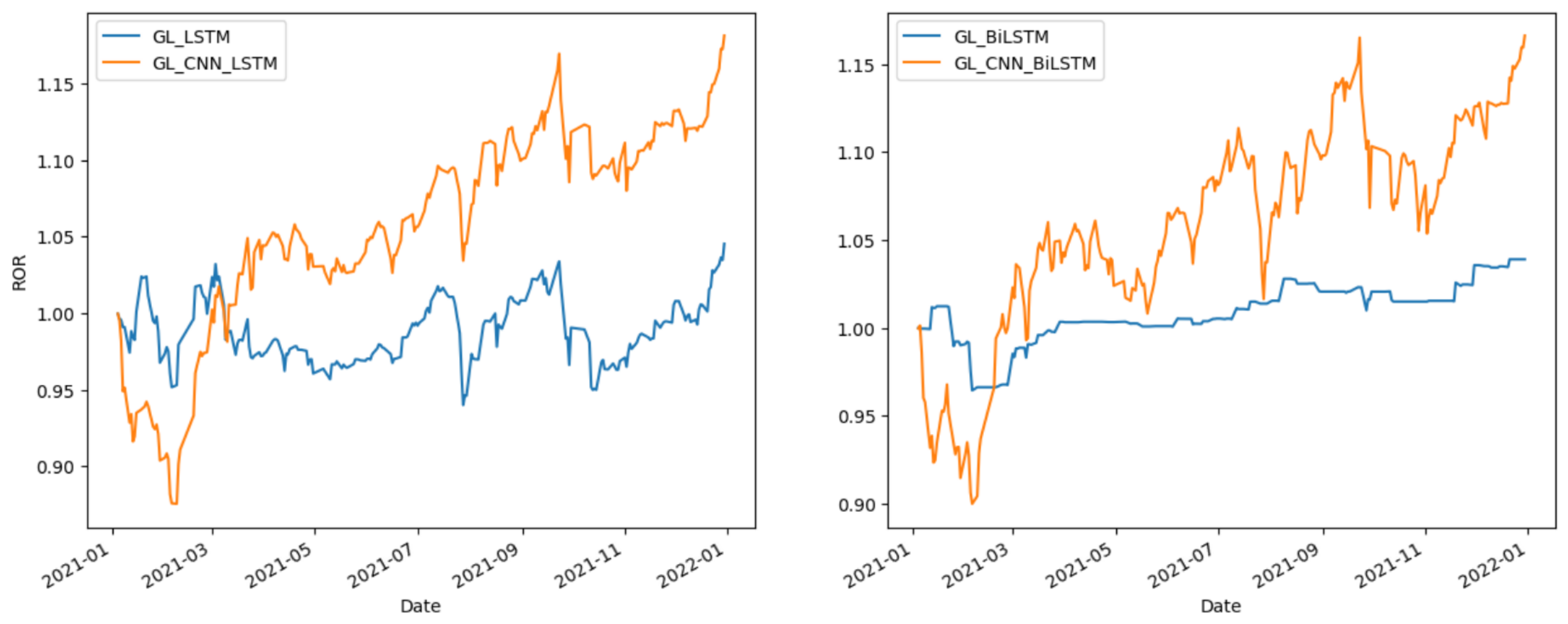
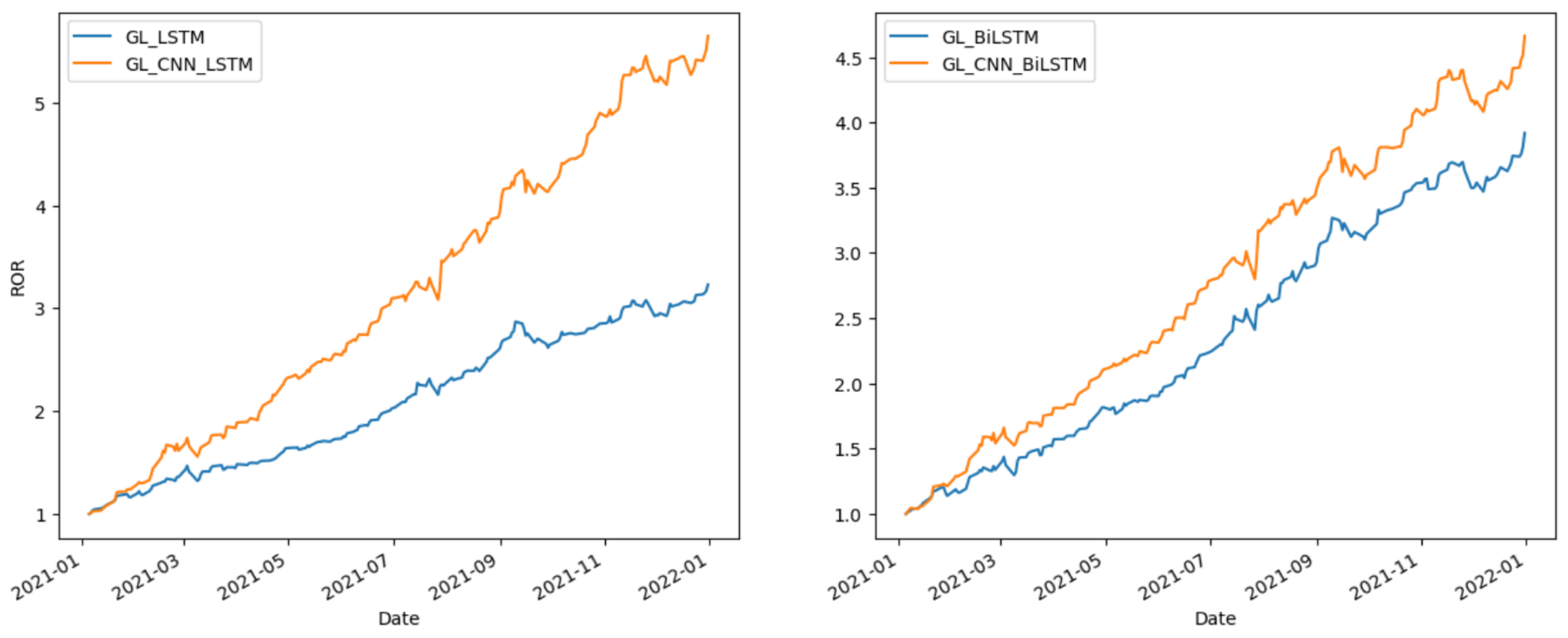
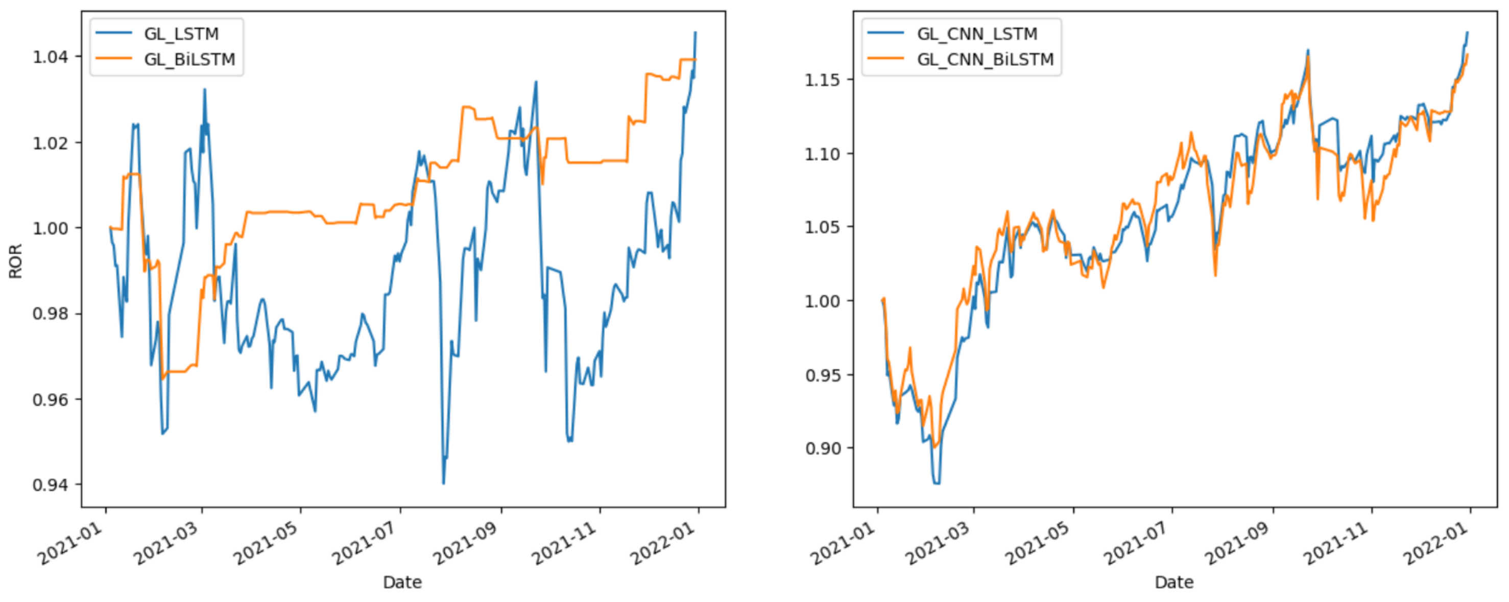
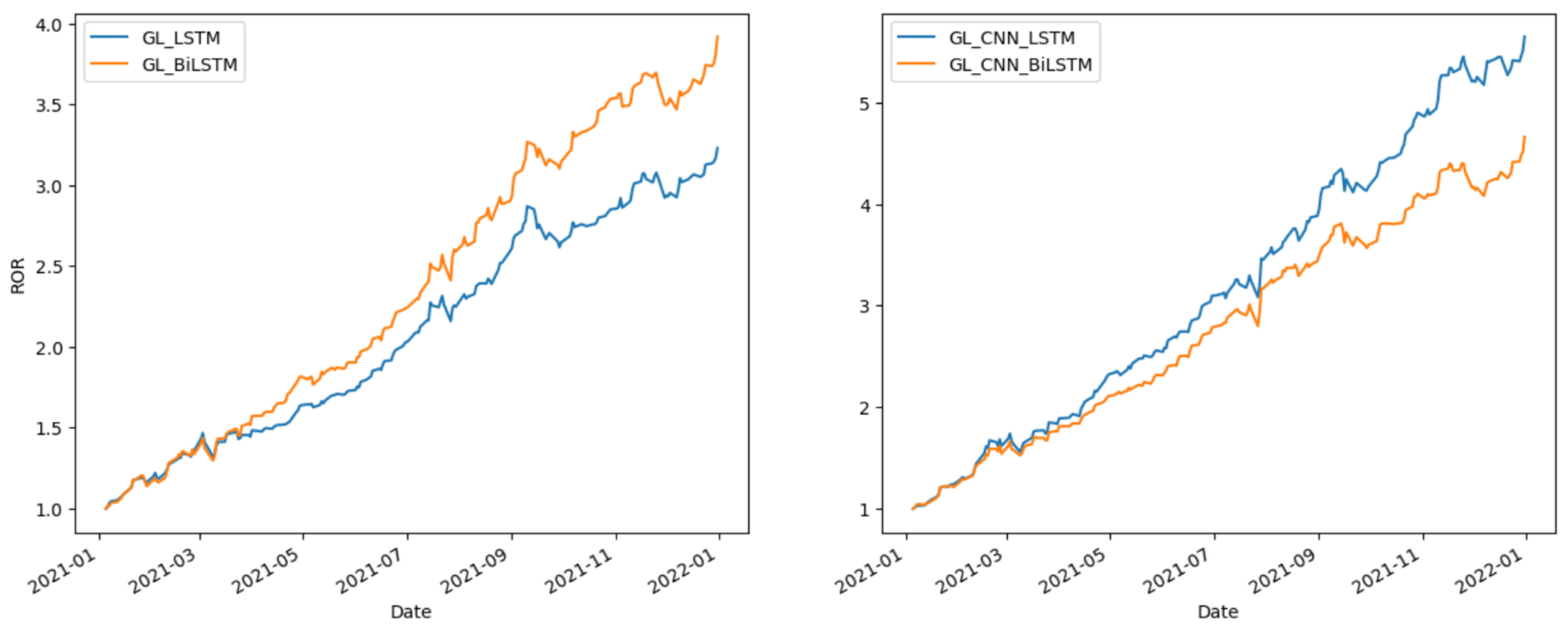
^a Methods related to LSTM. ^b Methods related to BiLSTM. ^c Methods related to LightGBM.

present the performance comparison of different methods, including three groups of methods, on predicting stock market trends. The evaluation metrics used in the analysis are AUC, Accuracy, Precision, F2, ROR, WR, SR, and AV. The test dataset includes data from 2021 for Shanghai, Hong Kong, and NASDAQ stock markets. The results show that the GL-CNN-LSTM and GL-CNN-BiLSTM, including CHL-CNN-LSTM and CHL-CNN-BiLSTM, methods outperformed the other methods in F2, ROR, SR, and AV.

The experimental results of Group-3 are quoted from our early research (Zhao et al. (2023)). By comparison, we can observe that LightGBM may outperform LSTM when dealing with large datasets.

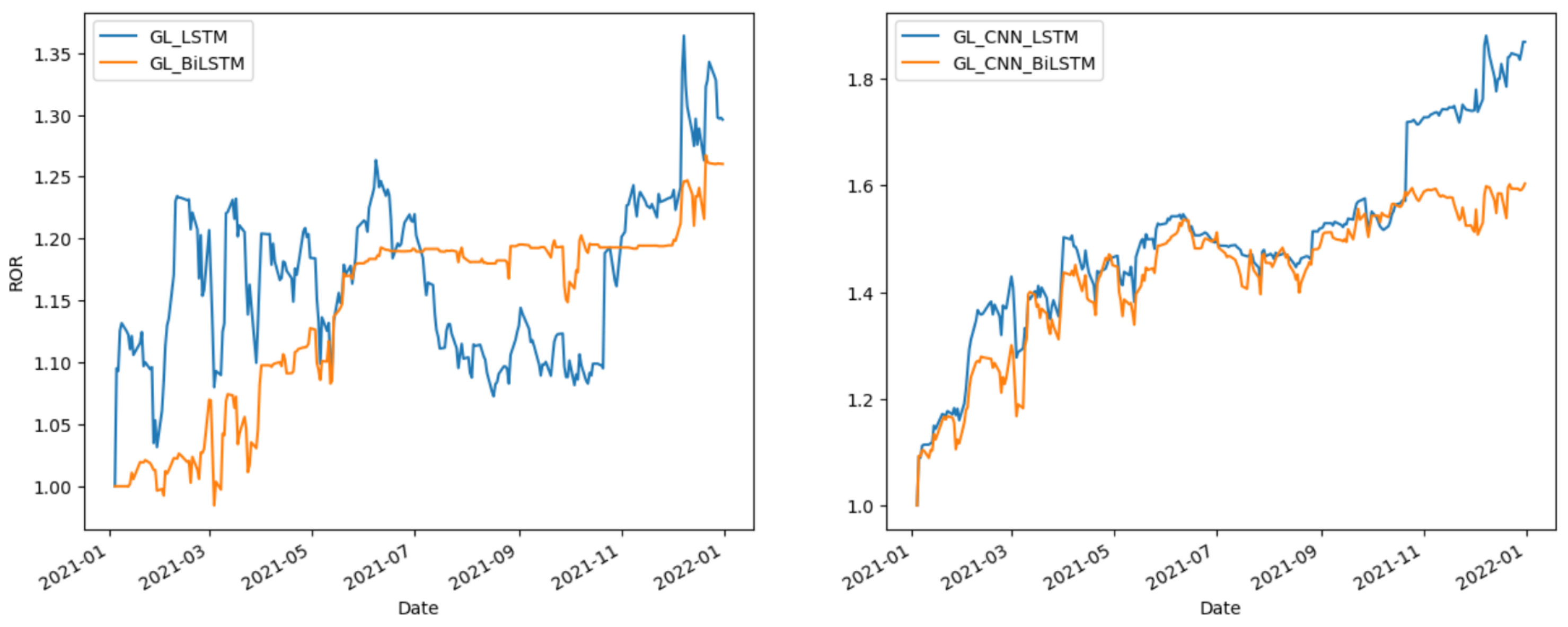
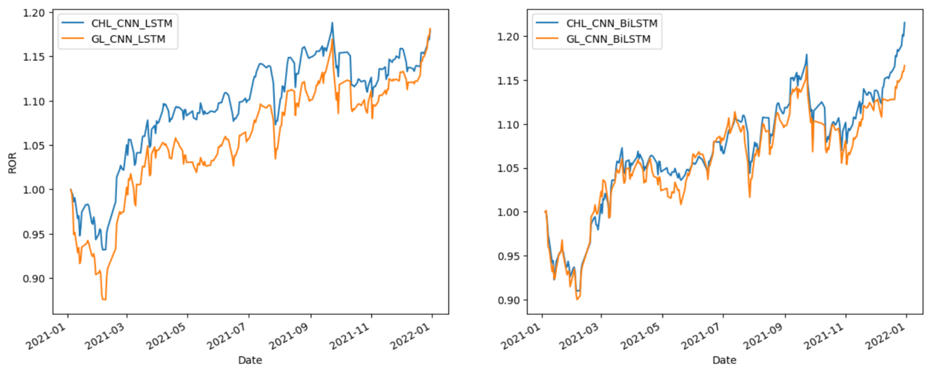
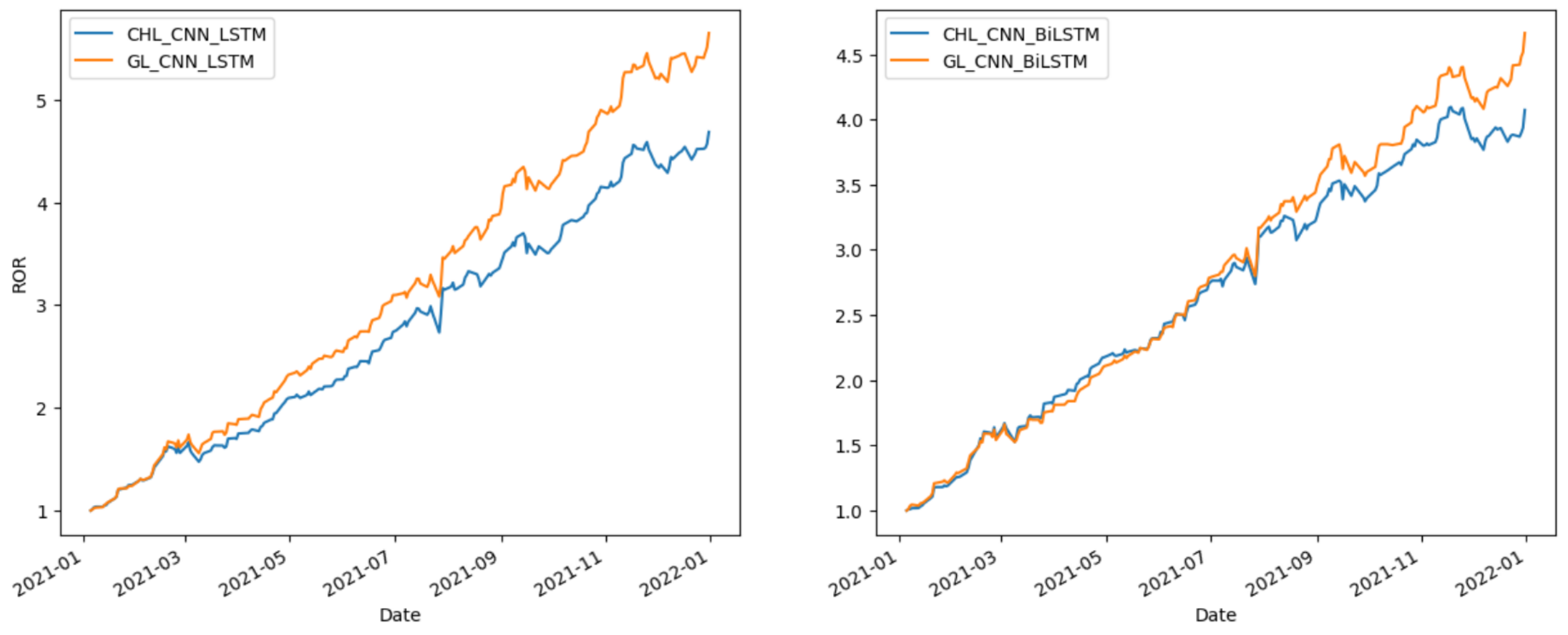
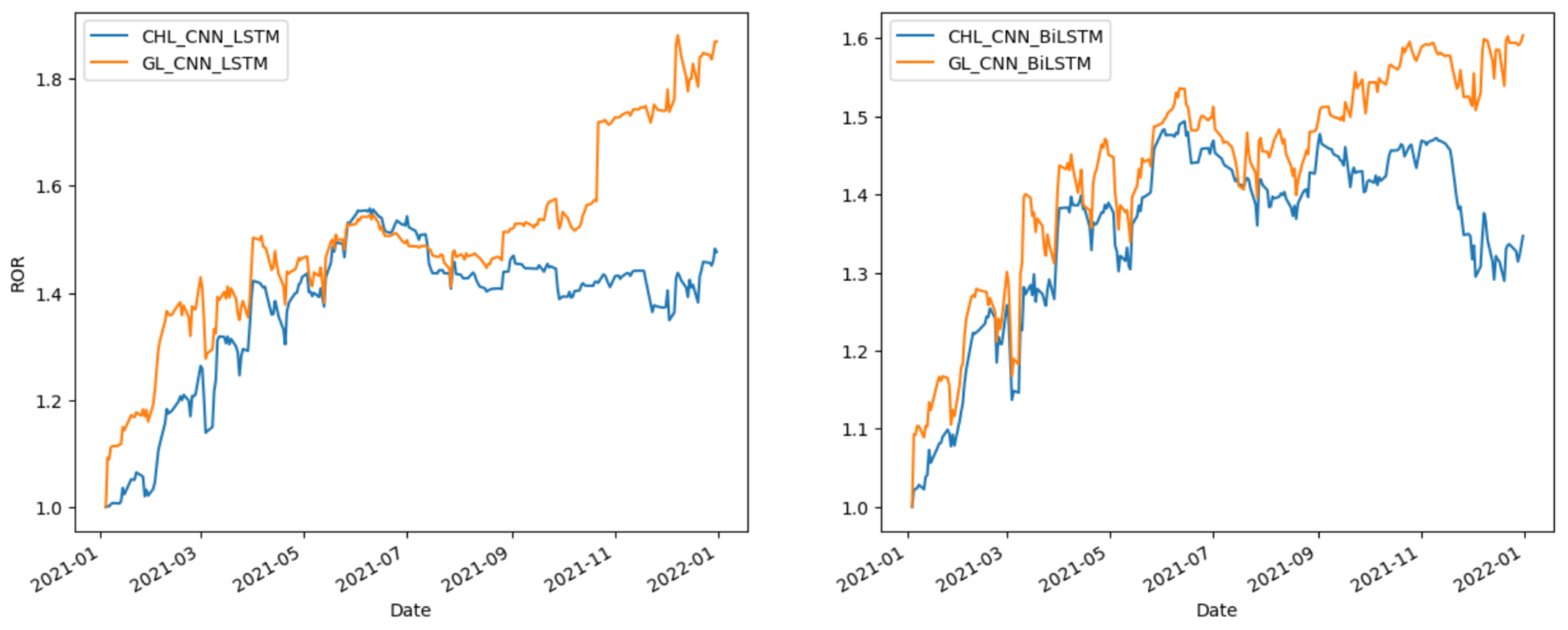
Figure 5, Figure 6 and Figure 7 provide the comparative analysis of the methods related to CNN-LSTM and CNN-BiLSTM in different markets during 2021. This shows that GL-CNN-LSTM and GL-CNN-BiLSTM consistently demonstrate excellent performance in terms of ROR. These observations indicate that utilizing GLoss, CNN-LSTM, or CNN-BiLSTM can significantly enhance stock returns in stock prediction.

Figure 8, Figure 9 and Figure 10 compare the effects of LSTM and BiLSTM. The results indicate that BiLSTM outperforms LSTM in terms of investment return stability.

Figure 11, Figure 12 and Figure 13 compare the effects of CHL and GLoss. As a special case of Gloss, CHL has the same performance as Gloss. On some occasions, CHL performs particularly well, for example, in the Shanghai stock market.

From the predictive accuracy perspective, the evaluation metrics of the proposed models differ by less than $0.03$ from those of other models and show the same results in the three stock markets. However, the ROR of the proposed models differs significantly from that of other models. The Hong Kong stock market outperforms the other two.

The proposed models show better risk control than others, with a higher Sharpe ratio and lower annual volatility. The Hong Kong stock market has the highest Sharpe ratio and the lowest annual volatility among the three stock markets.

Based on the above observations, the proposed model has similar accuracy metrics to others, but the ROR and Sharpe ratios differ significantly. We can explain the reason from the internal principle of the proposed model. GLoss introduces the cost-sensitive mechanism into the CNN-LSTM model. Under the joint effect of the error type factor (cost factor) and the difficulty factor, the model pays more attention to instances with high cost and difficulty during the training process, and the prediction of such instances should be more accurate. Therefore, compared with other models, the prediction results should be a small cost in the False Positive (FP) instances and a large cost in the True Positive (TP) instances. In this way, when conducting transaction backtesting, the proposed models may manage risk better and predict large gains with low frequency; that is, even fewer transactions can bring higher returns and lower annual volatility, resulting in higher Sharpe ratios. Therefore, the level of return and Sharpe ratio have a low correlation with accuracy.

8. Conclusions

The experimental results indicate that the CNN-LSTM model with the generalized loss function performs exceptionally well when applied to the Shanghai, Hong Kong, and NASDAQ Stock Exchange data. Compared to traditional models using the BCE loss function, the model with the generalized loss function demonstrates significant improvements in predictive accuracy and robustness. Moreover, by adjusting different cost factors, the model can better adapt to various market conditions, thereby enhancing the practical applicability of the predictions. These results validate the effectiveness of the generalized loss function in stock prediction, offering valuable insights for future research and applications.

The GL-CNN-BiLSTM and GL-CNN-LSTM models demonstrate favorable investment returns and risk control capabilities as evidenced by their lower annual volatility. They also exhibit good risk-adjusted returns and a high Sharpe ratio.

Our goal in introducing cost-sensitive mechanisms into machine learning is to develop a set of cost-aware algorithms that use machine learning to learn from historical data and continuously improve the cost-minimization strategies, adjust the strategies based on real-time market conditions (such as volatility and liquidity), and slow down or speed up transactions to minimize costs. In future research, we will incorporate practical considerations such as transaction costs and improve cost-aware algorithms. This will help to enhance the performance and feasibility of stock market prediction models, enabling traders and investors to align their strategies with real-world trading environments and improve their risk-adjusted returns.