Probability Distributions for Modeling Stock Market Returns—An Empirical Inquiry

Abstract

Investing in stocks and shares is a common strategy to pursue potential gains while considering future financial needs, such as retirement and children’s education. Effectively managing investment risk requires thoroughly analyzing stock market returns and making informed predictions. Traditional models often utilize normal variance distributions to describe these returns. However, stock market returns often deviate from normality, exhibiting skewness, higher kurtosis, heavier tails, and a more pronounced center. This paper investigates the Laplace distribution and its generalized forms, including asymmetric Laplace, skewed Laplace, and the Kumaraswamy Laplace distribution, for modeling stock market returns. Our analysis involves a comparative study with the widely-used Variance-Gamma distribution, assessing their fit with the weekly returns of the S&P 500 Index and its eleven business sectors, drawing parallel inferences from international stock market indices like IBOVESPA and KOSPI for emerging and developed economies, as well as the 20+ Years Treasury Bond ETFs and individual stocks across varied time horizons. The empirical findings indicate the superior performance of the Kumaraswamy Laplace distribution, which establishes it as a robust alternative for precise return predictions and efficient risk mitigation in investments.

1. Introduction

Forecasting stock market returns relies on advanced financial time series analysis, with probability distributions serving as fundamental components in statistical modeling (Taylor 2008). The fitting of parametric distributions to the statistical characteristics of stock indices returns is integral to econometrics, and holds practical implications for effective risk management. The identification of an accurate distribution for stock indices returns establishes a critical benchmark for evaluating investment success, given that decision-making often hinges on empirical data assessments.

Within the domain of financial economics, a nuanced understanding of stock market return behavior is pivotal. The interplay between stock prices and returns is instrumental in determining potential profits for investors. As a result, the financial literature incorporates sophisticated analytical models that accommodate the non-linear dynamics inherent in stock price fluctuations (Pokharel et al. 2022). Researchers spanning academia and trading circles exhibit a pronounced interest in the statistical modeling of financial asset returns. The initial step in any predictive analysis of significance involves the meticulous determination of the statistical distribution characterizing the phenomenon under scrutiny. While historical suggestions favor normal variance models for stock market return distributions (Praetz 1972), such models often fall short, given the distinctive features of stock returns—displaying a higher peak and heavier tails than what the Gaussian probability distribution predicts.

Some challenges within stock index research revolves around the volatility and it has attracted attention of many scholars who have explored them through the Barndorff-Nielsen and Shephard (BN-S) model. Both the conventional BN-S model and its generalizations have proven instrumental in addressing diverse phenomena such as jumps, stochastic fluctuations, and leverage effects. Interested readers are referred to the pioneering works by Shephard and Barndorff-Nielsen (2001), Kallsen et al. (2011), and SenGupta (2016).

Furthermore, Durham (2007) emphasizes the critical understanding of volatility dynamics and return distribution shapes in finance, proposing the stochastic volatility model (SV-mix model) as a discrete mixture of normals to capture the conditional distribution. This approach provides enhanced insight into return distribution tails and demonstrates empirical superiority over competing models like the single-factor volatility model. In empirical finance, conditional distributions of financial returns are often established through standardized error distributions within GARCH-type models. Chen (2015) introduced the maximum entropy (MaxEnt) approach, presenting a method for moment combination and selection to tackle this distribution-building challenge. This framework proves valuable in unifying and comparing existing distribution specifications, crafting more fitting distribution specifications, and illuminating the significance of various moments in the distribution-building process. This proposition is validated through an empirical investigation on stock index returns. Nevertheless, amidst these efforts, there remains a significant quest for precision for uncovering the exact distribution of returns for stock indices. Finding the exact distribution of returns of stock indices could provide a useful benchmark to measure the success of investment, since stock investment decisions always rely on assessments of the distribution of expected stock returns, which could be obtained from empirical data. Thus, establishing an accurate distribution of stock index returns stands not only as a scholarly pursuit, but also as a practical necessity for investors seeking to make informed decisions.

The Laplace and related distributions are obvious candidates to replace Gaussian models and processes in modeling financial asset returns, because traditional Gaussian distribution models are frequently not supported by real-world data due to fat tails and asymmetry prominent in financial data (Franczak et al. 2013). Laplace distributions are used to fit the marginal distribution function, which will then be employed in a copula function because they can account for leptokurtic and skewed data (Kotz et al. 2001). Compared to the Gaussian distribution, it typically better describes stock return behavior while capturing the greater peak and heavy tails (Nadaf et al. 2022). Recognizing the rarity of stock market data adhering strictly to a standard Laplace distribution, introducing the generalized Laplace distribution enhances flexibility for modeling real-life data.

Empirical research underscores the appropriateness of the skew Laplace distribution in modeling asset returns data, offering a parametric solution to control skewness (Aryal and Nadarajah 2005). The Kumaraswamy Laplace distribution finds application across diverse fields, including medicine, environmental science, economics, engineering, and finance, among others, due to its adaptability (Aryal and Zhang 2016). The asymmetric Laplace distribution exhibits general asymmetry, high peaks, and heavier tails than the normal distribution, is used to model data, and has applications in communication, economics, engineering, and finance (Kotz et al. 2012). The class of asymmetric Laplace distributions is well suited for modeling phenomena where the variable of interest is the result of a significant number of independent, random observations, and the empirical distribution appears to be asymmetric, with a steep peak and heavier tails than those permitted by the normal distribution (Jayakumar and Kuttykrishnan 2007).

The four-parameter Variance-Gamma (V-G) distribution, proposed by Madan and Seneta (1990), occupies a prominent position in finance literature as a potent model for stock returns. The V-G is a continuous statistical distribution, referred to as the generalized Laplace or Bessel function distribution. The V-G distribution’s significant characteristic is that its tails decelerate more slowly than the normal distribution. As a result, it is thought to be exceptionally well-suited for simulating returns on financial assets and turbulent wind speeds.

This article delves into the potential of probability distributions within the Laplace family for modeling stock return predictions, supported by empirical evidence derived from real market data spanning various indices. Acknowledging the absence of a universal probability distribution applicable to all financial data types, our objective is to discern the most suitable distribution for predictive modeling of stock returns. Evaluating the performance of the Variance-Gamma distribution against four-parameter distributions like Kumaraswamy Laplace across eleven S&P 500 business sectors and the index as a whole, our study, based on log-likelihood and AIC criteria, reveals Kumaraswamy Laplace as a superior alternative to Variance-Gamma for modeling stock index returns in eleven out of twelve indices, including the S&P 500 index. The Variance-Gamma distribution marginally performs better than the Kumaraswamy Laplace distribution in fitting the Consumer Discretionary index. Our research suggests that Kumaraswamy Laplace is a potent alternative substitute for Variance-Gamma distribution when modeling stock index returns. This significant finding not only encourages further exploration, but also sparks discussion within the realm of applied finance.

The remaining part of the manuscript is organized as follows. Section 2 describes various generalizations of Laplace distributions, which are used to model the stock return data. Section 3 discusses the data description and methodology used to derive the conclusion. Section 4 discusses the analysis of data. This section is further divided into eleven subsections: each subsection is dedicated to individual business sectors of S&P 500 index and the index itself. Section 5 outlines the ranking of distributions for modeling stock returns, while Section 6 explores exceedance probability and return level prediction. Section 7 includes parallel inferences and some discussions, and Section 8 offers concluding remarks.

2. Generalization of Laplace Distribution

It is of great interest to many investors, portfolio managers, and others to model the returns of their investments, especially stocks. Like any financial modeling problem, fitting a model to stock returns (daily, weekly, or monthly) is difficult, as the returns patterns can drastically change due to many internal and external influences on the stock price or the market more generally. Probability distribution plays a key role in describing and predicting real-world phenomena. Probabilistic modeling and statistical analysis of the behavior of stock market returns are important in finance and economics for assessing risk analysis and providing a means to identify the pattern from the existing data. There are hundreds of discrete and continuous probability distributions in the literature. The data under study may guide us in the choice of distribution among parametric distributions. For example, choice among symmetric versus asymmetric distribution, long-tailed vs. short-tailed distribution, distribution with threshold parameter, among others. Among the prominent probability distributions, the Laplace distribution holds a special place in the modeling financial data.

The Laplace family distribution, with its heavier tails compared to the normal distribution, better captures extreme events such as market crashes or sudden spikes in stock market that influence stock returns. Its robustness to outliers, such as corporate scandals or geopolitical events, enhances modeling reliability. Additionally, its symmetry around the mean accommodates both positive and negative returns without assuming skewness, unlike some traditional distributions. With flexibility in modeling various parameters, it can tailor distributions to fit specific data characteristics. In this article, we will explore the statistical modeling of stock index data using Laplace and some generalized distributions that are derived using the genesis of Laplace distribution.

2.1. Laplace Distribution

The Laplace distribution is named after the French astronomer, mathematician, and physicist Marquis Pierre Simon de Laplace (1749–1827), and is one of the earliest distributions introduced in the probability theory. Laplace distribution is also known as double-exponential distribution, as well as the two-tailed distribution. It is a symmetric distribution whose tails fall off less sharply than the Gaussian distribution and has a cusp, discontinuous first derivative at the mean. The Laplace distribution has been quite commonly used as an alternative to the normal distribution in robustness studies, including the stock returns. An in-depth study of the Laplace distribution, including various properties and applications, is provided in Kotz et al. (2012).

The Laplace distribution has the probability density function (pdf) given by

$$\begin{array}{ccc}\hfill f\left(x\right)& =& {\displaystyle \frac{1}{2\sigma }\exp \left(-\frac{\mid x-\mu \mid }{\sigma }\right),}\hfill \end{array}$$

(1)

where $-\infty <x<\infty$, $\sigma >0$ and $-\infty <\mu <\infty$. The expected value, $E\left(X\right)$, and the variance, $\mathrm{Var}\left(X\right)$, of a Laplace random variable respectively given by

$$\begin{array}{ccc}\hfill E\left(X\right)& =& \mu \hfill \\ \hfill Var\left(X\right)& =& 2{\sigma }^2.\hfill \end{array}$$

It should be noted that the median and the mode of the Laplace distribution are the same as its mean $\mu$. Since the generalized distribution allows more flexibility to model real-world data, there has been a growing interest in developing a generalized class of distribution by inducting one or more additional parameter(s). Several asymmetry forms of Laplace distribution have appeared in the literature, including those introduced by McGill (1962), Holla and Bhattacharya (1968), Lingappaiah (1988), Poiraud-Casanova and Thomas-Agnan (2000), Kozubowski and Podgorski (2000), Gupta et al. (2002), Kozubowski and Nadarajah (2008), and Cordeiro and Lemonte (2011), to name a few. A comprehensive review of variations of the univariate Laplace distribution is provided in Kozubowski and Nadarajah (2010).

2.2. Asymmetric Laplace Distribution

A random variable X is said to have an asymmetric Laplace distribution (ALD) with location parameter $\mu$, scale parameter $\sigma >0$, and skewness parameter $p\in (0,1)$, if its probability density function (pdf) is given by

$$\begin{array}{c}\hfill f(x,\mu ,\sigma ,p)=\frac{p(1-p)}{\sigma }\exp \left\{-{\rho }_p\left(\frac{x-\mu }{\sigma }\right)\right\},\end{array}$$

where ${\rho }_p\left(u\right)=u(p-I_{u<0})$ is the loss function, with $I(.)$ denoting the usual indicator function. The support of the random variable X is the real line and the loss function $\rho$ assigns weight p or $1-p$ to the observations greater or, respectively, less than $\mu$ and that $Pr(X\le \mu )=p$. Therefore, the distribution splits along the scale parameter into two parts, one with probability p to the left, and one with probability $(1-p)$ to the right. Note that the ALD is skewed to the left when $p>\frac{1}{2}$, and skewed to the right when $p<\frac{1}{2}$. It should be noted that for $p=\frac{1}{2}$, the ALD reduces to double exponential distribution with its pdf

$$\begin{array}{c}\hfill f(x,\mu ,\sigma ,\frac{1}{2})=\frac{1}{4\sigma }exp\left(-\frac{\mid x-\mu \mid }{2\sigma }\right).\end{array}$$

(2)

The expected value, $E\left(X\right)$, and the variance, $\mathrm{Var}\left(X\right)$, of X are respectively given by

$$\begin{array}{ccc}\hfill E\left(X\right)& =& \mu +\frac{\sigma (1-2p)}{p(1-p)}\hfill \\ \hfill Var\left(X\right)& =& \frac{{\sigma }^2(1-2p+2p^2)}{{(1-p)}^2{p}^2}.\hfill \end{array}$$

Readers are referred to Yu and Zhang (2005) for details.

2.3. Skew Laplace Distribution

A random variable X is said to have the skew-Laplace distribution if its probability density function is $f\left(x\right)=2g\left(x\right)G\left(\lambda x\right)$, where $g\left(x\right)$ and $G\left(x\right)$ are the pdf and cdf of the Laplace distribution and $\lambda$ is the skewness parameter. One can consider the case of $\lambda >0$, as the corresponding results for $\lambda <0$ can be obtained using the fact that $-X$ has the pdf given by $2g\left(x\right)G(-\lambda X)$. When $\lambda >0$, the pdf of skew Laplace distribution is given by

$$\begin{array}{ccc}\hfill f\left(x\right)& =& {\displaystyle \left\{\begin{array}{cc}{\displaystyle \frac{1}{2\sigma }\exp \left\{\frac{(1+\lambda )(x-\mu )}{\sigma }\right\},}\hfill & \mathrm{if}x\le \mu ,\hfill \\ {\displaystyle \frac{1}{\sigma }\exp \left(-\frac{x-\mu }{\sigma }\right)\left\{1-\frac{1}{2}\exp \left(-\frac{\lambda (x-\mu )}{\sigma }\right)\right\},}\hfill & \mathrm{if}x>\mu .\hfill \end{array}\right.}\hfill \end{array}$$

(3)

Note that the additional shape parameter $\lambda$ regulates the skewness, allowing for continuous variation from symmetric to non-symmetric. The expected value, $E\left(X\right)$, and the variance, $\mathrm{Var}\left(X\right)$ of X are respectively given by

$$\begin{array}{ccc}\hfill \mathrm{E}\left(X\right)& =& {\displaystyle \mu +\sigma \left\{1-\frac{1}{{(1+\lambda )}^2}\right\},}\hfill \\ \hfill \mathrm{Var}\left(X\right)& =& {\displaystyle \frac{{\displaystyle {\sigma }^2\left(2+8\lambda +8{\lambda }^2+4{\lambda }^3+{\lambda }^4\right)}}{{\displaystyle {\left(1+\lambda \right)}^4}}.}\hfill \end{array}$$

Readers are referred to Aryal and Nadarajah (2005) and references therein for details.

2.4. Kumaraswamy Laplace Distribution

A random variable X is said to have Kumaraswamy Laplace (Kum-Laplace) distribution if its pdf is given by $f\left(x\right)=abg\left(x\right)G{\left(x\right)}^{a-1}{\left[1-G{\left(x\right)}^a\right]}^{b-1}$, where $g\left(x\right)$ and $G\left(x\right)$ are the pdf and cdf of Laplace distribution and $a>0$ and $b>0$ are two additional shape parameters. The pdf of Kum-Laplace ($\mu ,\sigma ,a,b$) distribution is given by

$$\begin{array}{ccc}\hfill f\left(x\right)& =& {\displaystyle \frac{ab}{2^a\sigma }\left\{\begin{array}{cc}{\displaystyle \exp \left(\frac{a(x-\mu )}{\sigma }\right){\left[1-\frac{1}{2^a}\exp \left(\frac{a(x-\mu )}{\sigma }\right)\right]}^{b-1},}\hfill & \mathrm{if}x\le \mu ,\hfill \\ {\displaystyle \exp \left(-\frac{x-\mu }{\sigma }\right){\left[2-\exp \left(-\frac{x-\mu }{\sigma }\right)\right]}^{a-1}}\hfill \\ \times {\left[1-{\left\{1-\frac{1}{2}\exp \left(-\frac{x-\mu }{\sigma }\right)\right\}}^a\right]}^{b-1},\hfill & \mathrm{if}x\ge \mu .\hfill \end{array}\right.}\hfill \end{array}$$

(4)

The Kum-Laplace distribution has a limiting property of

$$\begin{array}{ccc}\hfill \underset{x\to \mu }{\lim }f\left(x\right)& =& \frac{ab}{2^a\sigma }{\left(1-\frac{1}{2^a}\right)}^{b-1}.\hfill \end{array}$$

Readers are referred to Nassar (2016) and Aryal and Zhang (2016) and references therein for details.

2.5. Variance-Gamma Distribution

The Variance-Gamma distribution is a continuous probability distribution that is defined as the normal variance-mean mixture where the mixing density is the gamma distribution. The tails of the distribution decrease more slowly than the normal distribution. It is, therefore, suitable to model phenomena where numerically large values are more probable than is the case for the normal distribution. The pdf of VG distribution is given by

$$\begin{array}{c}\hfill f\left(x\right)=\frac{2}{\sigma \sqrt{2\pi }{\nu }^{\frac{1}{\nu }}\Gamma \left(\frac{1}{\nu }\right)}{e}^{\theta \frac{x-c}{{\sigma }^2}}{\left(\frac{|x-c|}{\sqrt{\frac{2{\sigma }^2}{\nu }+{\theta }^2}}\right)}^{\frac{1}{\nu }-\frac{1}{2}}{K}_{\frac{1}{\nu }-\frac{1}{2}}\left(\frac{|x-c|\sqrt{\frac{2{\sigma }^2}{\nu }+{\theta }^2}}{{\sigma }^2}\right)\end{array}$$

(5)

with c (location), $\sigma$ (spread), $\theta$ (asymmetry) and $\nu$ (shape) parameters. $K_{\nu }\left(\right)$ is the modified Bessel function of the third kind of order $\nu$. The expected value, $E\left(X\right)$, and the variance, $\mathrm{Var}\left(X\right)$ of a Variance-Gamma distribution are given by

$$\begin{array}{ccc}\hfill E\left(X\right)& =& c+\theta \hfill \\ \hfill Var\left(X\right)& =& {\sigma }^2+{\theta }^2\nu .\hfill \end{array}$$

Readers are referred to Kotz et al. (2012), Madan and Seneta (1990), and Seneta (2004) for more details.

3. Data Description and Methodology

Investing in stocks is influenced by various factors, including investor risk profiles, investment duration, size, asset class characteristics, and the economic foundation of the stock markets. However, the primary goal remains consistent: optimizing returns. Achieving optimal returns requires a comprehensive assessment of return behaviors across different asset classes, investment durations, and market types. This study aims to identify the most suitable probability distribution to model returns across various asset classes, durations, and market conditions. The S&P 500 index, consisting of the 500 largest publicly traded US companies, offers immediate diversification across sectors and historically strong long-term returns. It provides high liquidity and serves as a benchmark for portfolio performance, accessible through diverse investment vehicles like mutual funds, ETFs, and index funds (Cooper and Woglom 2002). Thus, for the illustration purpose, we focused our study on benchmark S&P 500 index and its eleven business sector indices dataset. These eleven sectors, which are considered to be constituent business segments of the S&P 500, are Information Technology, Health Care, Financials, Consumer Discretionary, Communication Services, Industrials, Consumer Staples, Energy, Utilities, Real State, and Materials. Each of these business sectors has their own index. Changes in the price of individual stocks within a sector can influence both the overall performance of that sector index and its market-capitalization-weight within the S&P 500 index, as sector performance directly impacts its representation in the broader index (Pokharel and Tsokos 2022). To broaden the scope of our empirical study, we also fit the chosen distributions for return datasets from international stock market indices such as IBOVESPA from the emerging market economy and KOSPI from the developed market economy, along with the 20+ Years Treasury Bond ETFs and individual stocks across various time horizons, drawing parallel conclusions.

Inspired by Laplace and its generalized forms, known for capturing the heavy-tailed and asymmetric characteristics of stock index return data, along with robustness to outliers and empirical backing, we explore the Laplace family as a potential alternative distribution for modeling stock index returns. Our goal is to identify the optimal probability distribution within the Laplace family.

Our imperial analysis is based on the raw data obtained from yahoofinance.com for S&P 500 index and its 11 constituent business segments. The weekly closing price of the indices from January 2010 to May 2022 are used to calculate the index return and formally, the stock return is defined as follows.

$$\begin{array}{c}\hfill r_t=ln\left(\frac{S_t}{S_{t-1}}\right),\end{array}$$

(6)

where $r_t$ is the weekly return and $S_t$ and $S_{t-1}$ represent the closing price of a stock at time t and previous week price, respectively.

In many statistical applications, the interest is centered on estimating the parameters and evaluating the goodness-of-fit of the model to analyze the data on hand. Using the method of maximum likelihood procedure, we estimated the parameters of each distribution. That is, if $x_1,x_2,\cdots ,x_n$ are observations on X, then the parameters of each distribution are the values maximizing the likelihood function

$$L(\mathbf{\Theta })=\prod _{i=1}^{n}f(x_i;\mathbf{\Theta })$$

or the log likelihood function

$$\ell (\mathbf{\Theta })=\ln L(\mathbf{\Theta })=\sum _{i=1}^n\ln f(x_i,\mathbf{\Theta }),$$

where $\mathbf{\Theta }={({\theta }_1,{\theta }_2,\cdots ,{\theta }_k)}^{{ }^{\prime }}$ is a vector of parameters specifying the pdf $f(.)$ of a distribution. We can use the optim function in R (R Core Team 2023) software for direct numerical maximization of the log-likelihood function. Throughout this article, we will use the Nelder-Mead optimization method using the AdequacyModel library of the R-package written by Marinho et al. (Marinho et al. 2022) to estimate the parameters. Our calculations also makes use of the R packages ald (for Asymmetric Laplace distribution) by Galarza and Lachos (2021) and VarianceGamma (for Variance-Gamma distribution) by Scott and Dong (2023).

The standard errors of the of the estimated parameters were computed by approximating the covariance matrix of the estimated parameters by the inverse of observed information matrix. This means, if $\widehat{\mathbf{\Theta }}={(\widehat{{\theta }_1},\widehat{{\theta }_2},\cdots ,\widehat{{\theta }_k})}^{{ }^{\prime }}$ denote the maximum likelihood estimate of $\mathbf{\Theta }$, then the standard errors are computed by approximating the covariance matrix of $\widehat{\mathbf{\Theta }}$ by the inverse of observed information matrix, i.e.,

$$\begin{array}{c}\hfill cov\left(\widehat{\mathbf{\Theta }}\right)\approx {\left(\begin{array}{cccc}\frac{{\partial }^2\ell }{\partial {\theta }_1^2}& \frac{{\partial }^2\ell }{\partial {\theta }_1\partial {\theta }_2}& \cdots & \frac{{\partial }^2\ell }{\partial {\theta }_1\partial {\theta }_k}\\ \frac{{\partial }^2\ell }{\partial {\theta }_2{\theta }_1}& \frac{{\partial }^2\ell }{\partial {\theta }_2^2}& \cdots & \frac{{\partial }^2\ell }{\partial {\theta }_2\partial {\theta }_k}\\ ⋮& ⋮& ⋮& ⋮\\ \frac{{\partial }^2\ell }{\partial {\theta }_k{\theta }_1}& \frac{{\partial }^2\ell }{\partial {\theta }_k{\theta }_2}& \cdots & \frac{{\partial }^2\ell }{\partial {\theta }_k^2}\end{array}\right)}_{\mathbf{\Theta }=\widehat{\mathbf{\Theta }}}^{-1}\end{array}$$

To compare the fit of different distributions, one can consider the goodness-of-fit statistics, namely the Akaike information criterion (AIC), Bayesian information criterion (BIC), Hannan-Quinn information criterion (HQIC), corrected Akaike information criterion (AICc), consistent Akaike information criterion (CAIC) and Kolmogorov–Smirnov (KS) test statistics (D), among others. These statistics are given by

$$\begin{array}{ccc}\hfill AIC& =& -2\ell \left(\widehat{\mathbf{\Theta }}\right)+2p,\hfill \\ \hfill BIC& =& -2\ell \left(\widehat{\mathbf{\Theta }}\right)+p\ln \left(n\right),\hfill \\ \hfill HQIC& =& -2\ell \left(\widehat{\mathbf{\Theta }}\right)+2p\ln \left[\ln \left(n\right)\right],\hfill \\ \hfill AICc& =& -2\ell \left(\widehat{\mathbf{\Theta }}\right)+2p(p+1)/\left(n-p-1\right),\hfill \\ \hfill CAIC& =& -2\ell \left(\widehat{\mathbf{\Theta }}\right)+p[\ln \left(n\right)+1],\hfill \end{array}$$

and

$$\begin{array}{c}\hfill D=\underset{1\le i\le n}{\max }\left|F\left(x_i\right)-\frac{i}{n}\right|\end{array}$$

respectively, where p is the number of parameters, n is the sample size, and the values $x_{\left(i\right)}$’s are the ordered observations. The smaller these statistics are, the better the fit to the given data.

Once the values of the parameters are estimated, we can calculate the value of the log-likelihood statistic, which can then be used to determine the measures of goodness-of-fit statistic, including the Akaike information criterion (AIC). One can employ the likelihood ratio (LR) test statistic to check the superiority of a distribution over the other competing distributions. For example,

$$\begin{array}{ccc}\hfill H_0& :& \mathrm{Laplace} \mathrm{distribution} \mathrm{is} \mathrm{appropriate},\hfill \\ \hfill H_a& :& \mathrm{Kumaraswamy} \mathrm{Laplace} \mathrm{distribution} \mathrm{is} \mathrm{appropriate}.\hfill \end{array}$$

The LR test statistic for testing $H_0$ versus $H_a$ is

$$\omega =2(\ell (\widehat{\phi },x)-\ell (\widehat{{\phi }_0},x)),$$

where $\widehat{\phi }$ and $\widehat{{\phi }_0}$ are the MLEs under $H_a$ and $H_0$, respectively. The statistic $\omega$ is asymptotically distributed as ${\chi }_k^2$, where k is the length of the parameter vector of interest. In this particular comparison, $k=4-2=2$, the Kumaraswamy Laplace distribution has four parameters, and the Laplace distribution has only two parameters. We will also provide the value of the Kolmogorov–Smirnov test statistic and the corresponding p-value for the test.

4. Data Analysis

The weekly closing price of the indices from eleven different business sectors of S&P 500 and S&P 500 itself from January 2010 to May 2022 are collected from Yahoo Finance. The weekly returns of the indices are calculated using Equation (6). A numerical summary of the returns data for each sector and S&P 500 is provided in

Table 1. Descriptive statistics for the weekly return data.

Business Sector	Min.	Q1	Median	Mean	Q3	Max.	Skewness	Kurtosis
Communication	−0.169	−0.012	0.002	0.001	0.015	0.073	−0.930	6.105
Energy	−0.421	−0.017	0.003	0.001	0.020	0.196	−2.135	24.565
Cons. Discretionary	−0.184	−0.009	0.004	0.002	0.018	0.114	−1.013	6.810
Cons. Staples	−0.171	−0.007	0.003	0.002	0.011	0.054	−2.035	16.003
Financials	−0.261	−0.013	0.003	0.002	0.018	0.152	−1.186	10.979
Healthcare	−0.141	−0.009	0.004	0.002	0.014	0.081	−0.812	5.165
Industrials	−0.225	−0.011	0.003	0.002	0.017	0.136	−1.099	9.666
Info. Technology	−0.187	−0.009	0.005	0.003	0.017	0.102	−1.114	6.356
Materials	−0.235	−0.013	0.002	0.002	0.018	0.164	−0.799	8.563
Real Estate	−0.189	−0.011	0.003	0.002	0.016	0.185	−0.529	8.096
Utilities	−0.216	−0.011	0.003	0.001	0.014	0.126	−1.419	15.615
S&P 500	−0.198	−0.008	0.004	0.002	0.014	0.099	−1.668	13.458

.

Based on the skewness and kurtosis of the financial data, we can descriptively comment on the shape of the distribution. Negative skewness implies that the tail on the left side of the distribution is longer or fatter than the tail on the right side, whereas positive skewness is when the tail on the right side of the distribution is longer or fatter than the left side. Generally, the data distribution is fairly symmetrical if the skewness is between −0.5 and 0.5. The data are moderately skewed if the skewness is between −1 and −0.5 (negatively skewed) or between 0.5 and 1 (positively skewed). If the skewness is less than −1 (negatively skewed) or greater than 1 (positively skewed), the data are highly skewed. We can see from Table 1 that the distribution of the return data for all indices is either negatively or highly negatively skewed, resulting in a longer or fatter tail on the left side of the distribution.

Likewise, kurtosis is a statistical measure used to describe the degree to which scores cluster in the tails or the peak of a frequency distribution. High kurtosis in a data set is an indicator that data has heavy tails. A kurtosis measure equal to 3 implies that the distribution is mesokurtic, which is the same as the normal distribution. Negative excess values of kurtosis (<3) indicate that the distribution is flat and has thin tails. Platykurtic distributions have negative kurtosis values. Positive excess values of kurtosis (>3) indicate that the distribution is peaked and possesses thick tails. Leptokurtic distributions have positive kurtosis values. The kurtosis value presented in Table 1 shows that index returns have leptokurtic distribution with high peaks and thick tails. This observation also supports our conclusion that Gaussian probability distribution is not suitable for modeling financial asset returns.

Further, the Shapiro–Wilk test of normality across all the business sectors of S&P 500 and S&P 500 itself is conducted. In other words, we have performed the following hypothesis:

$$\begin{array}{ccc}\hfill H_0& :& \mathrm{Index} \mathrm{returns} \mathrm{follow} \mathrm{a} \mathrm{normal} \mathrm{distribution},\hfill \\ \hfill H_a& :& \mathrm{Index} \mathrm{returns} \mathrm{do} \mathrm{not} \mathrm{follow} \mathrm{a} \mathrm{normal} \mathrm{distribution}.\hfill \end{array}$$

The corresponding W-statistic and p-value from the Shapiro–Wilk test of normality are presented in

Table 2. Shapiro–Wilk test of normality.

Business Sector	W-Statistic	p-Value
Communication Service	0.9510	<0.0001
Energy	0.8576	<0.0001
Consumer Discretionary	0.9302	<0.0001
Consumer Staples	0.8876	<0.0001
Financials	0.9131	<0.0001
Healthcare	0.9440	<0.0001
Industrials	0.9176	<0.0001
Information Technology	0.9336	<0.0001
Materials	0.9282	<0.0001
Real Estate	0.9180	<0.0001
Utilities	0.9065	<0.0001
S&P 500	0.8875	<0.0001

. The p-values are extremely small, indicating that stock/index returns data does not support Gaussian probability distribution.

Once we established the fact that index returns do not follow normality, we evaluated the distributions listed in Section 2 through a goodness-of-fit test using Kolmogorov–Smirnov test (KS-test). The KS-test is used to identify the goodness-of-fit of the data towards the specified distribution.

$$\begin{array}{ccc}\hfill H_0& :& \mathrm{The} \mathrm{index} \mathrm{returns} \mathrm{data} \mathrm{follow} \mathrm{a} \mathrm{specified} \mathrm{distribution},\hfill \\ \hfill H_a& :& \mathrm{The} \mathrm{index} \mathrm{returns} \mathrm{data} \mathrm{that} \mathrm{do} \mathrm{not} \mathrm{follow} \mathrm{the} \mathrm{specified} \mathrm{distribution}.\hfill \end{array}$$

Next, we present the findings concerning each of the eleven business sectors within the S&P 500. Specifically, we outline the estimated parameters, likelihood statistics, and the goodness-of-fit metrics for the selected distributions described in Section 2.

4.1. Communication Service Sector

The Communication Services Sector includes telecommunication service providers, such as Wireless Telecom Networks, Media and Entertainment Companies, older radio and television companies, Newer Interactive Media, and Internet Companies. Examples of large communication services companies include Alphabet (GOOG) and AT&T (T). The Communication Services Sector granted a 4.42% annualized return in the last 10 years and is known as the worst performer sector of S&P 500 over the past 10 years (Lazy Portfolio 2023).

The estimated parameters and the goodness-of-fit statistics, including the KS-test statistics (D) for the Communication Sector data, are provided in

Table 3. Estimated parameters and goodness-of-fit statistics: Communication Sector.

Distribution	Parameters	Log-Likelihood	AIC	KS-Test
Laplace	$\mu =0.0018,\sigma =0.0168$	1546.844	$-3089.688$	$0.0476$
				$\left(0.1067\right)$
Asy. Laplace	$\mu =0.0037,\sigma =0.0083$	1548.404	$-3090.808$	$0.0508$
	$p=0.5414$			$\left(0.0709\right)$
Skew Laplace	$\mu =0.0069,\sigma =0.0173$	1550.954	$-3095.908$	$0.0939$
	$\lambda =-0.1555$			$\left(0.0001\right)$
Kum-Laplace	$\mu =0.0032$, $\sigma =0.0232$	1553.259	$-3098.518$	$0.0408,$
	$a=1.4086,b=1.5870$			$\left(0.2308\right)$
Variance-Gamma	$c=0.0032,\sigma =0.0658$	1374.044	$-2740.088$	$0.0939$
	$\theta =0.0007,\nu =2.5881$			$\left(0.0001\right)$

. The number in the parenthesis in the KS-test column is the p-value of the test. The plots comparing all five distributions described in Section 2 are given in Figure 1. It is evident that the Kumaraswamy Laplace distribution fits better than any of the other competing distributions for the subject data. Specifically, Kumaraswamy Laplace also outperforms the Variance-Gamma distribution for the subject data.

4.2. Energy Sector

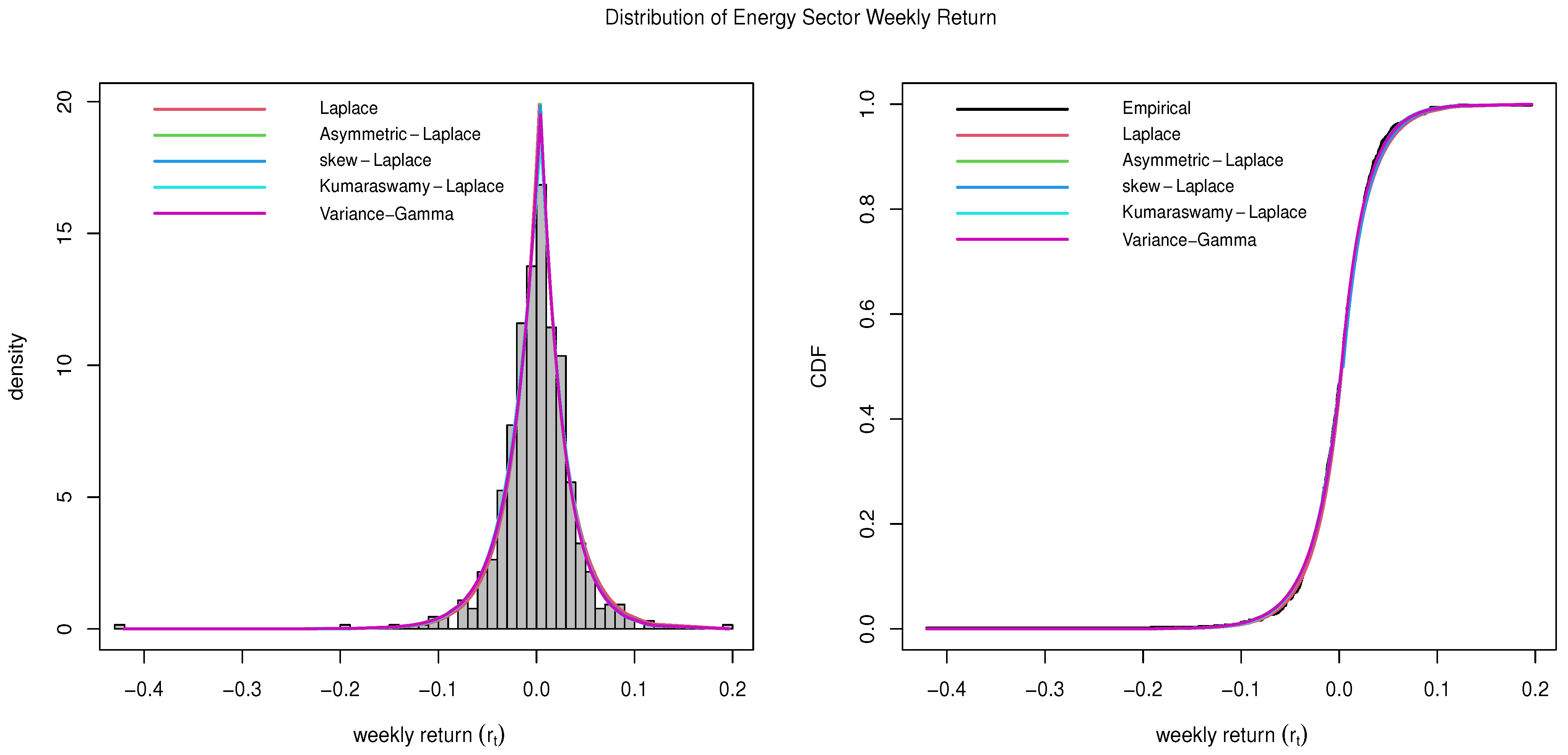
The Energy Sector comprises businesses involved in the exploration, production, refining, and sale of energy resources, including oil and natural gas, as well as companies that service these industries. The energy sector includes some of the largest energy companies in the world, such as Exxon Mobil (XOM) and Chevron (CVX). The Energy Sector achieved a 5.95% annualized return in the last 10 years, and it is known as the best performer sector of S&P 500 in the years 2021 and 2022 (Lazy Portfolio 2023).

The estimated parameters and the goodness-of-fit statistics, including the KS-test statistics (D) for the Energy Sector data, are provided in

Table 4. Estimated parameters and goodness-of-fit statistics: Energy Sector.

Distribution	Parameters	Log-Likelihood	AIC	KS-Test
Laplace	$\mu =0.0030,\sigma =0.0251$	1287.874	−2571.748	$0.0358$
				$\left(0.3774\right)$
Asy. Laplace	$\mu =0.0041,\sigma =0.0125$	1290.349	$-2574.698$	$0.0329$
	$p=0.5349$			$\left(0.4863\right)$
Skew Laplace	$\mu =0.0041,\sigma =0.0252$	1290.233	$-2574.466$	$0.0391$
	$\lambda =-0.0582$			$\left(0.2746\right)$
Kum-Laplace	$\mu =0.0044,\sigma =0.0334$	1290.459	$-2572.918$	$0.0212$
	$a=1.3314$, $b=1.5333$			$\left(0.9328\right)$
Variance-Gamma	$c=0.0042$, $\sigma =0.0352$	1290.368	$-2572.736$	$0.0248$
	$\theta =-0.0036$, $\nu =0.9708$			$\left(0.8204\right)$

. The number in the parenthesis in the KS-test column is the p-value of the test. The plots comparing all five distributions described in Section 2 are given in Figure 2. It is evident that all five distributions fit well with the subject data. Specifically, Kumaraswamy Laplace also has a slight edge over the Variance-Gamma distribution for the subject data.

4.3. Consumer Discretionary Sector

The Consumer Discretionary Sector, also known as consumer cyclical, encompasses companies engaged in retail, eCommerce, hotel, luxury goods, leisure, and travel industries. Unlike consumer staples, these goods and services are often considered non-essential or discretionary purchases. Some of the major players within this sector include Amazon (AMZN), Tesla (TSLA), and Home Depot (HD). Over the last decade, the Consumer Discretionary Sector has delivered an impressive annualized return of 11.91% in the last 10 years (Lazy Portfolio 2023), showcasing its resilience and growth potential in the market. This sector’s performance underscores its importance in reflecting consumer sentiment, economic trends, and evolving consumer preferences. As consumer behavior continues to evolve, driven by technological advancements and changing lifestyles, the Consumer Discretionary Sector remains dynamic and poised for further growth opportunities.

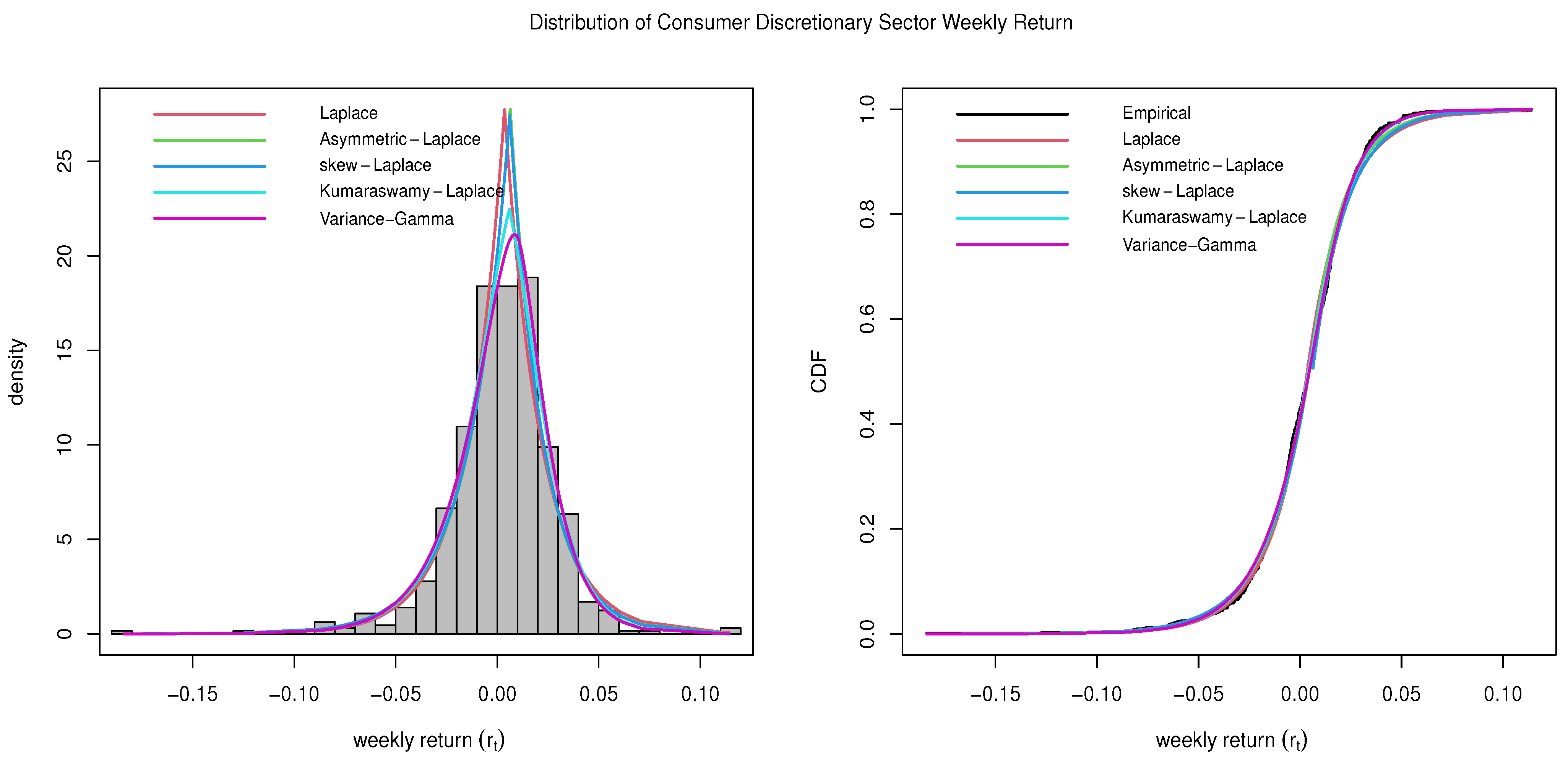
The estimated parameters and the goodness-of-fit statistics, including the KS-test statistics (D) for the Consumer Discretionary Sector data, are provided in

Table 5. Estimated parameters and goodness-of-fit statistics: Cons. Discretionary Sector.

Distribution	Parameters	Log-Likelihood	AIC	KS-Test
Laplace	$\mu =0.0036$, $\sigma =0.0180$	1502.377	−3000.754	$0.0500$
				$\left(0.0784\right)$
Asy. Laplace	$\mu =0.0064$,$\sigma =0.0089$	$1504.738$	$-3000.476$	$0.0489$
	$p=0.5511$			$\left(0.0903\right)$
Skew Laplace	$\mu =0.0062$,$\sigma =0.0182$	$1505.220$	$-3004.440$	$0.0502$
	$\lambda =-0.0895$			$\left(0.0765\right)$
Kum-Laplace	$\mu =0.0060$, $\sigma =0.0492$	1512.373	$-3016.746$	$0.0311$
	$a=2.8722$, $b=5.3012$			$\left(0.5593\right)$
Variance-Gamma	$c=0.0105$,$\sigma =0.0235$	1512.663	$-3017.326$	$0.0256$
	$\theta =-0.0080$, $\nu =0.5386$			$\left(0.7904\right)$

. The number in the parenthesis in the KS-test column is the p-value of the test. The plots comparing all five distributions described in Section 2 are given in Figure 3.

It can be observed that Variance-Gamma seems to be a slightly better fit than other distributions. However, the Kumaraswamy Laplace distribution also fits equally well.

4.4. Consumer Staples Sector

The Consumer Staples Sector includes companies involved in food, beverages, and tobacco, as well as the producers of household goods and personal products. Since these are goods and services that consumers need, regardless of their current financial condition, consumer staples are considered to be a defensive sector (i.e., recession-proof industries). The largest Consumer Staples companies include Walmart (WMT), Procter & Gamble (PG), and The Coca-Cola Company (KO). The Consumer Staples Sector delivered a 10.76% annualized return in the last 10 years (Lazy Portfolio 2023).

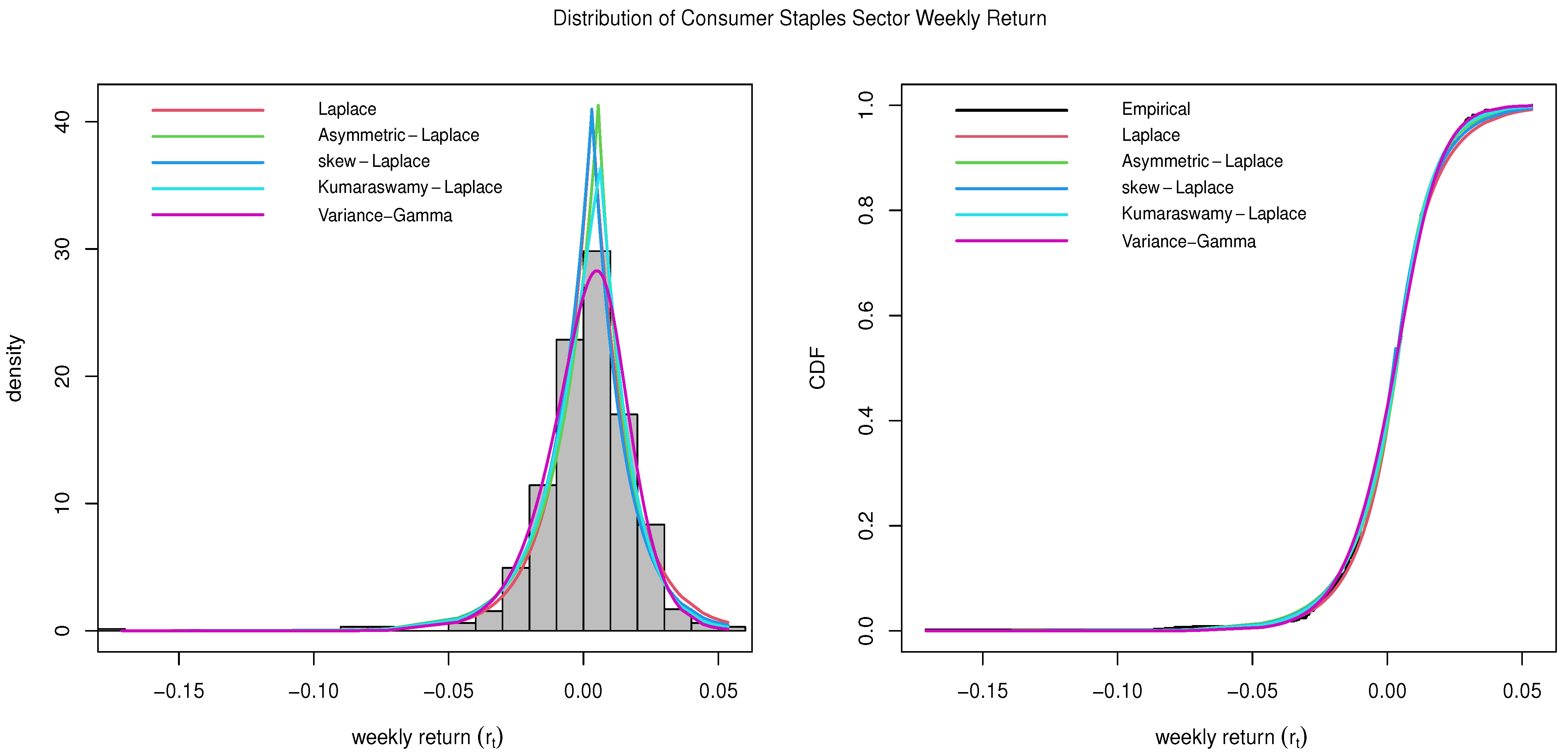
The estimated parameters and the goodness-of-fit statistics, including the KS-test statistics (D) for the Consumer Staples sector data, are provided in

Table 6. Estimated parameters and goodness-of-fit statistics: Cons. Staples Sector.

Distribution	Parameters	Log-Likelihood	AIC	KS-Test
Laplace	$\mu =0.0031$, $\sigma =0.0122$	$1755.652$	$-3507.304$	$0.0372$
				$\left(0.3321\right)$
Asy. Laplace	$\mu =0.0055,\sigma =0.0059$	1763.589	$-3521.178$	$0.0338$
	$p=0.5786$			$\left(0.4496\right)$
Skew Laplace	$\mu =0.0031,\sigma =0.0122$	1758.612	$-3511.224$	$0.0405$
	$\lambda =-0.0695$			$\left(0.2390\right)$
Kum-Laplace	$\mu =0.0063,\sigma =0.0195$	1766.554	$-3525.108$	$0.0194$
	$a=1.5573$, $b=2.2421$			$\left(0.9675\right)$
Variance-Gamma	$c=0.0094,\sigma =0.0154$	1758.131	$-3508.262$	$0.0291$
	$\theta =-0.0078$, $\nu =0.2978$			$\left(0.6454\right)$

. The number in the parenthesis in the KS-test column is the p-value of the test. The plots comparing all five distributions described in Section 2 are given in Figure 4. Specifically, Kumaraswamy Laplace also outperforms the Variance-Gamma distribution for the subject data.

4.5. Financial Sector

The financial sector includes a wide range of financial companies, including investment banks, commercial banks, insurance companies, financial service providers, asset management companies, financial brokers, etc. The financial sector includes some of the largest financial companies in the world like Visa (V), JPMorgan Chase (JPM), and Bank of America (BAC). The Financial Sector delivered a 12.01% annualized return in the last 10 years (Lazy Portfolio 2023).

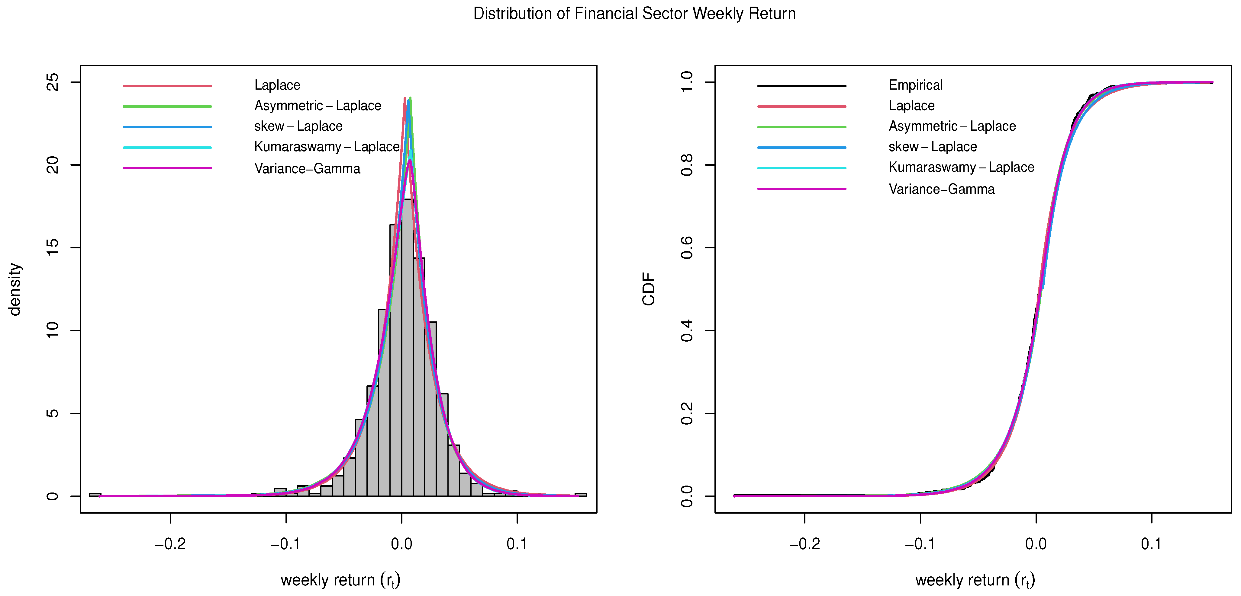
The estimated parameters and the goodness-of-fit statistics, including the KS-test statistics (D) for the Financial Sector data, are provided in

Table 7. Estimated parameters and goodness-of-fit statistics: Financial Sector.

Distribution	Parameters	Log-Likelihood	AIC	KS-Test
Laplace	$\mu =0.0028,\sigma =0.0208$	1408.804	−2813.608	$0.0342$
				$\left(0.4358\right)$
Asy. Laplace	$\mu =0.0075,\sigma =0.0102$	1412.322	$-2818.644$	$0.0399$
	$p=0.5675$			$\left(0.2552\right)$
Skew Laplace	$\mu =0.0058,\sigma =0.0209$	1411.620	$-2817.240$	$0.0440$
	$\lambda =-0.0788$			$\left(0.1624\right)$
Kum-Laplace	$\mu =0.0078,\sigma =0.0367$	1414.784	$-2821.568$	$0.0204$
	$a=1.7552,b=2.4667$			$\left(0.9497\right)$
Variance-Gamma	$c=0.0074,\sigma =0.0281$	1414.534	$-2821.068$	$0.0228$
	$\theta =-0.0056,\nu =0.7351$			$\left(0.8894\right)$

. The number in the parenthesis in the KS-test column is the p-value of the test. The plots comparing all five distributions described in Section 2 are given in Figure 5. The Kumaraswamy Laplace distributions outperform the other generalized Laplace distributions. It also has a slight edge over the Variance-Gamma distribution for the subject data.

4.6. Healthcare Sector

The Healthcare Sector consists of the stocks of companies involved in a range of health-related industries, including but not limited to pharmaceutical producers, medical devices, healthcare service providers, biotech stocks, insurance companies, etc. Examples of large healthcare companies include UnitedHealth Group (UNH) and Pfizer (PFE). The Healthcare Sector delivered a 14.85% annualized return in the last 10 years, and is known as the second-best performer sector of S&P 500 only after the Information Technology Sector (Lazy Portfolio 2023).

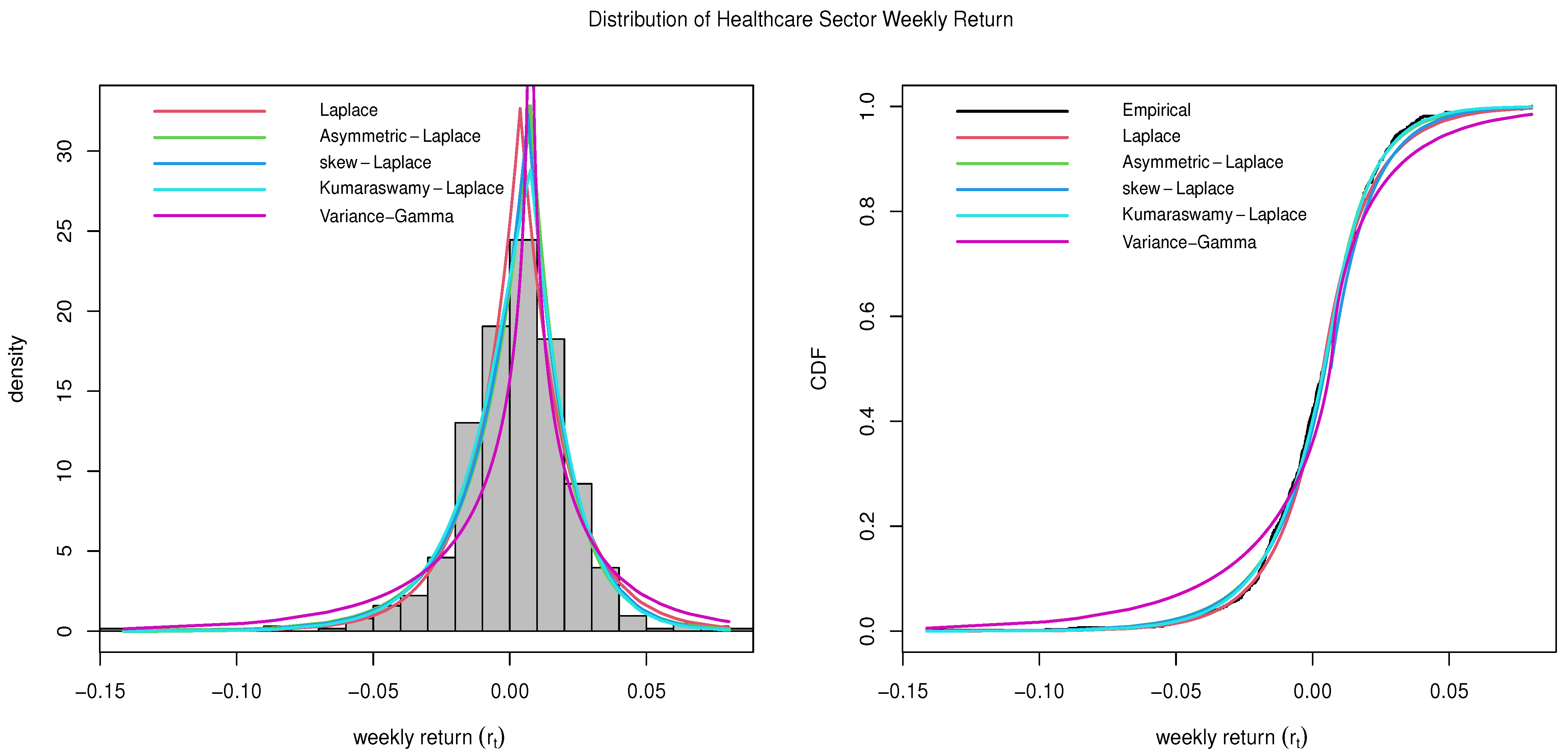
The estimated parameters and the goodness-of-fit statistics, including the KS-test statistics (D) for the Healthcare Sector data, are provided in

Table 8. Estimated parameters and goodness-of-fit statistics: Healthcare Sector.

Distribution	Parameters	Log-Likelihood	AIC	KS-Test
Laplace	$\mu =0.0038,\sigma =0.0153$	1564.960	−3125.920	$0.0402$
				$\left(0.2605\right)$
Asy. Laplace	$\mu =0.0074,\sigma =0.0074$	1572.279	$-3138.558$	$0.0403$
	$p=0.5841$			$\left(0.2595\right)$
Skew Laplace	$\mu =0.0067,\sigma =0.0155$	1572.160	$-3138.320$	$0.0696$
	$\lambda =-0.1172$			$\left(0.0045\right)$
Kum-Laplace	$\mu =0.0076,\sigma =0.0251$	1575.184	$-3142.368$	$0.0204$
	$a=1.6091$, $b=2.2829$			$\left(0.8521\right)$
Variance-Gamma	$c=0.0076,\sigma =0.0343$	$1515.385$	$-3022.770$	$0.0774$
	$\theta =-0.0060$,$\nu =2.1546$			$\left(0.0011\right)$

. The number in the parenthesis in the KS-test column is the p-value of the test. The plots comparing all five distributions described in Section 2 are given in Figure 6. It can be observed that the Kumaraswamy Laplace distribution outperforms all other generalizations of the Laplace family. It also outperforms the Variance-Gamma distribution for the subject data.

4.7. Industrials Sector

The Industrials Sector may include businesses that are involved in a wide range of industries, including industrial machinery construction and engineering, aerospace and defense, electrical equipment, etc. Some of the largest industrial companies in the world include Boeing (BA), Honeywell (HON), and Union Pacific (UNP). The Industrials Sector delivered a 12.11% annualized return in the last 10 years (Lazy Portfolio 2023).

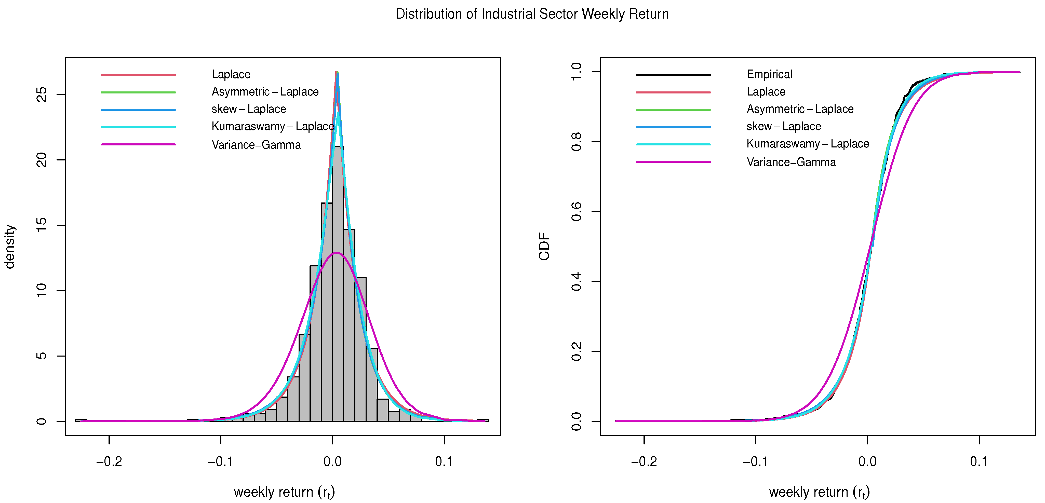
The estimated parameters and the goodness-of-fit statistics, including the KS-test statistics (D) for the Industrial Sector data, are provided in

Table 9. Estimated parameters and goodness-of-fit statistics: Industrials Sector.

Distribution	Parameters	Log-Likelihood	AIC	KS-Test
Laplace	$\mu =0.0033,\sigma =0.0187$	1477.463	−2950.926	$0.0344$
				$\left(0.4275\right)$
Asy. Laplace	$\mu =0.0046,\sigma =0.0093$	1479.421	$-2952.842$	$0.0349$
	$p=0.5360$			$\left(0.4074\right)$
Skew Laplace	$\mu =0.0046,\sigma =0.0188$	1479.536	$-2953.072$	$0.0361$
	$\lambda =-0.0664$			$\left(0.3673\right)$
Kum-Laplace	$\mu =0.0050,\sigma =0.0312$	1481.504	$-2955.008$	$0.0273$
	$a=1.7082$, $b=2.1339$			$\left(0.7221\right)$
Variance-Gamma	$c=0.0121,\sigma =0.0322$	1424.007	$-2840.014$	$0.1013$
	$\theta =-0.0103,\nu =0.1184$			$\left(0.0001\right)$

. The number in the parenthesis in the KS-test column is the p-value of the test. The plots comparing all five distributions described in Section 2 are given in Figure 7. It can be observed that the Kumaraswamy Laplace distribution outperforms all other generalizations of the Laplace distribution. It also outperforms the Variance-Gamma distribution for the subject data.

4.8. Information Technology Sector

The Information Technology (IT) Sector includes multiple sub-sectors and industries, from semiconductor producers to software and hardware providers, as well as internet stocks and cloud computing. The sector includes companies with some of the largest market capitalizations in the world, such as Apple (AAPL), Microsoft (MSFT), Accenture Plc (ACN), Meta Platforms, Inc (META), etc. It had a 17.46% annualized return in the last 10 years, and is known as the best performer sector of S&P 500 over the past 10 years (Lazy Portfolio 2023).

The estimated parameters and the goodness-of-fit statistics, including the KS-test statistics (D) for the Information Technology Sector data, are provided in

Table 10. Estimated parameters and goodness-of-fit statistics: IT Sector.

Distribution	Parameters	Log-Likelihood	AIC	KS-Test
Laplace	$\mu =0.0051,\sigma =0.0186$	1482.902	−2961.804	$0.0323$
				$\left(0.5077\right)$
Asy. Laplace	$\mu =0.0096,\sigma =0.0089$	1492.046	$-2978.092$	$0.0317$
	$p=0.5907$			$\left(0.5332\right)$
Skew Laplace	$\mu =0.0051,\sigma =0.0186$	1485.442	$-2964.884$	$0.0209$
	$\lambda =-0.0629$			$\left(0.2726\right)$
Kum-Laplace	$\mu =0.0106,\sigma =0.0313$	1492.893	$-2977.786$	$0.0208$
	$a=1.6333,b=2.4462$			$\left(0.9423\right)$
Variance–Gamma	$c=0.0096,\sigma =0.0427$	1437.612	$-2867.224$	$0.06811$
	$\theta =-0.0072,\nu =2.0281$			$\left(0.0049\right)$

. The number in the parenthesis in the KS-test column is the p-value of the test. The plots comparing all five distributions described in Section 2 are given in Figure 8. Note that the Kumaraswamy Laplace distribution fits the data better than other generalizations of Laplace distribution. It also outperforms the Variance-Gamma distribution for the subject data.

4.9. Materials Sector

The Materials Sector includes businesses involved in the manufacture of construction materials, chemicals, paper, glass, companies specializing in making paper and forest products metals, and mining companies. Some of the largest materials companies in the world include DuPont (DD) and The Sherwin-Williams Company (SHW). The Materials Sector delivered a 9.78% annualized return in the last 10 years (Lazy Portfolio 2023).

The estimated parameters and the goodness-of-fit statistics, including the KS-test statistics (D) for the Materials Sector data, are provided in

Table 11. Estimated parameters and goodness-of-fit statistics: Materials Sector.

Distribution	Parameters	Log-Likelihood	AIC	KS-Test
Laplace	$\mu =0.0017,\sigma =0.0207$	1412.930	−2821.860	$0.0341$
				$\left(0.4384\right)$
Asy. Laplace	$\mu =0.0019,\sigma =0.0104$	1412.963	$-2819.926$	$0.0325$
	$p=0.5026$			$\left(0.5018\right)$
Skew Laplace	$\mu =0.0026,\sigma =0.0207$	1413.102	$-2820.204$	$0.0209$
	$\lambda =-0.0265$			$\left(0.9405\right)$
Kum-Laplace	$\mu =0.0016$, $\sigma =0.0376$	1415.617	$-2823.234$	$0.0208$
	$a=1.9667$,$b=2.2985$			$\left(0.9423\right)$
Variance-Gamma	$c=0.0216,\sigma =0.0776$	1032.473	$-2056.946$	$0.2476$
	$\theta =-0.0193,\nu =0.1184$			$\left(0.0001\right)$

. The plots comparing all five distributions described in Section 2 are given in Figure 9. Note that Laplace distribution and its generalizations fit better than the Variance-Gamma distribution for the Materials Sector data. The Kumaraswamy Laplace outperforms the rest of the other distributions within the Laplace family.

4.10. Real Estate Sector

The Real Estate Sector includes companies that develop or manage real estate property. This sector also includes real estate investment trusts (REITS), which are companies that purchase multiple income-producing assets, such as office buildings and hotels. Some of the largest real estate companies include American Tower Corp. (AMT) and Simon Property Group (SPG). The Real Estate Sector delivered a 7.42% annualized return in the last 10 years (Lazy Portfolio 2023).

The estimated parameters and the goodness-of-fit statistics, including the KS-test statistics (D) for the Real Estate Sector data, are provided in

Table 12. Estimated parameters and goodness-of-fit statistics: Real Estate Sector.

Distribution	Parameters	Log-Likelihood	AIC	KS-Test
Laplace	$\mu =0.0031,\sigma =0.0188$	1474.430	−2944.860	$0.0341$
				$\left(0.4717\right)$
Asy. Laplace	$\mu =0.0062,\sigma =0.0092$	1477.283	$-2948.566$	$0.0296$
	$p=0.5609$			$\left(0.6216\right)$
Skew Laplace	$\mu =0.0043,\sigma =0.0189$	1476.053	$-2946.106$	$0.0243$
	$\lambda =-0.0519$			$\left(0.8390\right)$
Kum-Laplace	$\mu =0.0063,\sigma =0.0318$	1477.655	$-2947.310$	$0.0231$
	$a=1.6941,b=2.2528$			$\left(0.8814\right)$
Variance–Gamma	$c=0.0116,\sigma =0.0375$	1376.423	$-2744.846$	$01369$
	$\theta =-0.0086,\nu =0.1184$			$\left(0.0001\right)$

. The plots comparing all five distributions described in Section 2 are given in Figure 10. It can be observed that the Laplace distribution and its generalizations fit better than the Variance-Gamma distribution for the Real Estate Sector data. The Kumaraswamy Laplace outperforms the rest of the other distributions within the Laplace family.

4.11. Utilities Sector

The Utilities Sector includes companies that provide customers with utility services, such as water, electricity, and gas. Since utilities are considered to be essentials for daily living, the utility sector is also generally seen as a defensive sector. Some of the largest utility companies include NextEra Energy (NEE), Duke (DUK), and The Southern Company (SO). The Utility Sector delivered a 10.87% annualized return in the last 10 years (Lazy Portfolio 2023).

The estimated parameters and the goodness-of-fit statistics, including the KS-test statistics (D) for the Utilities Sector data, are provided in

Table 13. Estimated parameters and goodness-of-fit statistics: Utilities Sector.

Distribution	Parameters	Log-Likelihood	AIC	KS-Test
Laplace	$\mu =0.0028,\sigma =0.0157$	1593.560	−3183.120	$0.0429$
				$\left(0.1843\right)$
Asy. Laplace	$\mu =0.0065,\sigma =0.0076$	1598.980	$-3191.960$	$0.0356$
	$p=0.5815$			$\left(0.3842\right)$
Skew Laplace	$\mu =0.0044,\sigma =0.0157$	1597.486	$-3188.972$	$0.0409$
	$\lambda =-0.0747$			$\left(0.2277\right)$
Kum-Laplace	$\mu =0.0084,\sigma =0.0246$	1604.116	$-3200.232$	$0.0274$
	$a=1.4908,b=2.2459$			$\left(0.7166\right)$
Variance–Gamma	$c=0.0044,\sigma =0.0358$	1549.869	$-3091.738$	$0.0790$
	$\theta =-0.0032,\nu =2.0000$			$\left(0.0006\right)$

. The plots comparing all five distributions described in Section 2 are given in Figure 11. It can be observed that the Laplace distribution and its generalizations fit better than the Variance-Gamma distribution for the Utilities Sector data. In particular, the Kumaraswamy Laplace outperforms the other competing distributions.

4.12. S&P 500 Index

The first S&P Index was launched in 1923 as a joint project by the Standard Statistical Bureau and Poor’s Publishing. The original index covered 233 companies in 26 different industries. The two companies merged in 1941 to become Standard and Poor’s. The Standard and Poor’s 500, or simply the S&P 500, is a stock market index tracking the stock performance of 500 large companies listed on stock exchanges in the United States. It is one of the most commonly followed equity indices in the world. As of 31 December 2021, more than USD 7.1 trillion was invested in assets tied to the performance of the index. The S&P 500 index delivered a 12.46% annualized return in the last 10 years (Lazy Portfolio 2023).

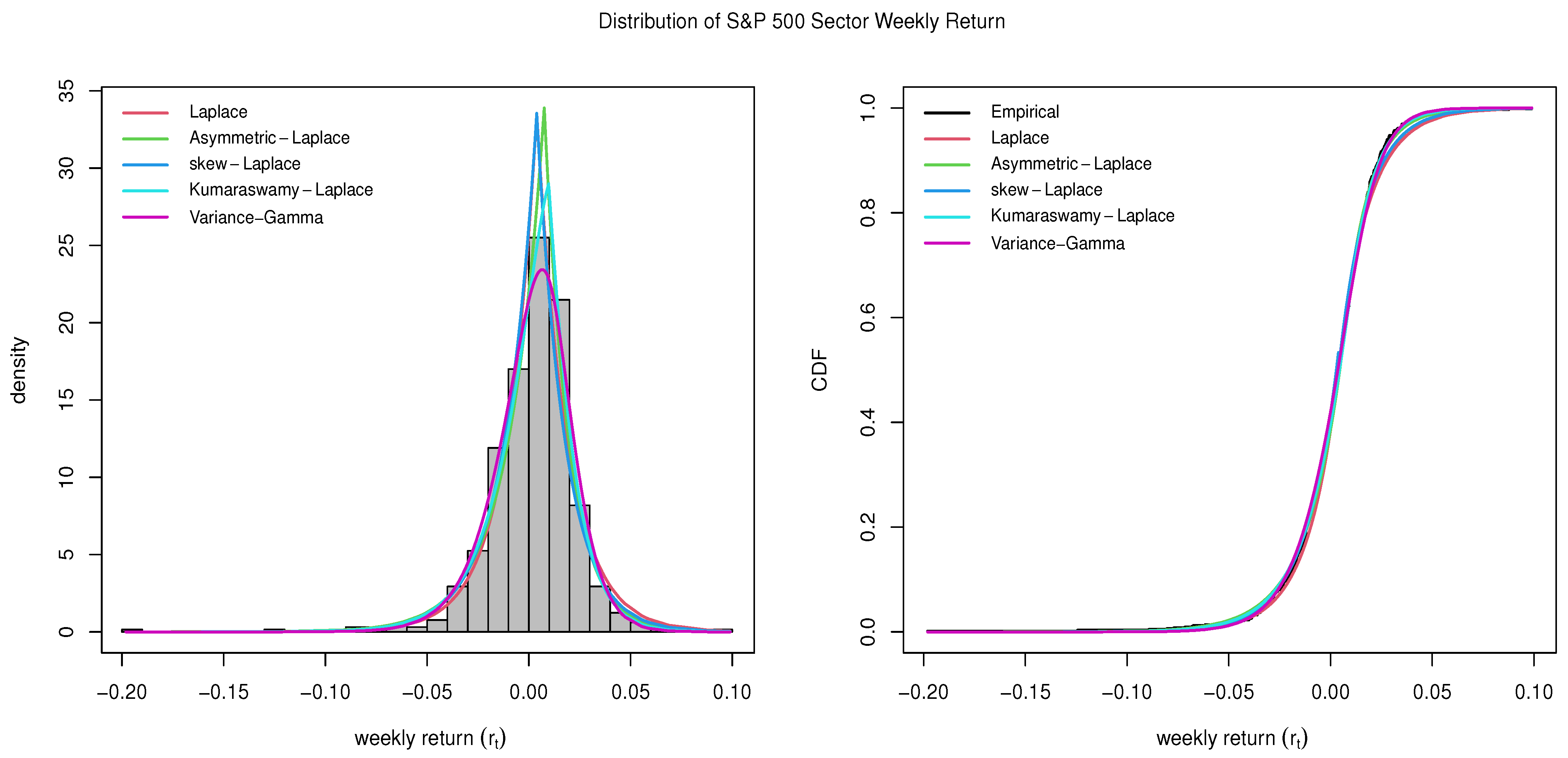
The estimated parameters and the goodness-of-fit statistics for the S&P 500 Index data are provided in

Table 14. Estimated parameters and goodness-of-fit statistics: S&P 500 Index.

Distribution	Parameters	Log-Likelihood	AIC	KS-Test
Laplace	$\mu =0.0039,\sigma =0.0149$	1625.187	-3246.374	$0.0405$
				$\left(0.2376\right)$
Asy. Laplace	$\mu =0.0076,\sigma =0.0071$	1633.946	$-3261.892$	$0.0228$
	$p=0.5947$			$\left(0.8885\right)$
Skew Laplace	$\mu =0.0039,\sigma =0.0149$	1628.095	$-3250.190$	$0.0409$
	$\lambda =-0.0630$			$\left(0.2277\right)$
Kum-Laplace	$\mu =0.0098,\sigma =0.0241$	1635.519	$-3263.083$	$0.0274$
	$a=1.5227,b=2.4292$			$\left(0.9061\right)$
Variance–Gamma	$c=0.0116,\sigma =0.0188$	1623.680	$-3239.360$	$0.0315$
	$\theta =-0.0095,\nu =0.3288$			$\left(0.5404\right)$

. The plots comparing all five distributions described in Section 2 are given in Figure 12. It can be observed that a generalized Laplace distribution fits better than the Variance-Gamma distribution to model the S& P Index data.

5. Ranking Probability Distributions for Modeling Stock Returns

It would be ideal if one could discover the probability distribution that universally fits all types of asset returns. However, practically, it is hard to find such one universal distribution that can explain the probabilistic characteristics of various types of asset returns. In this empirical study, we examined the goodness-of-fit of the five popular Laplace family probability distributions among various stock indices of S&P 500 based on p-value criteria. We discovered that out of five distributions, only two of them, namely, Laplace (two parameters) and the Kumaraswamy Laplace (four parameters) distributions, fit the returns data from all eleven indices, including the benchmark index S&P 500. Our main objective of this study is to compare the performance of the four-parameter probability distributions: the popular Variance-Gamma with Laplace distribution and its generalizations. It is interesting to note that in eleven out of twelve indices, Kumaraswamy Laplace (Kum-Laplace) outperforms the VG distribution, except for the Consumer Discretionary index.

Table 15. Rank of goodness-of-fit of the distribution based on KS p-values.

Index	Distribution	KS p-Value	Fail to Reject ${\mathit{H}}_0$?	Rank
Communication Service	Kum-Laplace	$0.2308$	Yes	1
	Laplace	0.1067	Yes	2
	Asy. Laplace	0.0709	Yes	3
	Skew Laplace	0.0001	No	4
	Variance-Gamma	0.0001	No	5
Energy	Kum-Laplace	$0.9328$	Yes	1
	Variance-Gamma	0.8204	Yes	2
	Asy. Laplace	0.4863	Yes	3
	Laplace	0.3774	Yes	4
	Skew Laplace	0.2746	Yes	5
Consumer Discretionary	Variance-Gamma	0.7904	Yes	1
	Kum-Laplace	0.5593	Yes	2
	Asy. Laplace	0.0903	Yes	3
	Laplace	0.0784	Yes	4
	Skew Laplace	0.0765	Yes	5
Consumer Staples	Kum-Laplace	0.9675	Yes	1
	Variance-Gamma	0.6454	Yes	2
	Asy. Laplace	0.4496	Yes	3
	Laplace	0.2390	Yes	4
	Skew Laplace	0.3321	Yes	5
Financials	Kum-Laplace	0.9497	Yes	1
	Variance-Gamma	0.8894	Yes	2
	Laplace	0.4358	Yes	3
	Asy. Laplace	0.2552	Yes	4
	Skew Laplace	0.0162	No	5
Healthcare	Kum-Laplace	0.8521	Yes	1
	Asy. Laplace	0.2595	Yes	2
	Laplace	0.2605	Yes	3
	Skew Laplace	0.0045	No	4
	Variance-Gamma	0.0011	No	5

and

Table 16. Rank of goodness-of-fit of the distribution based on KS p-values (continued).

Index	Distribution	KS p-Value	Fail to Reject ${\mathit{H}}_0$?	Rank
Industrials	Kum-Laplace	0.7221	Yes	1
	Laplace	0.4275	Yes	2
	Asy. Laplace	0.4074	Yes	3
	Skew Laplace	0.3673	Yes	4
	Variance-Gamma	0.0001	No	5
Information Technology	Kum-Laplace	0.9423	Yes	1
	Asy. Laplace	0.5332	Yes	2
	Laplace	0.5077	Yes	3
	Skew Laplace	0.2726	Yes	4
	Variance-Gamma	0.0049	No	5
Materials	Kum-Laplace	0.9423	Yes	1
	Skew Laplace	0.9405	Yes	2
	Asy. Laplace	0.5018	Yes	3
	Laplace	0.4384	Yes	4
	Variance-Gamma	0.0001	No	5
Real Estate Sector	Kum-Laplace	0.8814	Yes	1
	Skew Laplace	0.8390	Yes	2
	Asy. Laplace	0.6216	Yes	3
	Laplace	0.4717	Yes	4
	Variance-Gamma	0.0001	No	5
Utilities Sector	Kum-Laplace	0.7166	Yes	1
	Asy. Laplace	0.3842	Yes	2
	Skew Laplace	0.2277	Yes	3
	Laplace	0.1843	Yes	4
	Variance-Gamma	0.0006	No	5
S&P 500 Index	Kum-Laplace	0.9061	Yes	1
	Asy. Laplace	0.8885	Yes	2
	Variance-Gamma	0.5404	Yes	3
	Laplace	0.2376	Yes	4
	Skew Laplace	0.2277	Yes	5

provide the ranking of the most appropriate distribution to model index returns data based on Kolmogorov–Smirnov (K-S) p-value criteria. The null hypothesis of the subject of study is that the returns data follows a specified distribution, whereas the alternative hypothesis says otherwise.

The rank of the specified distribution is 1 through 5, where Rank 1 refers to the most appropriate and Rank 5 is the least appropriate distribution for index returns modeling. The distributions without rank are not appropriate for modeling returns datasets from the specified index in a given period. It is found that Kumaraswamy Laplace distribution is the number one probability distribution among the Laplace family of distributions, and the Variance-Gamma distribution fails measurably, especially for Communication Services, Healthcare, Industrial, Information Technology, Materials, Real Estate, and Utilities sectors of S&P 500. The rank of the distributions provides very useful information for financial analysts concerning their application in modeling returns, while the correct choice of the distribution for modeling leads to excellence in prediction.

6. Exceedance Probability Prediction

The exceedance probability is the probability of a random variable exceeding a certain threshold. The complement of exceedance probability is often called the non-exceedance probability. Based on the choice of probability distribution, we may obtain a different exceedance probability. In

Table 17. Exceedance Probability for S&P 500 Index.

Return Level (%)	0	0.01	0.02	0.03	0.04	0.05
Observed Probability	0.604	0.349	0.135	0.053	0.023	0.011
Laplace	0.615	0.332	0.169	0.087	0.044	0.023
Bias	−0.011	0.017	−0.034	−0.034	−0.021	−0.012
Asy. Laplace	0.615	0.332	0.144	0.062	0.027	0.012
Bias	−0.011	0.017	−0.009	−0.009	−0.004	−0.001
Skew Laplace	0.582	0.323	0.158	0.077	0.037	0.018
Bias	0.022	0.026	−0.023	−0.024	−0.014	−0.007
Kum-Laplace	0.604	0.348	0.146	0.058	0.022	0.008
Bias	0.000	0.001	−0.011	−0.005	0.001	0.003
Variance-Gamma	0.580	0.351	0.159	0.059	0.019	0.006
Bias	0.024	−0.002	−0.024	−0.006	0.004	0.005

, we present the exceedance probability at different return levels of the S&P data using the distributions discussed in Section 2.

We can see from Table 17 that Kumaraswamy Laplace has a low bias as compared to the Variance-Gamma distribution while predicting the exceedance probability of different return levels of S&P 500. These findings also attest that Kum-Laplace outperforms VG distribution while fitting returns data. One can compute the exceedance probability of all eleven business segments.

7. Parallel Inferences and Discussions

We expanded our empirical investigations to assess the goodness-of-fit of all five chosen probability distributions on returns from stock indices across both emerging and developed markets. Our analysis focused on the IBOVESPA from Brazil and the KOSPI from Korea, spanning from January 2010 to May 2022 and encompassing daily, weekly, and monthly stock returns data. Consistently, our findings underscore the superior fit of the Kumaraswamy Laplace distribution compared to the other distributions examined. This trend persisted when the distribution was applied to various assets, such as the 20+ Year Treasury Bond ETF (TLT), as well as prominent individual stocks like Amazon and Apple. Specifically, when examining the KOSPI index on a daily, weekly, and monthly basis, we found KS statistics p-values of 0.6130, 0.8885, and 0.9687, respectively. Likewise, for the IBOVESPA index, the p-values for KS statistics were 0.6308, 0.5577, and 0.9448, corresponding to the daily, weekly, and monthly stock index returns dataset, respectively. Similarly, for individual stocks Amazon and Apple, the p-values over daily, weekly, and monthly were (0.5327 and 0.1848), (0.8096 and 0.7015), and (0.8084 and 0.2919), respectively. For the 20+ Year Treasury Bond ETF (TLT), based on available weekly and monthly data, KS statistics p-values were 0.2965 and 0.3228. Additionally, our study involved calculating log-likelihood functions and goodness-of-fit statistics, consistently favoring the Kumaraswamy Laplace distribution over other competitive distributions considered.

The empirical evidence across diverse markets, asset classes, and timeframes reaffirms the superiority of the Kumaraswamy Laplace distribution in modeling stock returns data. Consequently, it emerges as a robust alternative to other Laplace family distributions, including the Variance-Gamma distribution.

Probability distributions play a pivotal role in modeling potential returns within asset portfolios. The Kumaraswamy Laplace distribution (Kum-Laplace) offers a powerful tool for enhancing portfolio construction and risk analysis. By employing this distribution, investors can effectively model the distribution of portfolio returns, amalgamating individual asset return distributions for comprehensive evaluations of expected returns and inherent variability (risk). Furthermore, the Kum-Laplace distribution facilitates the computation of various risk metrics, including standard deviation, value-at-risk (VaR), and conditional value-at-risk (CVaR), thereby providing valuable insights into portfolio downside risk exposure across a spectrum of probability scenarios.

Furthermore, probability distributions seamlessly integrate into portfolio optimization models, allowing for the creation of portfolios that maximize returns while maintaining predetermined risk levels or minimize risk while targeting specific return levels. Modern portfolio theory serves as a prime example, leveraging probability distributions to identify optimal asset allocations within portfolios. Consequently, the Kum-Laplace probability distribution offers a robust framework for understanding uncertainty in financial markets, empowering investors to make informed decisions regarding portfolio construction and risk management.

8. Concluding Remarks

Modeling and predicting stock returns are pivotal tasks in the financial market, offering investors valuable guidance to mitigate risks in their portfolio management. The Laplace distribution has emerged as a favored alternative to the normal variance model, owing to its adept fit with financial data and its effective portrayal of underlying behaviors. However, the quest for a universal distribution capable of fitting all forms of financial data proves virtually unattainable, particularly when dealing with complex natural phenomena like stock returns. In this context, both Laplace and generalized Laplace probability distributions play crucial roles in modeling asset returns. The four-parameter Variance-Gamma distribution stands out as the preferred choice for modeling stock returns, extensively examined in finance and economics literature.

In this article, we conducted an empirical investigation using real market data from the S&P 500 index and its eleven business sector indices, employing Laplace distributions and their generalized forms, which encompass both the four-parameter Variance Gamma and the Kumaraswamy Laplace distribution. Additionally, we evaluated the goodness-of-fit of these distributions on returns across various assets class, investment durations, and market types, including 20+ Years Treasury Bond ETFs, individual stocks, and international stock indices such as IBOVESPA and KOSPI.

Our analysis indicates that the Kumaraswamy Laplace distribution is the only distribution consistently fitting stock/index returns data across diverse assets class, investment durations, and market types. Given the compelling evidence presented, the superior performance of the Kumaraswamy Laplace distribution over other choices establishes, it as a robust alternative for practitioners aiming for precise return predictions and efficient risk mitigation in their investments.