Article

A Deep Learning Approach to Dynamic Interbank Network Link Prediction

The Institute for Financial Services Analytics, University of Delaware, Newark, DE 19716, USA
Int. J. Financial Stud. 2022, 10(3), 54; https://doi.org/10.3390/ijfs10030054
Submission received: 25 May 2022 / Revised: 6 July 2022 / Accepted: 7 July 2022 / Published: 12 July 2022
(This article belongs to the Special Issue Financial Econometrics and Machine Learning)

Abstract

:
Lehman Brothers’ failure in 2008 demonstrated the importance of understanding interconnectedness in interbank networks. The interbank market plays a significant role in facilitating market liquidity and providing short-term funding for each other to smooth liquidity shortages. Knowing the trading relationship could also help understand risk contagion among banks. Therefore, future lending relationship prediction is important to understand the dynamic evolution of interbank networks. To achieve the goal, we apply a deep learning framework model of interbank lending to an electronic trading interbank network for temporal trading relationship prediction. There are two important components of the model, which are the Graph convolutional network (GCN) and the Long short-term memory (LSTM) model. The GCN and LSTM components together capture the spatial–temporal information of the dynamic network snapshots. Compared with the Discrete autoregressive model and Dynamic latent space model, our proposed model achieves better performance in both the precrisis and the crisis period.

1. Introduction

Interbank lending networks are of great practical importance in that the ability and willingness of banks to provide short-term funding for each other (with banks that temporarily have less cash than needed to support their business operations borrowing from banks that temporarily have more cash than needed) is crucial to the real economy. As emphasized by Hatzopoulos et al. (2015), a robust interbank market could help the central bank achieve its desired interest rate and allow institutions to efficiently trade liquidity. In normal times, interbank markets are among the most liquid in the financial sector. When bank networks freeze up, a sharp decline in transaction volume in this market was a major contributing factor to the collapse of several financial institutions during the financial crisis. The contagion of systemic risk is strongly related to interbank connectedness. Understanding the dynamic interbank connectedness or interbank topology could enhance the understanding of risk contagion.
A large fraction of previous research on interbank connectedness studies static and aggregated interbank networks, which reveals information about long-term connectedness inside a network, while other studies explored the dynamics of the interbank networks. Papers that focus on the static network such as (Gai et al. 2011) discussed how interbank connectedness affects the spread of contagion and the implication for the stability of the banking system. However, Denbee et al. (2021) argued that similar interbank connectedness structures might generate different liquidity transmission outcomes as banks have different strategies when they observe liquidity surplus among neighbors. Therefore, instead of overall interbank connectedness, knowing pairwise future interbank connectedness better smooths temporary liquidity shortages and reduces “funding liquidity risk”. Since bank trading strategies are different in normal and crisis periods, instead of obtaining a long-term static overall connectedness network pattern, a shorter-term pairwise connectedness is more desirable to understand interbank connectedness that drives us to model the interbank network in a dynamic way.
Previous research studies (Bräuning and Fecht 2012; Bräuning and Koopman 2020; Giraitis et al. 2012; Linardi et al. 2020; Mazzarisi et al. 2019) on pairwise dynamic interbank connectedness mostly focus on the underlying mechanisms determining the likelihood of trading with methods such as regression, dynamic latent space model and dynamic factor model. These methods are all statistical-based models with underlying model assumptions. In addition, most of them cooperate with central banks, and data are not accessible for noncentral banks. In addition, complex estimation strategies are applied in these models and special approaches are needed to achieve accurate estimation.
In this paper, we aim to contribute a better understanding of the dynamic of financial interbank networks by applying a deep learning approach to weekly network snapshots in an electronic interbank trading platform called the e-MID market. A detailed explanation of the e-MID market is provided in Section 4. The primary goal of this study is to accurately forecast interbank future lending relationships by proposing a deep learning forecasting model. Two baseline predictive models are also built in this study for comparison with our proposed model. The key contributions of this study are:
  • Inspired by Chen et al. (2021), the model is proposed to combine the advantages of the Graph convolutional network (GCN), which obtains valuable information and learns the internal representations of the network snapshots, with the benefits of the Long short-term memory model (LSTM), which is effective at identifying and modeling short and long-term temporal relationships embedded in the sequence of data.
  • To handle the network sparsity and the fact that we care more about the existing links than nonexisting links; we design a loss function that adds a penalty to nonexisting links.
  • On test data, the proposed model is assessed and compared with two traditional statistical baseline models using the metrics Area Under the ROC Curve (AUC) and Precision–Recall Curve (PRAUC). They are the Discrete autoregressive model and Dynamic latent space model. The findings indicate that our proposed model beats the two models in predicting future links in both precrisis and crisis periods for the top 100 Italian trading dataset and European core countries dataset.
The remaining sections of this manuscript are as follows: Section 2 discusses the key literature that is related to our study, Section 3 studies the methods and model structure, Section 4 shows the main results with different performance metrics and Section 5 summarizes the study and makes a conclusion.

2. Literature Review

This section aims to build the linkage between systemic risk and why we assume that a dynamic link prediction problem is beneficial in better understanding the contagion process. To achieve the goal, two streams of literature are related to the article. The first stream is related to financial contagion and the second stream is related to the methods of understanding dynamic interbank connectedness.

2.1. Financial Contagion

Financial contagion has been widely studied in the past years. Additionally, contagion can take place through a multitude of channels, such as banks run, direct effect such as interbank lending and indirect effect (Upper 2011). To narrow down the scope of the study, we focus on one particular channel, namely direct effects due to losses on interbank loan exposures. Seminal theoretical work by Allen and Gale (2000) provides a starting point for studying a general equilibrium approach to financial market contagion and systemic risk. Together with the work by Freixas et al. (2000), they provide a key insight that the possibility for contagion depends on the structure of the interbank market. Additionally, they both reach a similar conclusion that diversified and completely connected networks are more stable. However, the assumption of a complete network with full risk sharing is not valid in the real world, and the network structures are too simplistic to be sure that the intuitions generated generalize to real-world financial systems. Therefore, researchers study contagion through the simulation process. Using tools of network analysis, the authors found different patterns that make the network prone to contagion. Elliott et al. (2014) found that integration and diversification have different, nonmonotonic effects on the extent of cascades. By using simulated network models, Nier et al. (2007) demonstrates that an increase in connectivity does not necessarily lead to a reduction in systemic risk. Capital and contagion have a negative relationship, suggesting that regulators might prevent contagion with greater capital requirements. Depending on the structure of the network, the shock size has varying effects on a system. Simulations show financial networks have a “robust-yet-fragile tendency”: though the chance of contagion is low, the effects of a problem can be substantial (Gai and Kapadia 2010). Leventides et al. (2019) conclude that heterogeneity in bank sizes and interbank exposures play a significant role in the stability of the financial system since they enhance the system’s ability to absorb shocks. In addition, the degree of interconnectedness of the system has a significant impact on its resilience, particularly in case of smaller and highly interconnected interbank networks.
With the factors that affect the contagion in interbank network stated above, Denbee et al. (2021) argued that banks have different strategies when they observe liquidity surplus among neighbors, despite similar interbank connectedness structures. In this regard, rather than knowing overall interbank connectivity, knowing pairwise future interbank connectivity reduces the risk of funding liquidity shortages by smoothing out temporary liquidity shortages. A dynamic interbank network link prediction model could help understand pairwise future interbank connectivity. In a contagion cascade model, instead of capturing the impact of the hypothetical shock in a static network, we could use the proposed dynamic network link prediction model to predict the network structure of the interbank market to capture some dynamic effects resulting from changing initial conditions which build the relationship between the dynamic link prediction model and financial contagion process.

2.2. Interconnectedness Network Models

With the network models focusing on understanding interbank network formation and interconnectedness, there are two streams of literature we would like to refer to. The first stream is the static network model, and the second stream is the dynamic network model. We start with some potential problems that arise from modeling the interbank network from a static perspective. We then discuss different streams of network modeling literature from static to dynamic extension. To determine the financial stability of the financial network, a simplification of the financial network as static may be helpful in some situations, but understanding the dynamic nature of the financial interbank network is essential. From the perspective of financial contagion, if a bank defaults on its obligations, it is removed from the network. To adapt to this situation, it is likely that debtors of defaulting banks replace their relationships with defaulting banks with relationships with nondefaulting banks. If these dynamics are not considered when estimating systemic risks, the estimates are biased and misleading. The goal of a model should therefore be to be able to forecast the dynamics of a financial network after an event, whether it is a default of a bank or a liquidity shock. In addition, it is crucial that we understand the reasons for the formation of financial links (Linardi et al. 2020). Based on these ideas, statistical models with underlying model assumptions dominate the literature. When we consider capturing the dynamics of the network, this stream of literature aims at describing how network topology evolves through time and the prediction of links. This field of literature is mainly concerned with the estimation of a temporally evolving adjacency matrix that encodes the network structure. The first stream is related to the wide range of latent space models. The latent space model was first introduced by Hoff et al. (2002), and underlying assumptions of the model come from the social network where the log odds ratio of a link between two nodes depends on the “distance” between their latent position. Sarkar and Moore (2005) extend the model to a dynamic version that allows the latent positions to change over time in Gaussian-distributed random steps. Sewell and Chen (2015) propose a Markov chain Monte Carlo (MCMC) algorithm to estimate the model parameters and latent positions of the actors in the network. Another variation is proposed by Durante and Dunson (2016); the authors propose a model in which the position of each actor evolves via stochastic differential equations. This paper develops an efficient MCMC algorithm for posterior inference as well as tractable procedures for updating and forecasting future networks based on a state–space representation of these stochastic processes. Sarkar et al. (2012) also propose a link prediction method based on the “distance” idea. For each pair of a link between any two nodes, the probability of trading is related to pairwise feature information and information in the local neighborhood. Kernel regression is adopted for the nonparametric link prediction problem. Though there are different variations of the latent space model, none of them have been applied to financial interbank networks. Linardi et al. (2020) is the first one that adapts the dynamic latent space model to the interbank network, where the likelihood of trading between any two banks is determined by observation equation, including proximity in observable bank characteristics as regressors and latent regressors that are governed by a state transition equation to track the banks’ states.
Another stream of literature is related to time-series prediction. The Discrete autoregressive model proposed in Jacobs and Lewis (1978) assumes that the value of a link between bank i and bank j is determined by past value and the ability to create new links. Zhou et al. (2010) develop a nonparametric method for estimating time-varying graphical structure for multivariate Gaussian distributions using an L1 regularization method. Giraitis et al. (2012) propose a dynamic Tobit-type model that could be used to estimate the gross daily loans between each bank pair, and then the results are aggregated across all bank pairs. To accommodate the high dimensionality of the problem, the authors construct a small number of lagged explanatory variables that can capture previous bilateral lending relationships between a pair of banks as well as their overall activity on the money market. The authors propose a novel kernel-based local likelihood estimation of Tobit models with deterministic or stochastic time-varying coefficients. Betancourt et al. (2017) develop a multinomial logistic regression model for link prediction in a time series of directed binary networks that is the financial trading network in the NYMEX natural gas futures market. To deal with the high-dimensionality problem, the authors introduce fused lasso regression by imposing an L1 penalty on model parameters. The Bayesian inference method based on multinomial likelihood is a data augmentation method based on the Pólya–Gamma latent variables proposed by Polson et al. (2013).

3. Materials and Methods

In this section, we introduce the proposed model used to predict the evolution of the dynamic interbank network. We start with the dynamic link prediction problem definition and then introduce the two components of the model that help capture spatio-temporal information and the overall structure of the model. We finally introduce the model training step with optimizer and loss function.

3.1. Problem Definition

Suppose the dynamic network is defined as a series of graph snapshots called G = { G 1 , G 2 , , G T } . Additionally, a graph snapshot at the specific time t is G t = { V , E t , A t } , where V is defined as the nodes set, E t is the edge set and A t is the adjacency matrix at time t. We define the adjacency matrix A t as a binary matrix where A i , j , t = 1 means that there exists a relationship from bank i to bank j, and A i , j , t = 0 means that there is no trading from bank i to bank j at time t.
To capture the information of a network, we should capture both the node and edge features. The adjacency matrix is a good candidate for this purpose as it could express the relationship between every pair of nodes. Therefore, given a series of adjacency matrices from previous l time steps { A t l , , A t 1 } as inputs, the goal of the problem is to predict the adjacency matrix at time t, therefore we could formulate the problem as:
A t ^ = f ( A t l , , A t 1 )
where f is the model we describe in this section and A t ^ is the prediction result. Additionally, l is the window size that we utilize the data.

3.2. GC–LSTM Framework

The purposed model has two important components, which are the Convolutional graph network and the Long short-term memory model. These two components are introduced to capture spatial–temporal information, where the Graph convolutional network obtains valuable information and learns the internal representations of the network snapshots and the Long short-term memory model identifies and models short and long-term temporal relationships embedded in the sequence of data. Therefore, we call our proposed model a GC–LSTM model. In the following subsections, we carefully describe the two components and then propose the framework and workflow of the proposed GC–LSTM model.

3.2.1. Graph Convolutional Network

The key idea of the Graph convolutional network (GCN) is introduced in Kipf and Welling (2017). We adopt the Graph convolutional network to obtain a good network representation that expresses the network topology from adjacency matrix A t based on previous research. An essential function of a graph convolution layer is to extract localized features in a graph structure. The richness of information depends on how much we could utilize the neighborhood-based features from the graph. An illustration of K-hop neighborhood is shown in Figure 1. We define a graph convolutional operator that could utilize K-hop neighborhood information as G C N ^ K . The K-hop neighborhood is the set of nodes at a distance less than or equal to K from a certain node. As a special variant, if we only utilize the one-hop information, the product of the adjacency matrix A, the input X and a trainable weight matrix W may be considered as a graph convolution operation to extract features from a one-hop neighborhood. The function for G C N K ( A t , X ) could be defined as k = 0 K θ k T k ( L t 1 ^ ) X , where θ k is the weight for graph convolution, T k is the Chebyshev polynomial, which is defined as T k ( x ) = 2 x T k 1 ( x ) T k 2 ( x ) , T 1 ( x ) = x and T 0 ( x ) = 1 . L t 1 ^ = 2 λ m a x L t I N and L t = I N D t 1 2 A t D t 1 2 is the normalized graph Laplacian. λ m a x denotes the largest eigenvalue of L t . I N is the identity matrix and D t is the degree matrix. Figure 1 shows the areas that we could utilize information, the larger the K value, the more information of the network connection could be utilized.

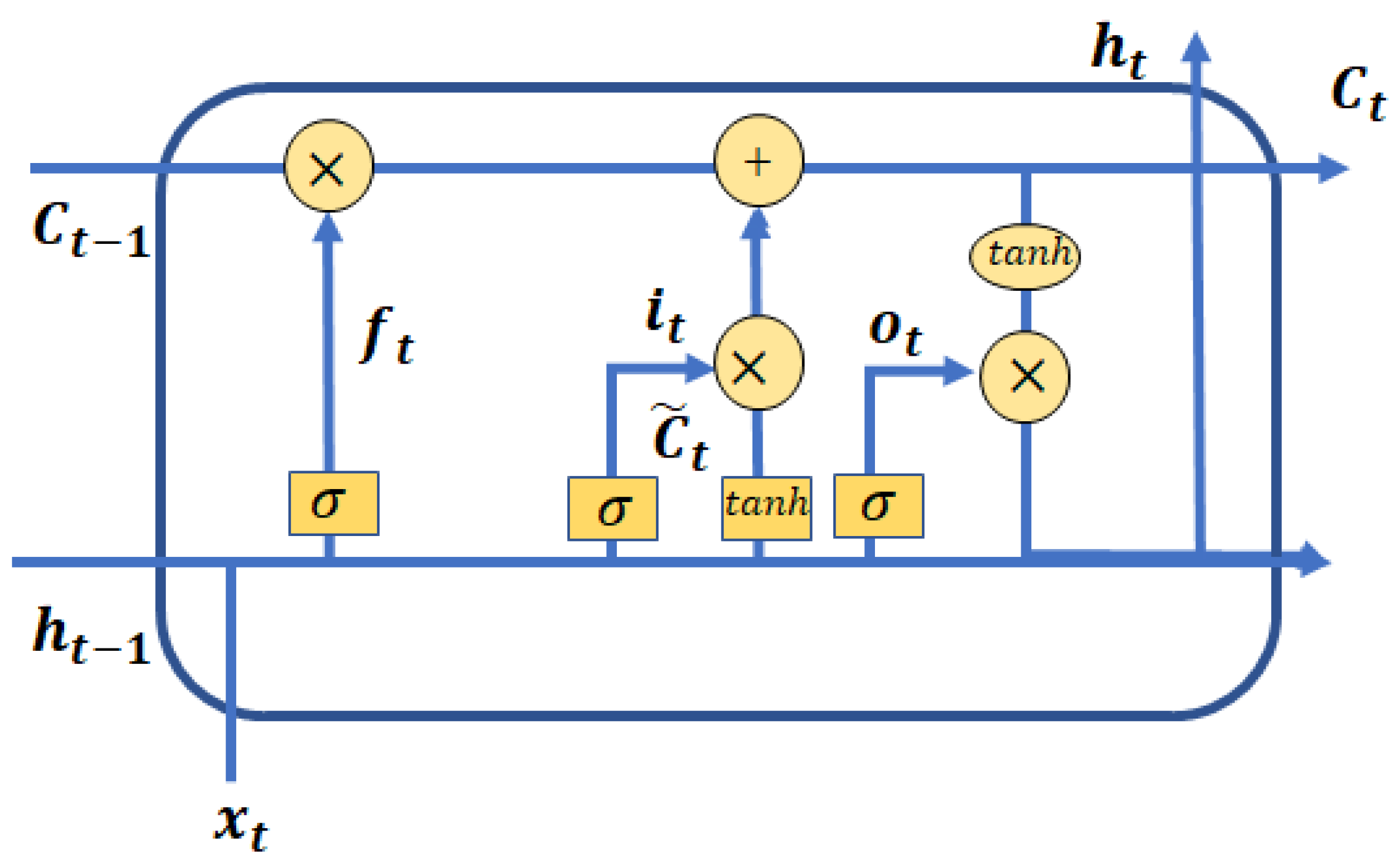
3.2.2. Long Short-Term Memory

Long short-term memory (LSTM) networks are a kind of recurrent neural network (RNN) that is a good candidate for data represented as a sequence, such as time-series and text information (shown in Gers et al. 2000; Hochreiter and Schmidhuber 1997). Learning from large and complex datasets where we can detect the underlying patterns reveals the full potential of LSTM models. Though like most deep learning approaches LSTM-based RNNs have the disadvantage that they are difficult to interpret and to gain an intuition for their behavior, contrary to the AutoRegressive Integrated Moving Average model (ARIMA), LSTM does not rely on assumptions about the data, such as time-series stationarity. The core concept of the LSTM model is the cell state s t that carries relevant information throughout the processing of the sequence, and three different gates that add or remove information from the cell state. At each time step t, the output hidden state h t is updated by the previous hidden state h t 1 and the input through the gate mechanism inside the LSTM layer. There are three gates, each has its purpose:
  • Forget Gate: The forget gate decides what information should be kept or removed from the cell state.
  • Input gate: The input gate decides what information should be added to the cell state.
  • Output gate: The output gate decides what the next hidden state should be.
With the help of the gate functions, we update the cell state and hidden state in each time step. The workflow of LSTM is shown in Figure 2.

3.2.3. GC–LSTM Model

With the two main components (GCN and LSTM) stated above, in this subsection, we describe the workflow of the GC–LSTM algorithm. Instead of simply stacking the GCN unit and LSTM sequentially, the model embeds the GCN unit into the LSTM cell to better integrate structural information. To make the description more clear, the main aforementioned notations are summarized in Table 1 to formulate the dynamic link forecasting problem.
We describe the hidden state updating process carefully with equations step by step below. Firstly, the model decides what information should be kept or removed from the previous cell state performed by the forget gate f t [ 0 , 1 ] . In Equation (2), the graph convolution unit for the forget gate G C N f K utilizing K-hop neighborhood information and current input information A t R N × N is passed through the sigmoid function, which scales the value from zero to one. Zero means that the information is completely forgotten and one means completely remembered.
f t = σ ( A t W z f + G C N f K ( A t 1 , h t 1 ) + b f )
where A t R N × N is the adjacency matrix input at time t and h t 1 R N × d . W z f R N × d and b f R d are the weight and bias term for calculating the forget gate. The next step is to decide what information should be added to the cell state c t [ 1 , 1 ] . Two operations are included in the adding process. The first one is described in Equation (3), the past hidden state h t 1 and current input information A t are passed through the sigmoid function, which scales the value from zero to one. One means the information is important and zero means the information is not important. This is the function for the input gate i t [ 0 , 1 ] . Additionally, the second step is described in Equation (4), which is the candidate’s new value for the cell state. Finally, we use the information of forget gate f t and input gate i t as well as the candidate value c t to update the cell state s t shown in Equation (5). The forget gate information decides the amount of information to be removed from the previous cell state s t 1 and the pointwise multiplication of i t and c t determines what information should to added to the new cell state.
i t = σ ( A t W z i + G C N i K ( A t 1 , h t 1 ) + b i )
c t = t a n h ( A t W z c + G C N c K ( A t 1 , h t 1 ) + b c )
s t = f t G C N s K ( A t 1 , s t 1 ) + i t c t
where W z i , W z c R N × d and b i , b c R d . The function ⊙ represents the Hadamard product. i t , c t and s t are the input gate, new candidates for call state and cell state.
Finally, we calculate the output gate o t and the hidden state h t . Firstly, the graph convolution on past hidden state h t 1 and current input information A t are passed through the sigmoid function. Then, we multiply the t a n h output of the modified cell state with the sigmoid output to decide what information the hidden state should carry.
o t = σ ( A t W z o + G C N o K ( A t 1 , h t 1 ) + b o )
h t = o t t a n h ( s t )

3.2.4. Decoder Model

In order to output the prediction matrix, we adopt a fully connected layer to transform the output hidden state h t to obtain the one-step ahead prediction A t ^ .
A t ^ = σ ( W h h t 1 + b )
where W h R d × N and b R N are the weight and bias term for the fully connected layer. A t ^ [ 0 , 1 ] N × N is the output prediction probability matrix. A higher probability value means that it is more likely to have a relationship at time t.

3.3. Loss Function and Model Training

With the GC–LSTM framework stated above, we need to design a specific loss function and optimizer to train the model. To improve the accuracy of the dynamic link prediction, we would like to design the output probability matrix as close as to the adjacency matrix at time t. A L 2 norm distance could be used in the regression prediction problem by measuring the distance between the prediction probability value and the truth. However, simply using the L 2 distance could not address two problems in the interbank network data. Firstly, as the contagion of systemic risk spreads through existing links, existing links are more important in interbank topology. Secondly, the network snapshots are sparse with a density of less than 10% for daily or weekly activity, which means that there are much more zero elements than nonzero elements. To address the two related problems, the loss function should focus more on the existing links than on nonexisting links in back propagation. Under this assumption, we design a loss function as follows:
L o s s = i N j N ( a i , j , t a i , j , t ^ ) λ i , j
where a i , j , t is the element in adjacency matrix A t and a i , j , t ^ is the element in the output probability matrix A t ^ . For each training process, we give a lower λ i , j value for the existing links and a higher λ i , j value for those nonexisting links. We call Λ = { λ i , j } N × N , i , j = 1 N as the penalty matrix and exert more penalty on nonzero elements. To avoid overfitting, we also employ a regularization term L r e g that is calculated by the sum of squares of the weights in GC–LSTM models. Therefore, the total loss function is defined as:
L o s s t o t a l = L o s s + β L o s s r e g
where β is the trade-off parameter between the two loss functions. To minimize the total loss L o s s t o t a l , we adopt the Adam optimizer in this model.

4. Experiments and Results

In this section, the proposed GC–LSTM model is evaluated on a well-known electronic interbank trading platform called e-MID. We also introduce two baseline models that could be compared with link predictions. Since deep learning types of models are sensitive to parameter tuning, we test the parameter sensitivity and choose the best parameters to train the e-MID dataset. The performance of the link prediction results is evaluated by two metrics AUC and PRAUC.

4.1. e-MID Dataset

The real dataset we adopt is the e-MID interbank market dataset which is the only electronic market for interbank deposits in the Euro area. It was founded in Italy in 1990 and dominated in Euros in 1999. e-MID is the reference marketplace for money market liquidity: according to the “Euro Money Market Study 2006” published by the European Central Bank in February 2007, e-MID accounts for 17% of total turnover in the unsecured money market in the Euro Area (Cassola et al. 2010). Since most of the trading happens in Italy, we chose the top 100 Italian banks from 2005 to 2007 in the e-MID interbank market as our data input. In addition, we want our network density to be reasonably high (greater than 0.05), and we aggregate the daily transaction data into a weekly adjacency matrix. If A i , j , t equals 1, it means that bank i lends to bank j at week t, otherwise there is no trading between them at week t. With the weekly aggregated adjacency matrix as our input, we apply the model to the representative e-MID interbank trading market and understand whether the GC–LSTM model could successfully predict the future interbank trading links compared with the baseline models.
Since most of the trading happens inside Italy, the descriptive statistics are calculated with the top 100 banks trading in Italy. With a weekly aggregated period, we compute various measures of interconnectedness by utilizing the e-MID trading data. Before we introduce the results, we start with the definition of different interconnectedness metrics:
  • Degree: The degree of the network is defined as the number of connections as a proportion of all possible links inside the network (Boss et al. 2004). A low value of the degree might indicate a low level of liquidity in the e-MID interbank market.
  • Clustering coefficient: The clustering coefficient is a measure of how closely nodes in a network cluster together (Soramäki et al. 2007).
  • Centrality: In this part, we introduce three kinds of centrality, which are degree, betweenness, and Eigen centrality. For the degree centrality, it is defined as the number of links incident upon a node (Temizsoy et al. 2017). Since only the node’s immediate ties are considered when calculating degree centrality, it is a local centrality measure. For between centrality, which is introduced by Freeman (1978), it is defined as the number of times a node functions as a bridge along the shortest path between two other nodes, since it focuses on a node’s distance from all other nodes in the network and is a measure of global centrality in this sense. The last centrality measure we introduce is Eigen centrality (Negre et al. 2018). Eigen centrality calculates a node’s centrality based on its neighbors’ centrality, which is a measure of the influence of a node in a network. The score of the Eigen centrality of a bank is between 0 to 1, where higher values indicate more essential banks for interconnection.
  • Largest strongest connected component: A strongly connected component is the portion of a directed graph where each vertex has a route to another vertex. The fraction of banks connected to other banks via directed edges on the network scaled by the total number of banks in the network is defined as the largest strongest connected component of the graph. If the value of the largest strongest connected component is close to 1, it means that the network is highly connected, and if the value is close to zero, the network is much more fragmented.
In Table 2, we show a summary of interconnected statistics for both precrisis and the beginning of the crisis period. With the definition stated above and the null hypothesis that the mean of the underlying statistics between precrisis and crisis is the same, we find that all the statistics in the crisis period are statistically lower than the precrisis period. This means that the crisis diminished the interconnectedness between banks in the e-MID trading networks. Therefore, when we implement the link prediction task, we test both the precrisis period and crisis period and check the performance of both statistical models and the deep learning model in these two periods.

4.2. Baseline Methods

To validate the effectiveness of the proposed GC–LSTM model, we compare it with two baseline models. Other than static network modeling that can be applied to describe relevant characteristics of a network in a variety of ways, there are two streams of dynamic network modeling approaches. Both of them are related to traditional statistical models. The first stream is related to the wide range of latent space models and the second stream is related to the time-series model. For each stream, we choose a typical method as our baseline model. A more detailed introduction of the interbank dynamic link prediction models is described in the Literature Review section. In particular, the two baseline models are introduced as follows:
  • Dynamic latent space model: Dynamic latent space model is a model based on the distance idea in social networks (Hoff et al. 2002). The model assumes that the link probability between any two nodes depends on the distance between the latent position of the two nodes. A dynamic latent space model is proposed by Sewell and Chen (2015) and is used on the interbank network model by Linardi et al. (2020).
  • Discrete autoregressive model: To avoid systemic risk, the information of the counterparty plays an important role to decide who to trade with. The past trading relationship, which is also seen as link persistence, is documented in the paper Papadopoulos and Kleineberg (2019). The relationship is defined as preferential trading and allows banks to ensure liquidity risk in the presence of market frictions such as information and transaction cost (Cocco et al. 2009; Giraitis et al. 2012). Based on the preferential trading theory, the link formation strategy of the Discrete autoregressive model (Jacobs and Lewis 1978) is that the value of a link between bank i and bank j at time t is determined by past value at time t 1 and the ability to create new links. Therefore, the model could be described as follow:
    A i , j , t = θ i . j , t A i , j , t 1 + ( 1 θ i , j , t ) X i , j , t
    where θ i , j , t B ( α i , j ) and X i , j , t B ( χ i , j ) . B ( . ) indicates Bernoulli distribution. The link formation strategy of the Discrete autoregressive model is that the value of a link between bank i and bank j at time t is determined by past value at time t 1 and the ability to create new links.

4.3. Evaluation Metrics

In this study, the performance of the proposed model and compared models are evaluated by commonly used metrics in dynamic link prediction. The Area Under the ROC Curve (AUC) is a commonly used metric to measure the performance of a dynamic link prediction. If the AUC value of the predictor is close to 1, then it is considered more informative. To handle the sparsity problem, the Area Under the Precision-Recall Curve (PRAUC) developed from AUC is designed to deal with the sparsity of networks.

4.4. Parameter Sensitivity
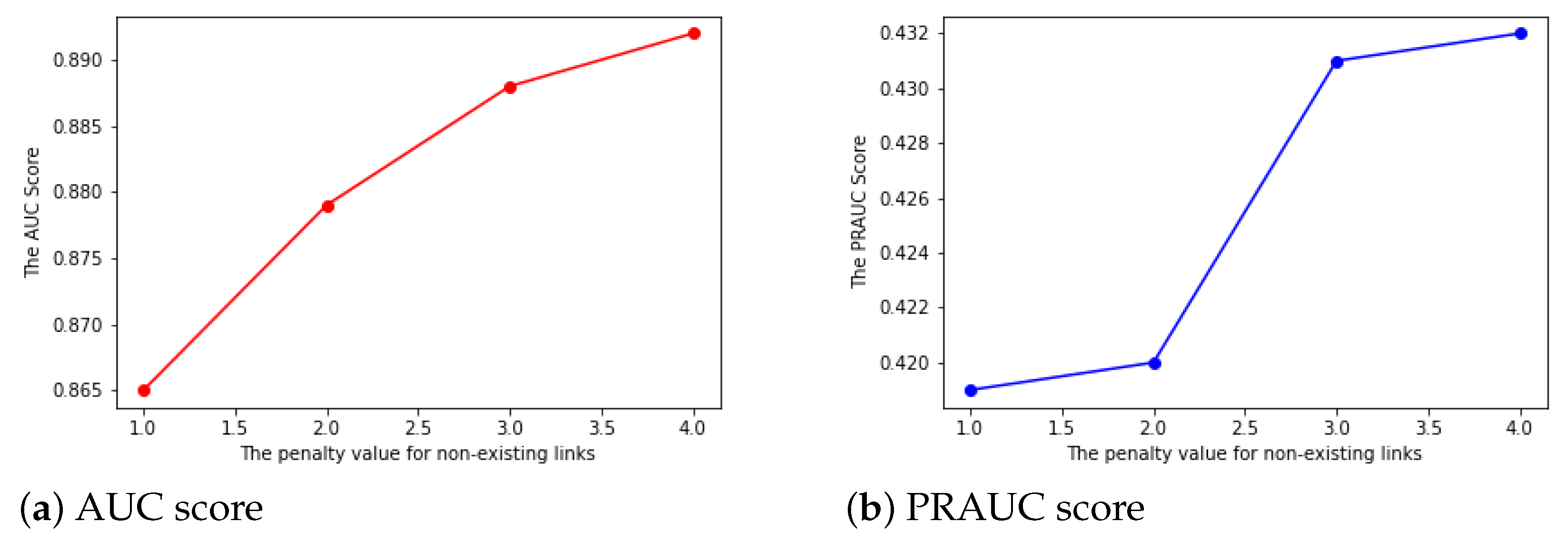
To train the GC–LSTM model, for each epoch, we feed l historical interbank network snapshots ( A t l , , A t 1 ) to predict A t . In the setting, the number of banks (nodes) is N = 100 , and the number of the hidden layer of the GC–LSTM model is d = 12 . The weight decay parameter of the Adam optimizer is 1 × 10 5 and the learning rate is 0.01. Other than parameter settings, the performance of the GC–LSTM model depends on the number of K-hop neighborhoods we used in the GCN unit, the window size l and the penalty λ i , j we use in the loss function:
  • The penalty λ index: As exiting links are much more important than the nonexisting links, we add a penalty to the nonexisting links with a different λ i , j from 1 to 4. Additionally, we set the λ i , j value for the existing links to be 1. If the penalty value is the same for both the existing links and nonexisting links, then we treat the two kinds of links with no difference. The results shown in Figure 3 indicate that a larger penalty could lead to slightly larger AUC and PRAUC. This suggests we choose a higher penalty score for nonexisting links in the following model parameter settings.
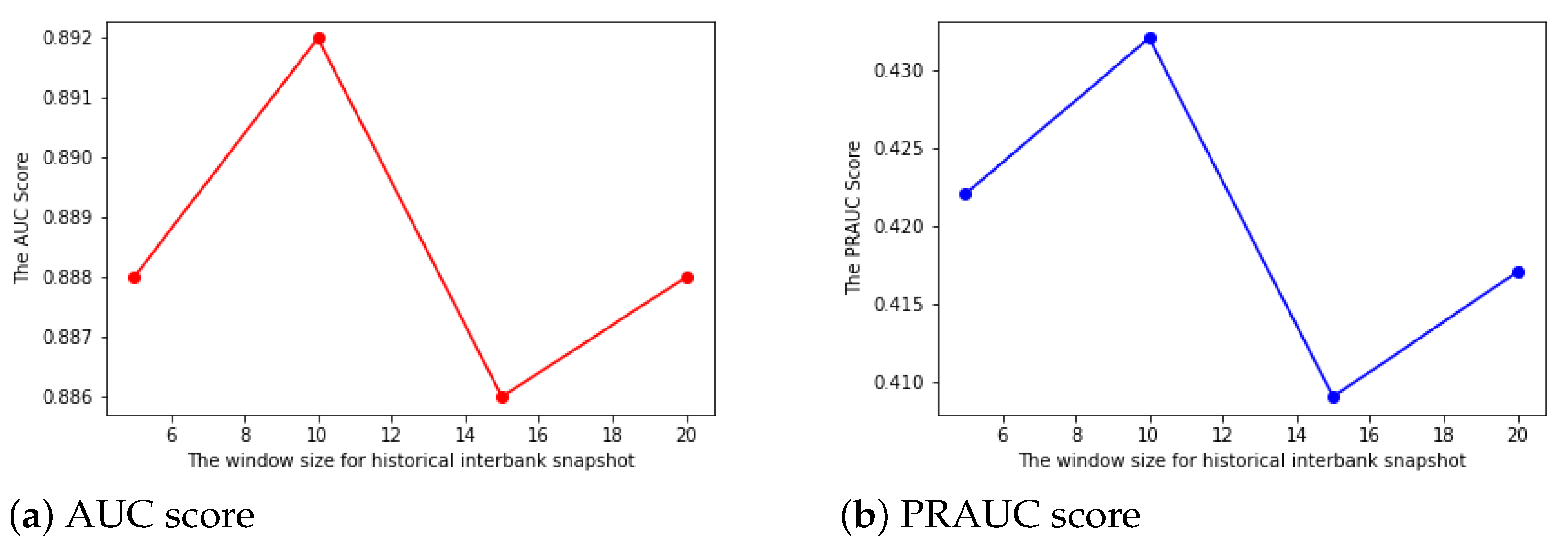
  • The window sizel: In most cases, a larger historical interbank network snapshots input might improve the performance in link prediction. In our case, we use a range of window sizes from 5 to 20 with a regular interval of 5, and the results for both AUC and PRAUC follow a similar pattern. By choosing the window size to be 10, we could achieve both the highest AUC and PRAUC. The results are shown in Figure 4.
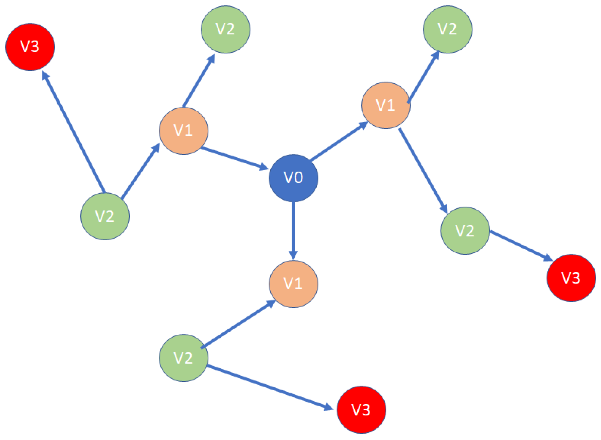
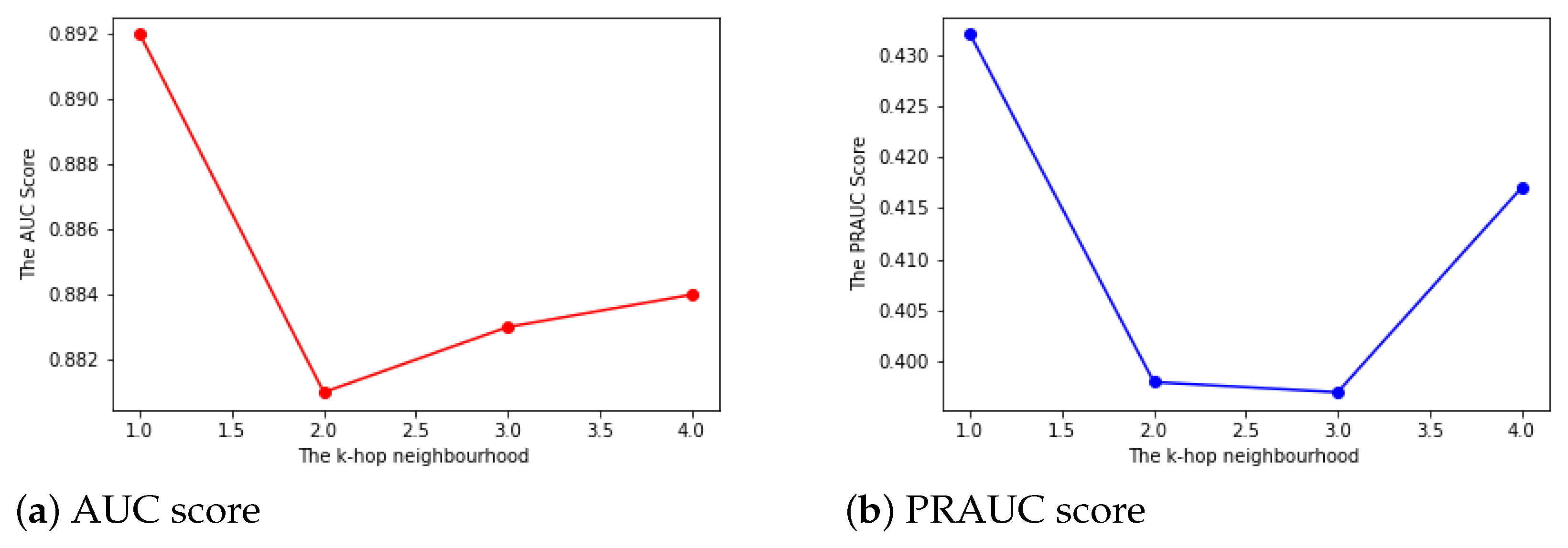
  • TheK-hop neighborhood: The K-hop neighborhood idea comes from social network analysis. The larger the size of K, the more information a node utilizes from its neighborhood. In our interbank network, a larger K does not help in link prediction. It means that if a bank i trades with another bank j, even if bank j has a close relationship to bank z, bank i will not preferentially trade with bank z. The results are shown in Figure 5.

4.5. Link Prediction

With the parameter tuning in the previous section, the model setting is as follows. To train the GC–LSTM model, we feed l historical interbank network snapshots ( A t l , , A t 1 ) to predict A t and use the estimated parameters we obtain from the training process to feed into the network snapshots ( A t , , A t + l 1 ) to obtain the one-step prediction for A t + l . With aggregated weekly data from 2005 to 2007, we have 156 weekly adjacency matrices. Since 2005, we trained and tested the performance on a rolling window basis. In addition, we set l = 10 , and the number of the hidden layers of the GC–LSTM model is d = 12 . The weight decay parameter of the Adam optimizer is 1 × 10 5 and the learning rate is 0.01. We utilize 1-hop neighborhood information, and the penalty value λ is 4. With the model setting stated above, we apply the GC–LSTM model to the top 100 Italian banks and the 36 core European country banks to check the robustness of the model prediction performance. We use the evaluation metrics to check how statistical and deep learning models perform for precrisis and crisis periods. According to Brunetti et al. (2019), the definition of the crisis time starting point is in August 2007. We separate the dataset into two parts and the results are shown in Table 3 and Table 4 for the top 100 Italian banks and Table 5 and Table 6 for core country banks. For both the AUC and PRAUC values, we find that the GC–LSTM model significantly achieves a higher value by using a t-test that measures the difference between the arithmetic means of two samples. The results also indicate that the dynamic latent space model tends to obtain more False positives, and the Discrete autoregressive model tends to obtain more False negatives. The GC–LSTM model is much more balanced than the two baseline models. It achieves a similar False negative but achieves a much lower False positive compared with the Dynamic latent space model. Compared with the Discrete autoregressive model, though it achieves a slightly larger number of False positives, it achieves a smaller number of False negatives and achieves a better AUC and PRAUC. Moreover, we find that, unlike the traditional models that perform worse in the crisis period, the GC–LSTM model performs better in the crisis period, which means that the deep learning model without underlying model assumptions better captures the structure change and achieves better results.

5. Conclusions

In this study, we propose a new deep learning dynamic network link prediction model called GC–LSTM. The entire GC–LSTM model consists of LSTM and GCN, where LSTM is used to learn the temporal characteristics from continuous snapshots, while GCN is used to learn the structural characteristics of the snapshot at each moment. A fully connected layer network is used as a decoder to convert the extracted spatio-temporal features back to the original space that represents the final prediction probability matrix.
To solve the network sparsity problem, we introduce a special loss function with a different penalty for existing and nonexisting links. Finally, we conducted many experiments to compare our GC–LSTM model with the traditional dynamic interbank network model on the e-MID interbank network dataset. The results validate that our model outperforms the others in terms of AUC and PRAUC. Meanwhile, we also compare the results for crisis and precrisis periods for both top 100 Italy banks and core Europe countries’ banks; we find that the deep learning model is better than the traditional model in both crisis time and precrisis periods. In addition, the GC–LSTM model is better at predicting future links in the crisis period than the traditional statistical models, which indicates that the model without statistical underlying assumptions is better at capturing structure change.

Funding

This research received no external funding.

Institutional Review Board Statement

Not applicable.

Informed Consent Statement

Not applicable.

Data Availability Statement

Not applicable.

Conflicts of Interest

The authors declare no conflict of interest.

References

  1. Allen, Franklin, and Douglas Gale. 2000. Financial contagion. Journal of Political Economy 108: 1–33. [Google Scholar] [CrossRef]
  2. Betancourt, Brenda, Abel Rodríguez, and Naomi Boyd. 2017. Bayesian fused lasso regression for dynamic binary networks. Journal of Computational and Graphical Statistics 26: 840–50. [Google Scholar] [CrossRef]
  3. Boss, Michael, Helmut Elsinger, Martin Summer, and Stefan Thurner 4. 2004. Network topology of the interbank market. Quantitative Finance 4: 677–84. [Google Scholar] [CrossRef]
  4. Bräuning, Falk, and Falko Fecht. 2012. Relationship Lending and Peer Monitoring: Evidence from Interbank Payment Data. Working Paper. Available online: https://papers.ssrn.com/sol3/papers.cfm?abstract_id=2020171 (accessed on 13 March 2012).
  5. Bräuning, Falk, and Siem Jan Koopman. 2020. The dynamic factor network model with an application to international trade. Journal of Econometrics 216: 494–515. [Google Scholar] [CrossRef]
  6. Brunetti, Celso, Jeffrey H. Harris, Shawn Mankad, and George Michailidis. 2019. Interconnectedness in the interbank market. Journal of Financial Economics 133: 520–38. [Google Scholar] [CrossRef] [Green Version]
  7. Cassola, Nuno, Cornelia Holthausen, and Marco Lo Duca. 2010. The 2007/2009 turmoil: A challenge for the integration of the euro area money market. Paper presented at ECB Workshop on Challenges to Monetary Policy Implementation beyond the Financial Market Turbulence, Frankfurt am Main, Germany, November 30–December 1. [Google Scholar]
  8. Chen, Jinyin, Xueke Wang, and Xuanheng Xu. 2021. Gc-lstm: Graph convolution embedded lstm for dynamic network link prediction. Applied Intelligence 52: 7513–28. [Google Scholar] [CrossRef]
  9. Cocco, Joao F., Francisco J. Gomes, and Nuno C. Martins. 2009. Lending relationships in the interbank market. Journal of Financial Intermediation 18: 24–48. [Google Scholar] [CrossRef]
  10. Denbee, Edward, Christian Julliard, Ye Li, and Kathy Yuan. 2021. Network risk and key players: A structural analysis of interbank liquidity. Journal of Financial Economics 141: 831–59. [Google Scholar] [CrossRef]
  11. Durante, Daniele, and David B. Dunson. 2016. Locally adaptive dynamic networks. The Annals of Applied Statistics 10: 2203–32. [Google Scholar] [CrossRef]
  12. Elliott, Matthew, Benjamin Golub, and Matthew O. Jackson. 2014. Financial networks and contagion. American Economic Review 104: 3115–53. [Google Scholar] [CrossRef] [Green Version]
  13. Freeman, Linton C. 1978. Centrality in social networks conceptual clarification. Social Networks 1: 215–39. [Google Scholar] [CrossRef] [Green Version]
  14. Freixas, Xavier, Bruno M. Parigi, and Jean-Charles Rochet. 2000. Systemic risk, interbank relations, and liquidity provision by the central bank. Journal of Money, Credit and Banking 32: 611–38. [Google Scholar] [CrossRef] [Green Version]
  15. Gai, Prasanna, Andrew Haldane, and Sujit Kapadia. 2011. Complexity, concentration and contagion. Journal of Monetary Economics 58: 453–70. [Google Scholar] [CrossRef]
  16. Gai, Prasanna, and Sujit Kapadia. 2010. Contagion in financial networks. Proceedings of the Royal Society A: Mathematical, Physical and Engineering Sciences 466: 2401–23. [Google Scholar] [CrossRef] [Green Version]
  17. Gers, Felix A., Jürgen Schmidhuber, and Fred Cummins. 2000. Learning to forget: Continual prediction with lstm. Neural Computation 12: 2451–71. [Google Scholar] [CrossRef]
  18. Giraitis, Liudas, George Kapetanios, Anne Wetherilt, and Filip Žikeš. 2012. Estimating the dynamics and persistence of financial networks, with an application to the sterling money market. Journal of Applied Econometrics 31: 58–84. [Google Scholar] [CrossRef]
  19. Hatzopoulos, Vasilis, Giulia Iori, Rosario N. Mantegna, Salvatore Micciche, and Michele Tumminello. 2015. Quantifying preferential trading in the e-mid interbank market. Quantitative Finance 15: 693–710. [Google Scholar] [CrossRef]
  20. Hochreiter, Sepp, and Jürgen Schmidhuber. 1997. Long short-term memory. Neural Computation 9: 1735–80. [Google Scholar] [CrossRef]
  21. Hoff, Peter D., Adrian E. Raftery, and Mark S. Handcock. 2002. Latent space approaches to social network analysis. Journal of the American Statistical Association 97: 1090–98. [Google Scholar] [CrossRef]
  22. Jacobs, Patricia A., and Peter A. W. Lewis. 1978. Discrete time series generated by mixtures. I: Correlational and runs properties. Journal of the Royal Statistical Society: Series B (Methodological) 40: 94–105. [Google Scholar] [CrossRef]
  23. Kipf, Thomas N., and Max Welling. 2017. Semi-supervised classification with graph convolutional networks. arXiv arXiv:1609.02907. [Google Scholar]
  24. Leventides, John, Kalliopi Loukaki, and Vassilios G. Papavassiliou. 2019. Simulating financial contagion dynamics in random interbank networks. Journal of Economic Behavior & Organization 158: 500–25. [Google Scholar]
  25. Linardi, Fernando, Cees Diks, Marco van der Leij, and Iuri Lazier. 2020. Dynamic interbank network analysis using latent space models. Journal of Economic Dynamics and Control 112: 103792. [Google Scholar] [CrossRef] [Green Version]
  26. Mazzarisi, Piero, Paolo Barucca, Fabrizio Lillo, and Daniele Tantari. 2019. A dynamic network model with persistent links and node-specific latent variables, with an application to the interbank market. European Journal of Operational Research 281: 50–65. [Google Scholar] [CrossRef] [Green Version]
  27. Negre, Christian F. A., Uriel N. Morzan, Heidi P. Hendrickson, Rhitankar Pal, George P. Lisi, J. Patrick Loria, Ivan Rivalta, Junming Ho, and Victor S. Batista. 2018. Eigenvector centrality for characterization of protein allosteric pathways. Proceedings of the National Academy of Sciences USA 115: E12201–E12208. [Google Scholar] [CrossRef] [Green Version]
  28. Nier, Erlend, Jing Yang, Tanju Yorulmazer, and Amadeo Alentorn. 2007. Network models and financial stability. Journal of Economic Dynamics and Control 31: 2033–60. [Google Scholar] [CrossRef]
  29. Papadopoulos, Fragkiskos, and Kaj-Kolja Kleineberg. 2019. Link persistence and conditional distances in multiplex networks. Physical Review 99: 012322. [Google Scholar] [CrossRef] [Green Version]
  30. Polson, Nicholas G., James G. Scott, and Jesse Windle. 2013. Bayesian inference for logistic models using pólya–gamma latent variables. Journal of the American statistical Association 108: 1339–49. [Google Scholar] [CrossRef] [Green Version]
  31. Sarkar, Purnamrita, and Andrew Moore. 2005. Dynamic social network analysis using latent space models. Advances in Neural Information Processing Systems 18: 1145. [Google Scholar] [CrossRef]
  32. Sarkar, Purnamrita, Deepayan Chakrabarti, and Michael Jordan. 2012. Nonparametric link prediction in dynamic networks. arXiv arXiv:1206.6394. [Google Scholar]
  33. Sewell, Daniel K., and Yuguo Chen. 2015. Latent space models for dynamic networks. Journal of the American Statistical Association 110: 1646–57. [Google Scholar] [CrossRef]
  34. Soramäki, Kimmo, Morten L. Bech, Jeffrey Arnold, Robert J. Glass, and Walter E. Beyeler. 2007. The topology of interbank payment flows. Physica A: Statistical Mechanics and Its Applications 379: 317–33. [Google Scholar] [CrossRef] [Green Version]
  35. Temizsoy, Asena, Giulia Iori, and Gabriel Montes-Rojas. 2017. Network centrality and funding rates in the e-mid interbank market. Journal of Financial Stability 33: 346–65. [Google Scholar] [CrossRef]
  36. Upper, Christian. 2011. Simulation methods to assess the danger of contagion in interbank markets. Journal of Financial Stability 7: 111–25. [Google Scholar] [CrossRef]
  37. Zhou, Shuheng, John Lafferty, and Larry Wasserman. 2010. Time varying undirected graphs. Machine Learning 80: 295–319. [Google Scholar] [CrossRef] [Green Version]
Figure 1. K-hop neighborhood. The blue node is the source node, the area that covers the yellow nodes is the 1-hop neighborhood, the area that covers the yellow and green nodes are the 2-hop neighbors, and the area that covers the yellow, green and red nodes is the 3-hop neighborhood.
Ijfs 10 00054 g001
Figure 2. Architecture of Long short-term memory model. The notations of the graph are shown as follows. f t , i t , o t are the forget gate, input gate and output gate. C t is the cell state, C ˜ t is the new candidate values, x t is the input at time t and h t is the hidden state. × is the pointwise multiplication operation, + is the addition operation, σ is the sigmoid function and t a n h is the hyperbolic tangent function.
Ijfs 10 00054 g002
Figure 3. The evaluation metrics with different penalty scores. In (a,b), we use the window size l = 10 and 1-hop neighborhood GCN units. We set the penalty from 1 to 4, and the performance of AUC and PRAUC scores are shown in (a,b).
Ijfs 10 00054 g003
Figure 4. The evaluation metrics with different historical time periods. In (a,b), we use the penalty value equal to 4 and 1-hop neighborhood GCN units. We set the window size from 5 to 20, and the performance of AUC and PRAUC scores are shown in (a,b).
Ijfs 10 00054 g004
Figure 5. The evaluation metrics with different K values. In (a,b), we use the window size l = 10 and the penalty value for nonexisting links are 4. We set the K-hop neighborhood for the GCN units from 1 to 4, and the performance of AUC and PRAUC scores are shown in (a,b).
Ijfs 10 00054 g005
Table 1. Notations used in the GC–LSTM framework.
NotationDescription
A t the adjacency matrix of the interbank network snapshot at time t
lthe window size for prediction
Nthe number of banks (nodes) in the network
dthe number of hidden layers in the GC–LSTM model
T k Chebyshev polynomial function
A t ^ the output probability matrix at time t
b f , b c , b i , b o the bias terms in gate function
W z f , W z c , W z i , W z o the weight terms in gate function
G C N K the graph convolutional operation
λ i , j penalty parameter in Equation (9)
Table 2. Summary statistics of weekly aggregated e-MID interbank network in top 100 Italian banks. The average degree in each network is referred to as Degree. The clustering coefficient is denoted as the Clustering coefficient. The three different centrality measures are degree centrality, betweenness centrality and Eigen centrality. Additionally, the fraction of nodes in the largest strongly connected component is the largest strongest connected component. The significance levels of 10% (*), 5% (**) and 1% (***) are used to assess the mean difference between the crisis and the precrisis period with the t-test.
Time PeriodInterconnectedness StatisticsMeanStandard Deviation
All data resultsDegree0.06700.0090
Clustering coefficient0.11570.0296
Betweenness centrality0.00450.0024
Eigen centrality0.05060.0039
Degree centrality0.13400.0180
Largest strongest connected component0.18920.1241
PrecrisisDegree0.06820.0081
Clustering coefficient0.12070.0269
Betweenness centrality0.00480.0023
Eigen centrality0.05080.039
Degree centrality0.13650.0162
Largest strongest connected component0.20060.1229
CrisisDegree 0.0621 ***0.0058
Clustering coefficient 0.0888 ***0.0248
Betweenness centrality 0.0025 ***0.0015
Eigen centrality 0.0491 *0.0036
Degree centrality 0.1242 ***0.0115
Largest strongest connected component 0.1267 **0.1085
Table 3. AUC score for three models in the top 100 Italian banks. The significance level of 1% (***) is used to assess the mean difference between the benchmark models (DAR or Latent space model) and the GC–LSTM model with the t-test.
Time PeriodMethodsMean AUCStandard Deviation
All data resultsDAR 0.695 ***0.036
Latent Space Model 0.777 ***0.023
GC–LSTM0.8950.016
PrecrisisDAR 0.703 ***0.034
Latent Space Model 0.784 ***0.018
GC–LSTM0.8930.016
CrisisDAR 0.660 ***0.018
Latent Space Model 0.746 ***0.019
GC–LSTM0.9050.013
Table 4. PRAUC score for three models in the top 100 Italian banks. The significance level of 1% (***) is used to assess the mean difference between the benchmark models (DAR or Latent space model) and the GC–LSTM model with the t-test.
Time PeriodMethodsMean PRAUCStandard Deviation
All data resultsDAR 0.390 ***0.054
Latent Space Model 0.152 ***0.021
GC–LSTM0.4310.038
PrecrisisDAR 0.401 ***0.049
Latent Space Model 0.158 ***0.017
GC–LSTM0.4320.038
CrisisDAR 0.349 ***0.032
Latent Space Model 0.125 ***0.017
GC–LSTM0.4260.035
Table 5. AUC score for three models in the core country banks. The significance level of 1% (***) is used to assess the mean difference between the benchmark models (DAR or Latent space model) and the GC–LSTM model with the t-test.
Time PeriodMethodsMean AUCStandard Deviation
All data resultsDAR 0.666 ***0.051
Latent Space Model 0.717 ***0.095
GC–LSTM0.7820.054
PrecrisisDAR 0.670 ***0.048
Latent Space Model 0.709 ***0.039
GC–LSTM0.7790.056
CrisisDAR 0.650 ***0.057
Latent Space Model 0.753 ***0.025
GC–LSTM0.7950.042
Table 6. PRAUC score for three models in the core country banks. The significance level of 1% (***) is used to assess the mean difference between the crisis and the precrisis period with the t-test.
Time PeriodMethodsMean PRAUCStandard Deviation
All data resultsDAR 0.175 ***0.040
Latent Space Model 0.094 ***0.023
GC–LSTM0.2750.074
PrecrisisDAR 0.177 ***0.042
Latent Space Model 0.092 ***0.024
GC–LSTM0.4320.075
CrisisDAR 0.170 ***0.030
Latent Space Model 0.105 ***0.013
GC–LSTM0.4260.065
Publisher’s Note: MDPI stays neutral with regard to jurisdictional claims in published maps and institutional affiliations.

