Dynamic Factor Rotation Strategy: A Business Cycle Approach

Abstract

This study developed an investment framework to implement dynamic factor rotation strategies according to changes in economic conditions. I constructed a useful macro indicator that tracked real-time business cycles of the US economy and applied a trend-filtering method to the indicator to identify economic regimes based on the level and momentum change. I found that historical performance of individual equity factors greatly differed across economic regimes, and this heterogeneity can be exploited to build dynamic factor rotation strategies by shifting exposures toward effective factors according to the different regimes. The out-of-sample analysis showed that the regime-based dynamic approach outperformed the static benchmark in terms of absolute and risk-adjusted returns after accounting for transaction costs. The results have important implications for many pension funds and for institutional investors interested in factor investing and seeking to improve the long-term portfolio performance.

1. Introduction

Factor investing has gained great attention in many pension funds and institutional investors since the 2007–2008 Global Financial Crisis (GFC). It is an investment approach that involves providing systematic exposures to risk factors in order to enhance diversification and generate above-market returns. Although the benefits of factor investing have been widely documented in the literature, including Clarke et al. (2005), Bass et al. (2017), Dimson et al. (2017), and Bergeron et al. (2018), optimal management of factor allocations still remains controversial. In particular, whether a forecasting-based dynamic factor allocation can add greater value than a static factor allocation is still the subject of debate, given the diversification benefits of factor allocations.

This study investigated how to allocate individual equity factors dynamically, which is generally referred to as “factor timing”. Specifically, this study aimed to provide a dynamic factor rotation strategy based on changes in economic regimes and to examine the profitability of the dynamic strategy. The regime-based dynamic factor approach was motivated by extensive previous studies, such as Harvey (1989), Ferson and Harvey (1991), Ilmanen et al. (2014), Hodges et al. (2017), and Amenc et al. (2019), highlighting that factor premiums are highly cyclical and closely linked to macroeconomic conditions. For example, size factor tends to perform well when the economy recovers from a trough, while momentum factor tends to outperform when the economy expands and trends become well-established.

My factor-tilting strategy began by assessing the prevailing economic regime to determine which factors were likely to outperform in the environment. To do so, similar to Vliet and Blitz (2011) and Blin et al. (2021), this study developed a useful macro indicator that tracked real-time business cycles of the US economy and adopted a nowcasting approach to implement dynamic factor rotation strategies. In particular, this study presented a practical and novel methodology to characterize economic regimes. Specifically, the l₁ trend-filtering method suggested by Kim et al. (2009) was applied to the macro indicator, and economic regimes were identified based on the level and momentum change. The selection of the l₁ trend filtering was motivated by its popularity in various fields, including economics and finance when detecting momentum changes. I then demonstrated that individual factor performance varies markedly across economic cycles, and this heterogeneity can be exploited to build dynamic factor rotation strategies by tilting exposures toward effective factors according to the different regimes.

This study conducted an out-of-sample performance analysis to examine the profitability of the regime-based dynamic strategy. A risk parity portfolio, which has been broadly used in the asset management industry, was constructed as a benchmark for performance comparison. To build the dynamic factor portfolio, I adopted the methodology proposed by Haesen et al. (2017) and Jurczenko and Teiletche (2018) of using the Black–Litterman approach by embedding a regime-based active view on expected factor returns into the benchmark. The choice of the methodology for the dynamic factor portfolio was based on the popularity of the Black–Litterman approach when implementing a dynamic strategy in portfolio management. The out-of-sample results indicate that the regime-based dynamic approach produced a significant increase in absolute and risk-adjusted returns, even if it increased the overall volatility and average turnover. Most importantly, after taking transaction costs into account, the active strategy still remained statistically and economically significant.

My research is intimately related to the ongoing debate about the potential benefits of factor timing relative to a diversified passive factor allocation. Most of the studies have been split between skeptics and optimists up to this day. The skeptics, such as Asness (2016), Asness et al. (2017), Lee (2017), and Dichtl et al. (2019), claim that factor timing is not significantly beneficial because of high transaction costs and because factor diversification easily outperforms the potential of factor timing. On the other hand, the optimists, such as Hodges et al. (2017), Bender et al. (2018), Polk et al. (2020), Scherer and Apel (2020), and Blin et al. (2021), argue that factor timing based on market, sentiment, and macroeconomic indicators is still economically meaningful.

This study contributed to the literature supporting the potential benefits of factor timing in several ways. First, this study created a real-time macro indicator for the US economy and showed its effectiveness of detecting economic regimes and executing regime-based dynamic strategies. Second, in contrast with previous studies including Hodges et al. (2017) and Blin et al. (2021) that relied on ad hoc classifications of macroeconomic environments, this study provided a practical and transparent methodology to characterize economic regimes by applying a trend-filtering method to the indicator. This model-free approach has a large advantage over the commonly used Markov-switching model, which involves high uncertainty of parameter estimation and high sensitivity to out-of-sample analysis. Finally, compared to extant studies, this study conducted a rigorous out-of-sample analysis using longer historical data and testing periods to prove the profitability of regime-based dynamic factor rotation strategies.

The remainder of this paper proceeds as follows. Section 2 describes how to construct the macro indicator, and Section 3 presents the methodology of defining economic regimes. Section 4 discusses factor-return characteristics across economic regimes, and Section 5 explains how to construct factor portfolios. Section 6 reports the main empirical results, and Section 7 checks the robustness of the results. Section 8 concludes the paper.

2. Macro Indicator

This section describes how to construct a monthly macro indicator that tracks real-time business cycles of the US economy. One can think of the macro indicator as a nowcasting indicator that has been broadly adopted in applied macroeconomic work due to its effectiveness for assessing economic conditions, as argued by Beber et al. (2015) and Bok et al. (2017).

Providing economic information in a timely manner is critical when connecting macro conditions with asset returns because financial markets tend to lead real economic activity. In this regard, the macro indicator consisted of the following five leading variables: Yield spread between the 10-year treasury yield and effective federal fund rate, credit spread between the Moody’s Baa corporate bond yield and 10-year treasury yield, four-week moving average of initial jobless claims, total units of building permits, and CBOE Volatility Index (VIX). The selection of the indicators was based on the well-established empirical and theoretical evidence. For example, from the empirical side, Ang et al. (2006) and Gilchrist et al. (2009) highlighted the importance of the yield spread and credit spread in predicting US economic slowdowns, respectively. Liu and Moench (2016) also empirically supported the role of the variables mentioned above in predicting US recessions. From the theoretical side, Bloom (2009) built a structural model to show that uncertainty measured by the VIX index is an important source of macroeconomic fluctuations, with an increased uncertainty reducing consumption and investment significantly. All data are easily available at the Federal Reserve Economic Data maintained by the St. Louis Federal Reserve Bank and cover the sample period from January 1967 to October 2021.1

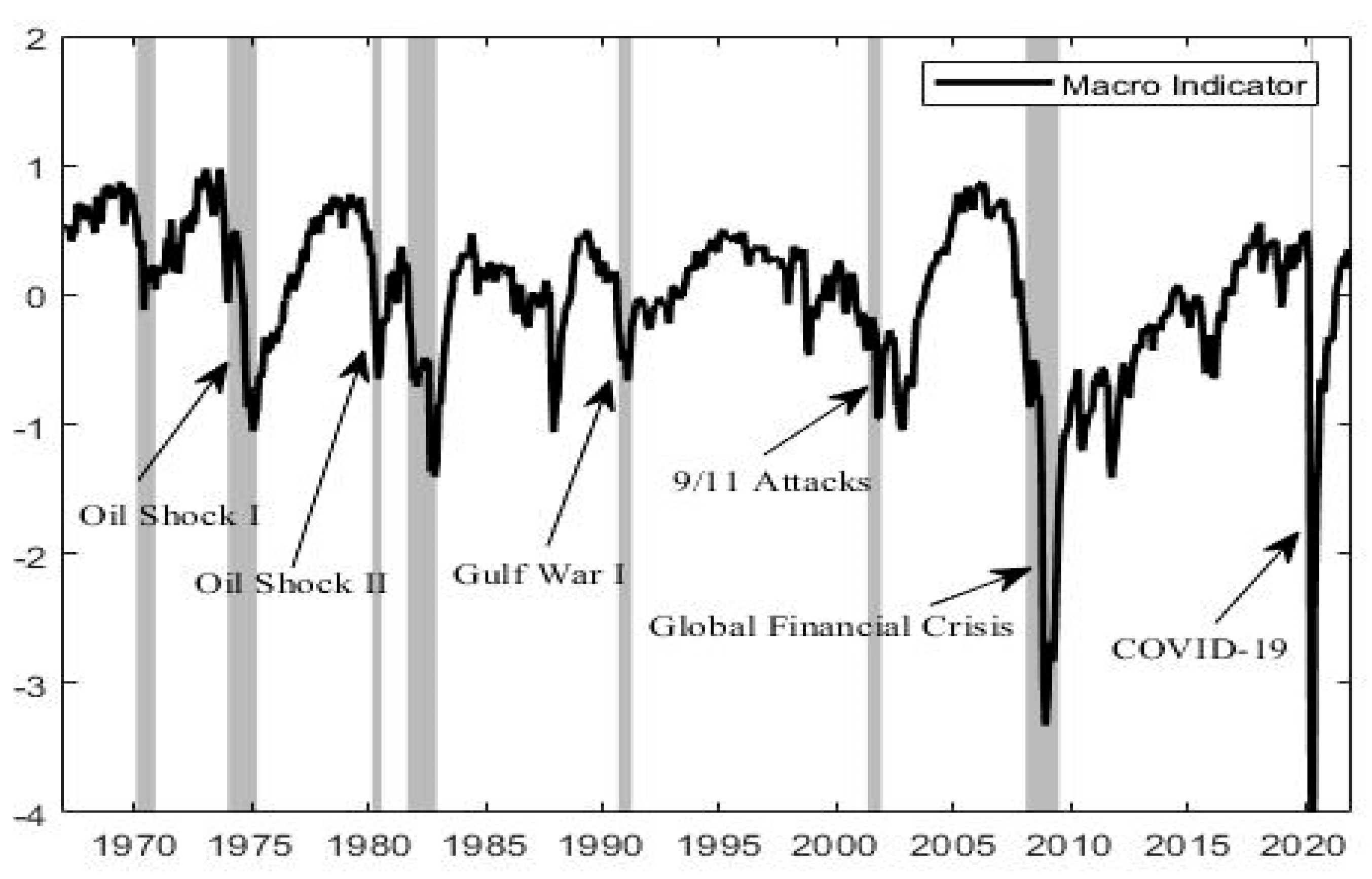
Each variable was normalized to have zero mean and unit standard deviation.2 Applying principal components analysis, I extracted the first principal component of the five normalized variables and used it as the macro indicator. Figure 1 shows its historical trend with the National Bureau of Economic Research (NBER) recession periods denoted by shaded areas. Every economic cycle tended to exhibit recurring patterns over time with expansions followed by contractions, even though it differed in duration and persistence. In particular, a peak-to-trough decline in the macro indicator was broadly consistent with almost all NBER recession periods, including the two severe recessions of the 2007–2008 GFC and the recent COVID-19 pandemic.

3. Economic Regimes

There are many different ways to model and identify economic regimes. Markov-switching modelling is one of the most commonly used methods (e.g., Hamilton 1989; Chauvet 1998; Song 2014). However, the major problem with the Markov-switching model is the high sensitivity of parameter estimation and regime changes with respect to out-of-sample analysis. In recent years, several study, such as those done by Vliet and Blitz (2011), Ilmanen et al. (2014), Jurczenko and Teiletche (2018), and Blin et al. (2021), have relied on direct identification of economic regimes based on simple transformations of various macroeconomic and financial indicators. This study also took a similar approach to identify real-time economic regimes in a purely data-driven manner. Specifically, using the macro indicator, I classified the different stages of the business cycle based on the level and momentum change in economic activity and defined the following four economic regimes:

• Recovery: Economic activity below average level and accelerating.
• Expansion: Economic activity above average level and accelerating.
• Slowdown: Economic activity above average level and decelerating.
• Contraction: Economic activity below average level and decelerating.

Since the macro indicator is already standardized, one can easily discern the level of economic activity based on its sign. That is, if it is positive, then the level of economic activity is above average, and if it is negative, then the level of economic activity is below average. To extract the momentum change in economic activity, I applied a trend-filtering algorithm to the macro indicator and obtained a trend function by filtering out noise. More precisely, similar to Mulvey and Liu (2016), the l₁ trend-filtering method developed by Kim et al. (2009), which is commonly adopted in various fields including economics and finance, was used to detect the momentum change. The l₁ trend filter solved the following objective function to acquire the trend estimate (x_t):

$$\min \left(\frac{1}{2}\right){\displaystyle \sum }_{t=0}^n{\left(y_t-x_t\right)}^2+\lambda {\displaystyle \sum }_{t=0}^{n-1}\left|x_{t-1}-2x_t+x_{t+1}\right|,$$

where y_t is the original time series data, i.e., the macro indicator in this study, and $\lambda \ge 0$ is a regularization parameter that controls the trade-off between the size of the residual (y_t − x_t) and smoothness of the estimated trend.3 The l₁ trend-filtering method leads to a piecewise linear trend estimate, i.e., an affine function over each time interval, and the kink points represent the change in the slope of the estimated trend, which can be interpreted as the momentum change in economic activity. If the slope of the estimated trend is positive, economic activity is considered to accelerate, and if it is negative, economic activity is considered to decelerate.

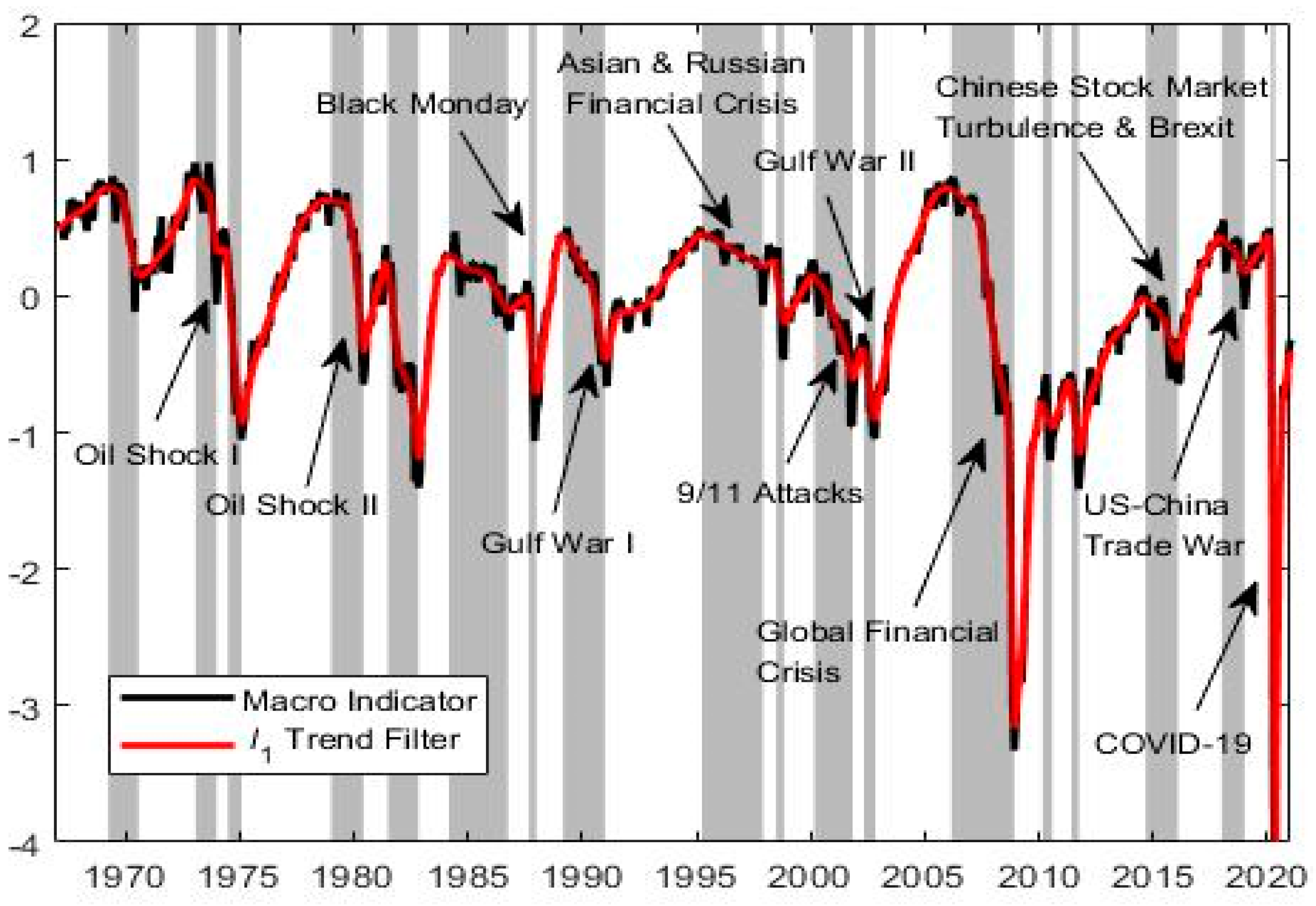
Figure 2 illustrates a regime plot of the macro indicator for the past 50 years. Gray areas refer to regimes in which momentum in economic activity was decelerating, whereas light areas represent regimes in which it was accelerating. The momentum-decelerating regimes contain not only the NBER recession periods but also several global events, including the 1997 Asian financial crisis, 2015 Chinese stock market turbulence, and 2018 US–China trade war. Having characterized economic regimes, I computed their transition matrix and distribution.

Table 1. Transition matrix and distribution of economic regimes.

Transition Matrix					Total #
From/To	Recovery	Expansion	Slowdown	Contraction
Recovery	94%	5%	0%	1%	172
Expansion	0%	93%	7%	0%	215
Slowdown	0%	3%	92%	5%	168
Contraction	10%	0%	0%	90%	102

presents the results. Each regime tended to stay at its current state over time with the probability ranging from 90% to 94%. In particular, the duration of slowdown and contraction regimes was much shorter than that of recovery and expansion regimes. These findings are in line with the well-documented features of the US business cycle. That is, economic conditions tended to improve gradually, followed by a short and dramatic decline.

4. Factor-Return Characteristics

This section discusses which factors were used for dynamic factor allocations and describes their historical characteristics across macroeconomic regimes. I focused on five equity factors that are widely adopted and well-documented in academic research: size, value, momentum, profitability, and investment.4 Starting with the influential studies of Fama and French (1992) and Fama and French (1993), a considerable body of literature, including Carhart (1997); Novy-Marx (2013); Fama and French (2015); and Fama and French (2016), proves that each factor has delivered positive long-term premiums and possesses significant information in explaining the cross-section of average stock returns. All factor data are monthly and can be easily obtained from the Kenneth French’s data library, covering the period from January 1967 to October 2021.

Table 2. Historical characteristics of factor returns for January 1967–October 2021.

	Size	Value	Momentum	Profitability	Investment
Panel A: Descriptive Statistics
Annualized return (%)	2.622	3.165	7.312	3.328	3.311
Annualized volatility (%)	10.627	10.273	14.879	7.751	6.906
Sharpe ratio	0.247	0.308	0.491	0.429	0.479
Skewness	0.371	0.016	−1.273	−0.358	0.369
Excess kurtosis	0.182	−1.157	6.627	8.987	−1.790
Panel B: Correlation Matrix
Size	1.000	−0.019	−0.088	−0.364	−0.076
Value	−0.019	1.000	−0.220	0.105	0.673
Momentum	−0.088	−0.220	1.000	0.089	−0.018
Profitability	−0.364	0.105	0.089	1.000	−0.015
Investment	−0.076	0.673	−0.018	−0.015	1.000
Panel C: Diversification Metrics
Average correlation	−0.137	0.135	−0.059	−0.046	0.141

demonstrates descriptive statistics for individual equity factors over the full sample periods. Panel A shows that most of the factors posted similar annualized returns of around 2–3%, with the noticeable exception of the momentum factor, which had the highest annualized return of 7.3%. Although momentum was the best-performing factor, it had the highest volatility of 14.9%, which was twice as much as the volatility of investment factor. In terms of the risk-adjusted return, the momentum factor was the highest, largely due to the high absolute return, followed by the investment factor, mainly due to the low volatility. As evidenced by the skewness and excess kurtosis, the return distribution of each factor differed markedly in the degree of asymmetry and tailedness. For instance, the momentum and profitability factors had a highly fat-tailed return distribution, with relatively high probability of obtaining extreme outcomes. In particular, the momentum factor had the highest tail risk as evidenced by strong negative skewness. As reported in Panel B, most of the factors were not extremely correlated, ranging from −0.364 to 0.105, suggesting the diversification potential of factor combinations. One exception was the value and investment factors, both of which had a strong positive correlation of 0.673. As mentioned by Fama and French (2015), this positive relation was largely due to the fact that high-value firms tend to be low-investment firms. As described in Panel C, size factor had the lowest average correlation, indicating that its poor performance in absolute and risk-adjusted returns was somewhat compensated by its diversifying property.

Table 3. Factor-return characteristics across economic regimes.

	Size	Value	Momentum	Profitability	Investment
Panel A: Recovery
Annualized return (%)	10.319	0.977	−3.616	0.210	1.808
Annualized volatility (%)	9.241	9.954	17.096	7.515	6.589
Sharpe ratio	1.117	0.098	−0.212	0.028	0.274
Panel B: Expansion
Annualized return (%)	6.143	4.299	14.744	0.974	1.555
Annualized volatility (%)	9.512	9.119	10.854	6.005	6.240
Sharpe ratio	0.645	0.471	1.358	0.162	0.249
Panel C: Slowdown
Annualized return (%)	−5.612	2.457	7.128	3.933	3.128
Annualized volatility (%)	11.666	9.328	13.283	8.368	6.241
Sharpe ratio	−0.481	0.263	0.537	0.470	0.501
Panel D: Contraction
Annualized return (%)	−4.018	5.357	13.946	11.461	9.503
Annualized volatility (%)	11.588	13.689	18.608	9.429	8.966
Sharpe ratio	−0.347	0.391	0.749	1.216	1.060

shows the historical performance of individual equity factors across the different stages of the business cycle. Overall, factor performance seemed to be intimately linked to macro environments and to have strong cyclicality. Specifically, size factor tended to perform well during recovery regimes, as evidenced by a high Sharpe ratio of 1.117, whereas momentum factor exhibited poor performance. During expansion regimes when both the economy and stock prices had well-established trends, momentum factor tended to outperform significantly, and its performance declined during slowdown regimes, even though the relative outperformance in terms of absolute and risk-adjusted returns still remained. However, during contraction regimes when economic conditions deteriorated rapidly, most factors became more volatile, reflecting increased recession risks, and the profitability factor tended to perform well because of its risk-mitigation property favoring firms with lower leverage and more steady earnings. These salient time-varying features of individual factor returns can be exploited to motivate regime-based factor rotation strategies by shifting exposures toward more attractive factors according to changes in economic regimes.

5. Factor Portfolio Construction

To allocate equity factors, a risk parity portfolio is used as a benchmark for performance comparison. As described by Maillard et al. (2010), the risk parity is an approach of portfolio management that constrains each asset to contribute equally to the overall portfolio volatility. It has gained significant attention since the 2007–2008 GFC because of its merits of risk diversification and robustness to parameter estimation errors, and it has been widely used in many pension funds and institution investors in recent years.

To construct a regime-based dynamic factor portfolio, I relied on the methodology proposed by Haesen et al. (2017) and Jurczenko and Teiletche (2018) that applied a Black–Litterman approach by combining an investor’s subjective view with an objective view associated with the benchmark. Specifically, the dynamic factor portfolio was constructed as follows. First, taking the risk parity portfolio as a reference portfolio, an implied view of expected factor returns $\mathsf{\pi }$ was obtained through reverse portfolio optimization:

$$\pi =\delta \mathsf{\Sigma }{\omega }_{RP},$$

where $\delta$ is the risk aversion parameter, $\mathsf{\Sigma }$ is the covariance matrix of factor returns, and ${\omega }_{RP}$ is the risk parity portfolio. In other words, the implied view of expected factor returns was derived based on the assumption that the risk parity portfolio was optimal in a mean-variance sense. The risk aversion parameter was set to five based on the studies by Haesen et al. (2017) and Dichtl et al. (2019), implying moderate risk aversion. Second, a posterior view of expected factor returns was constructed as a weighted average of the implied view $\pi$ and the investor’s regime-based view of expected factor returns Q:

$$\overline{\mu }=\left(1-\kappa \right)\pi +\kappa Q,$$

where $\kappa \in \left[0,1\right]$ is the confidence parameter for the investor’s active view and determines how actively the investor can implement his or her dynamic strategy. The confidence parameter $\kappa$ was assumed to be 0.5 as a benchmark value, and the sensitivity check of this choice was examined later. Finally, applying mean-variance optimization with the posterior view of expected factor returns, I acquired the resulting dynamic factor portfolio with short-selling constraints.

To investigate the implications of economic regimes for factor allocations, I compared the benchmark portfolio with the regime-dependent dynamic factor portfolios. To do so, using the whole in-sample results in Table 2 and Table 3, I computed the covariance matrix of factor returns and established the regime-based view on expected factor returns consistent with the average returns observed across economic regimes.

Table 4. Benchmark and regime-dependent dynamic factor portfolios.

	Benchmark	Dynamic Portfolios
		Recovery	Expansion	Slowdown	Contraction
Size	23.1%	79.5%	23.5%	0.0%	0.0%
Value	14.5%	0.0%	22.1%	3.8%	0.0%
Momentum	13.5%	0.0%	54.4%	27.3%	25.9%
Profitability	27.5%	11.1%	0.0%	34.5%	46.1%
Investment	21.4%	9.4%	0.0%	34.4%	28.0%

demonstrates the results. In line with the cyclical patterns of individual equity factors, the resulting dynamic factor portfolios varied markedly across economic cycles. Compared to the benchmark, allocations to the size factor were significantly increased during recovery regimes, whereas those to the momentum factor were much larger during expansion regimes. During slowdown regimes, allocations to the size and value factors were mainly decreased, while those to the momentum and investment factors were largely increased. Finally, during contraction regimes, allocations to the size and value factors were sharply decreased, whereas those to the profitability factor were dramatically increased.

6. Out-of-Sample Results

This section presents an out-of-sample experiment that was conducted to assess the profitability of the regime-based dynamic factor rotation strategy. To do so, I used the first 40 years of data (1967–2006) to initialize the experiment and employed all previous samples to re-estimate the covariance matrix every month. The benchmark portfolio was rebalanced monthly with the updated covariance matrix.

To incorporate an investor’s regime-based view into the benchmark, I used the five leading variables available from the beginning of January 1967 to time t, constructed the macro indicator, and estimated its predicted value at time t + 1 relying on the AR(1) forecasting regression. The l₁ trend-filtering method was then applied to the macro indicator to forecast the economic regime at time t + 1. With the regime forecast, an investor’s regime-based view on expected factor returns was computed as a simple average factor return for the regime using all historical data up to time t, and it was updated at each period with new data. The dynamic factor portfolio was rebalanced every month according to the re-estimated covariance matrix and regime-dependent expected factor returns with the whole previous samples. This out-of-sample exercise was implemented sequentially from January 2007 to October 2021.

Table 5. Portfolio performance of benchmark and dynamic strategy.

	Benchmark	Dynamic Strategy
Annualized return (%)	0.444	5.042
Annualized volatility (%)	3.485	6.055
Sharpe ratio	0.127	0.833
Maximum drawdown (%)	13.979	12.566
Average turnover per month (%)	1.673	29.607
Tracking error (%)	-	5.532
Information ratio	-	0.626
Break-even transaction cost	-	1.202

demonstrates the out-of-sample performance results. The dynamic strategy significantly outperformed the benchmark in terms of absolute and risk-adjusted returns. The dynamic approach also led to a large increase in volatility, even though the downside risk was reduced a bit as evidenced by the decreased maximum drawdown. Moreover, the dynamic approach generated a high information ratio of 0.626 in spite of a high tracking error. As expected, the active strategy produced a large turnover of 29.6% on a monthly basis, which was much greater than the benchmark. Most importantly, to account for transaction costs incurred in the dynamic strategy, I used the widely used measure of break-even transaction costs computed as the two-way unitary costs, making the Sharpe ratio of the dynamic approach equal to that of the benchmark. The calculated break-even transaction cost was approximately 120 bps, which implied that as long as trading costs were less than 120 bps per two-way transaction, the dynamic approach outperformed the benchmark net of costs. Considering the realistic transaction costs in practice, the regime-based dynamic factor strategy appeared to be statically and economically beneficial.

7. Robustness Checks

This section analyzes the sensitivity of the empirical results by changing key parameter values used in the out-of-sample exercise. On the whole, the out-of-sample results remained largely robust with respect to these changes, confirming the outperformance of the dynamic approach net of transaction costs.

7.1. Confidence Parameter for an Investor’s View

I first examined the robustness of the out-of-sample performance with respect to different values of the confidence parameter $\mathsf{\kappa }$ for an investor’s subject view. I recalled that the parameter represented how actively an investor can implement his or her dynamic factor rotation strategy. That is, the greater the parameter value is, the more actively an investor could execute his or her dynamic strategy. Consequently, it determined the overall level of the posterior view on expected factor returns and played an important role in producing the empirical results.

As shown in

Table 6. Portfolio performance with different values of the confidence parameter.

	Benchmark	Dynamic Strategy
		$\mathsf{\kappa }=0.3$	$\mathsf{\kappa }=0.5$	$\mathsf{\kappa }=0.7$
Annualized return (%)	0.444	3.185	5.042	7.141
Annualized volatility (%)	3.485	4.979	6.055	7.255
Sharpe ratio	0.127	0.640	0.833	0.984
Maximum drawdown (%)	13.979	10.065	12.566	13.685
Average turnover per month (%)	1.673	24.364	29.607	32.677
Tracking error (%)	-	3.892	5.532	7.154
Information ratio	-	0.577	0.626	0.650
Break-even transaction cost	-	0.873	1.202	1.586

, the confidence parameter had a significant effect on the out-of-sample performance of the dynamic strategy. Compared with the baseline case ($\mathsf{\kappa }=0.5$), a smaller value of the confidence parameter ($\mathsf{\kappa }=0.3$) reduced absolute and risk-adjusted returns and also lowered the volatility, turnover, and tracking error due to the decreased activeness. In contrast, a larger value of the parameter ($\mathsf{\kappa }=0.7$) led to higher absolute and risk-adjusted returns, even though it increased the volatility, turnover, and tracking error as well. Nevertheless, the dynamic approach still produced higher absolute and risk-adjusted returns relative to the passive benchmark, resulting in a high information ratio. Most importantly, taking break-even transaction costs into account, the profitability of the dynamic factor rotation strategy was still economically and statistically significant.

7.2. Regulation Parameter for l₁ Trend Filtering

This subsection checks how the out-of-sample results varied depending on different values of the regularization parameter $\mathsf{\lambda }$ for the l₁ trend filtering. This parameter determines the smoothness of the trend function for the macro indicator. As the parameter value increases, the trend function becomes smoother, and economic regimes are more likely to stay in the current state for longer periods. In this aspect, the regulation parameter may have a great impact on portfolio performance of the dynamic strategy.

Table 7. Portfolio performance with different values of the regulation parameter.

	Benchmark	Dynamic Strategy
		$\mathsf{\lambda }=0.3$	$\mathsf{\lambda }=0.5$	$\mathsf{\lambda }=0.7$
Annualized return (%)	0.444	6.407	5.042	3.431
Annualized volatility (%)	3.485	5.848	6.055	6.379
Sharpe ratio	0.127	1.096	0.833	0.538
Maximum drawdown (%)	13.979	7.494	12.566	14.306
Average turnover per month (%)	1.673	31.458	29.607	25.155
Tracking error (%)	-	5.558	5.532	5.611
Information ratio	-	0.754	0.626	0.444
Break-even transaction cost	-	1.500	1.202	0.868

describes the results. The dynamic strategy with a smaller value of the regularization parameter ($\mathsf{\lambda }=0.3$), which allowed for economic regimes to switch more frequently, generated higher absolute and risk-adjusted returns than the baseline case did ($\mathsf{\lambda }=0.5$), and decreased the maximum drawdown markedly. In contrast, the active approach with a larger value of the parameter ($\mathsf{\lambda }=0.7$), which caused regime shifts to occur more slowly, reduced absolute and risk-adjusted returns. Most importantly, considering the break-even transaction costs and information ratio, factor timing based on changes in macroeconomic conditions still remained statistically significant and economically relevant.

7.3. Risk Aversion Parameter

In this subsection, I present the sensitivity of the out-of-sample results with respect to different values of the risk aversion parameter. Since the level of risk aversion determines an investor’s willingness to take risks, it may greatly affect factor allocations. I recalled that the risk aversion parameter was used when deriving the implied view on expected factor returns from the benchmark portfolio and when building the dynamic factor portfolio through mean-variance optimization.

Table 8. Portfolio performance with different values of the risk aversion parameter.

	Benchmark	Dynamic Strategy
		$\mathsf{\delta }=3$	$\mathsf{\delta }=5$	$\mathsf{\delta }=7$
Annualized return (%)	0.444	8.378	5.042	3.817
Annualized volatility (%)	3.485	8.097	6.055	5.213
Sharpe ratio	0.127	1.035	0.833	0.732
Maximum drawdown (%)	13.979	14.878	12.566	8.910
Average turnover per month (%)	1.673	33.811	29.607	26.499
Tracking error (%)	-	8.148	5.532	4.330
Information ratio	-	0.650	0.626	0.618
Break-even transaction cost	-	1.811	1.202	0.992

reports the results. Compared with the baseline case ($\mathsf{\delta }=5$), the dynamic approach with a smaller value of risk aversion ($\mathsf{\delta }=3$), which induces an investor to take more risks, substantially increased the absolute and risk-adjusted returns, as well as volatility, average turnover, and tracking error. On the contrary, the active strategy with a larger value of risk aversion ($\mathsf{\delta }=7$), which induces an investor to take less risks, decreased not only the absolute and risk-adjusted returns but also the volatility, average turnover, and tracking error. Nevertheless, the dynamic factor rotation strategy broadly produced a high information ratio and still outperformed the passive benchmark portfolio after accounting for transaction costs.

8. Conclusions

This study contributed to the ongoing debate about the potential benefits of factor timing. Specifically, this study presented a forward-looking investment framework to identify the different stages of the business cycle and implement dynamic factor rotation strategies according to changes in macro environments. In particular, I developed a useful macro indicator to track real-time business cycles of the US economy and suggested a transparent methodology to detect regime shifts by adapting a trend-filtering method, which is one of the key contributions to the factor-timing research. More importantly, the out-of-sample analysis showed that the regime-based dynamic approach significantly outperformed the diversified static benchmark in terms of the absolute and risk-adjusted returns after accounting for transaction costs. Hence, the empirical finding supports the optimistic view of a forecasting-based dynamic factor strategy that generates statistically significant and economically meaningful results.

This study suggested crucial policy implications for many pension funds and institutional investors, as well as for portfolio managers in asset management industries, who seek to build effective dynamic factor strategies and to enhance the long-term portfolio performance. In particular, the investment framework shown in this study provides a practical guide to the business cycle-related factor timing. One caveat is that there may be additional costs in actual implementation, and controlling factor allocation turnover properly appears to be critical for practitioners, as argued by Dichtl et al. (2019).

Future research could be extended in several directions. First, it could be worthwhile to add market signals, including technical indicators and relative valuations, into the investment framework in an attempt to improve the performance of the dynamic strategy. Second, it seems valuable to rely on elaborate statistical methods to estimate key parameters used in the empirical exercise or using investable exchange-traded fund data in order to verify the significance of the regime-based dynamic strategy more firmly. Finally, it would be meaningful to consider a broad set of factors across several asset classes with realistic constraints. In particular, the inclusion of relevant factors driving the return behaviors of alternative assets has become highly important for institutional investors due to their increasing portfolio weights.