House Price Forecasts, Forecaster Herding, and the Recent Crisis

Abstract

We used the Wall Street Journal survey data for the period 2006–2012 to analyze whether forecasts of house prices and housing starts provide evidence of (anti-)herding of forecasters. Forecasts are consistent with herding (anti-herding) of forecasters if forecasts are biased towards (away from) the consensus forecast. We found that anti-herding is prevalent among forecasters of house prices. We also report that, following the recent crisis, the prevalence of forecaster anti-herding seems to have changed over time.

1. Introduction

One lesson to be recalled from the recent subprime mortgage crisis concerns the major importance of the link between the housing market and macroeconomic stability. As witnessed by the U.S. subprime mortgage crisis of 2007/2008, significant macroeconomic downside risk may loom if housing markets collapse. Supporting this view, the results of empirical research by Cecchetti [1] indicate that house price booms deteriorate growth prospects and create substantial risks of very bad macroeconomic outcomes. A boom in the housing market may reflect speculative exuberance and herding of investors. A natural question is whether such herding, to the extent that it occurred, was driven by herding in the forecasts of professional housing market forecasters. While much research has been done in recent literature to study herding of, for example, stock market forecasters [2,3] and oil-price forecasters [4], empirical evidence on herding behavior of professional housing market forecasters is relatively scarce. In fact, earlier researchers have focused on concepts like housing market efficiency and rationality of forecasts. For example, Grimes et al. [5] study housing market efficiency and overshooting of house prices based on regional data for New Zealand. Song et al. [6] and Aggarwal and Mohanty [7] analyze the rationality of forecasts of U.S. housing starts published in the Money Market Services. Hott [8] reports that fluctuations in actual house prices exceed fluctuations in “fundamental” house prices. None of the mentioned studies, however, uses cross-sectional micro data on house prices and housing starts to test for herding or anti-herding of forecasters. Laster et al. [9] show, in the context of a game-theoretic model, how the form of forecasters’ loss function may give rise to forecaster (anti-)herding. In their model, forecasters sell their forecasts to two groups of customers. The first group of customers buys forecasts from a forecaster who has published the most accurate forecasts over a longer period. The second group of customers buys forecasts from a forecaster who published the most accurate forecast in the last period. If several forecasters published the most accurate forecast, these forecasters share the revenues from the second group of customers. As a result, forecasters have a strong incentive to publish “extreme” forecasts (that is, to differentiate their forecasts from the forecasts of others).

Only in recent research Pierdzioch et al. [10,11] have studied herding behavior of professional housing market forecasters. Following their analysis, we implemented a robust empirical test developed by Bernhardt et al. [2] to study whether professional housing market forecasters did, in fact, herd. In order to implement this test, we used the Wall Street Journal (WSJ) survey data on forecasts of house prices and housing starts for the period 2006–2012. The WSJ survey data contain, for different forecast horizons, forecasts of a large group of individual forecasters, allowing forecaster interactions (herding and anti-herding) to be analyzed at the micro level. We go beyond the research by Pierdzioch et al. [10,11] in that our data set also contains forecasts of changes in house prices, whereas they have studied only housing starts and housing approvals. While housing starts and housing approvals summarize the stance and prospect of housing markets, house prices are more important in terms of, for example, balance-sheet effects. Balance-sheet effects, in turn, have been one major channel through which the current crisis propagated from housing markets to other sectors. We, therefore, deem it an important contribution of this research that we analyze for the first time whether signs of forecaster (anti-)herding can be detected in forecasts of changes in house prices. Importantly, our empirical study is based on recent data that cover the period of time during which U.S. house prices boomed, and the period of time of the eventual burst of the house price rally following the Lehman collapse and the U.S. subprime mortgage crisis. Corroborating results of earlier research, our empirical results do not provide evidence of forecaster herding. On the contrary, we find evidence of forecaster anti-herding in case of forecasts of both changes in house prices and housing starts. Evidence of forecaster anti-herding indicates that professional housing market forecasters deliberately placed their forecasts away from the cross-sectional consensus forecast. Evidence of forecaster anti-herding is less strong with regard to forecasts of housing starts after the Lehman collapse, indicating that the prevalence of forecaster anti-herding changes over time.

In Section 2, we describe the data that we used in our empirical analysis. In Section 3, we describe the test for forecaster (anti-)herding developed by Bernhardt et al. [2], and we report our results. In Section 4, we offer some concluding remarks.

2. The Data

The WSJ conducts, on a monthly basis (during the time period that we analyze), a questionnaire survey of professional forecasters. Professional forecasters are asked about their forecasts of several important financial U.S. variables. When the questionnaire survey was launched in 1981, the focus was on the expected development of the Fed prime rate. In later years, the number of economic variables covered by the questionnaire survey has increased considerably. For example, since January 1985, participants have also been asked to forecast the GNP growth rate and, since 1991, the GDP growth rate. The inflation rate and the unemployment rate have been incorporated into the questionnaire survey since 1989. Additionally, since 2002, the WSJ has published forecasts of the Federal Funds Rate. Since August 2006, the questionnaire survey includes data on forecasts of changes in house prices and forecasts of housing starts for the current year and the next year. Until August 2012, 68 forecasters have participated in the WSJ questionnaire surveys yielding more than forecasts.

The WSJ survey data have been used in several earlier empirical studies. The research questions analyzed in earlier empirical studies, however, significantly differ from our research question. For example, Greer [12] analyzes whether the forecasters accurately predict the direction of change of yields on 30-year U.S. Treasury bonds correctly and finds some evidence that this is indeed the case. Cho and Hersch [13] analyze whether the characteristics of forecasters help to explain forecast accuracy (i.e., the size of the forecast error) and/or the forecast bias (i.e., the sign of the forecast error). While the authors find that characteristics of forecasters do not help to explain forecast accuracy, some characteristics like the professional experience of a forecaster with the Federal Reserve System seem to have power for explaining the forecast direction error. Kolb and Stekler [14] report a high degree of heterogeneity of WSJ forecasts, implying that standard central moments (mean, median) do not adequately describe the rich cross-sectional structure of forecasts. Eisenbeis et al. [15] analyze the methodology used by the WSJ to construct an overall ranking of forecasters. Because the WSJ ranks the forecasts on the sum of the weighted absolute percentage deviation from the actual realized value of each series, this methodology neglects correlations among the forecasted variables. Mitchell and Pearce [16] analyze the unbiasedness and forecast accuracy of individual forecasters with respect to their interest rate and exchange rate forecasts. They find that several forecasters form biased forecasts, and that most forecasters cannot out-predict a random walk model.

The WSJ survey data have several interesting features. First, the WSJ is the only survey covering house price forecasts. It publishes forecasts of changes in house prices and housing starts made by a large number of individual forecasters, and not only the mean forecast used in other studies [6,7]. Second, the WSJ publishes individual forecasts together with the names of forecasters and the institutions at which they work, implying that forecaster reputation may be linked to forecast accuracy. A link between forecaster reputation and forecast accuracy may strengthen incentives of survey participants to submit their best rather than their strategic forecast [17], or it may strengthen incentives to strategically deviate from the “consensus” forecast and to “lean against the trend”. Strategic deviations from the consensus forecast may result in systematic forecaster “anti-herding”. Laster et al. [9] develop a theoretical model that illustrates how anti-herding of forecasters can easily arise in a game-theoretic model of forecaster interaction. Third, forecasters who participate in the WSJ questionnaire survey not only take a stance on the direction of change of a variable but also forecast the level of a variable. Fourth, the WSJ survey data contain information on forecasts formed by private-sector forecasters rather information on forecasts of international institutions. The forecasts published by international institutions may have characteristics that differ quite substantially from the characteristics of private-sector forecasters. For example, Batchelor [18] shows that private-sector forecasts are less biased and more accurate in terms of mean absolute error and root mean square error than forecasts published by the OECD and the IMF. Fifth, the WSJ conducts the questionnaire surveys at a monthly basis, implying that the data are available at a relatively high frequency, where the data are readily available to the public and the participating forecasters. This makes it possible to analyze interactions among forecasters. Sixth, the WSJ survey data cover the duration of the U.S. subprime mortgage crisis, rendering it possible to analyze forecasts of changes in house prices and housing starts in times of financial and economic distress. Finally, the WSJ survey data contain forecasts for different forecast horizons, that is, for the current year and the next year. Therefore, we can analyze short-term forecasts and medium-term forecasts (that is, the forecast horizons vary between one and twelve months for short-term forecasts and between 13 and 24 months for next-year forecasts).

Table 1 provides summary statistics of the WSJ survey data. The sample period is from August 2006 to August 2012. Because the sample period covers the period of financial market jitters following the U.S. subprime mortgage crisis, it is not surprising that forecasters expected on average house prices to decrease by about percent (p.a.). The actual house prices decreased by percent. Medium-term forecasts indicate that forecasters expected on average a slight increase in house prices by percent. With regard to medium-term prospects for house prices, forecasters thus were on average more optimistic. Similarly, forecasters expected on average housing starts of about million units (p.a.), where the actual number of housing starts was about million units. The medium-term forecast ( million units) again is slightly larger than the short-term forecast.

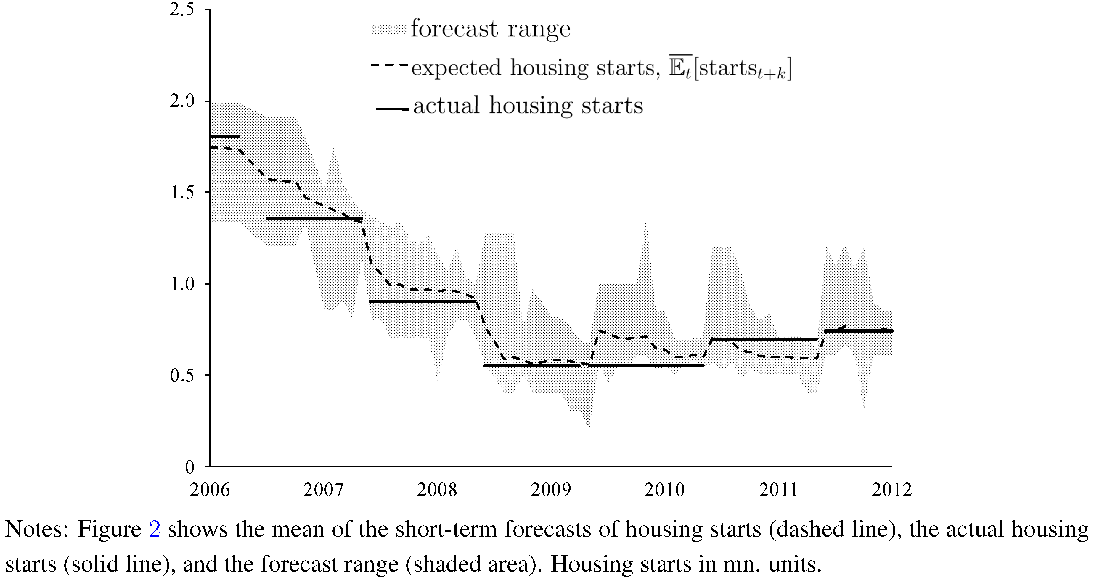
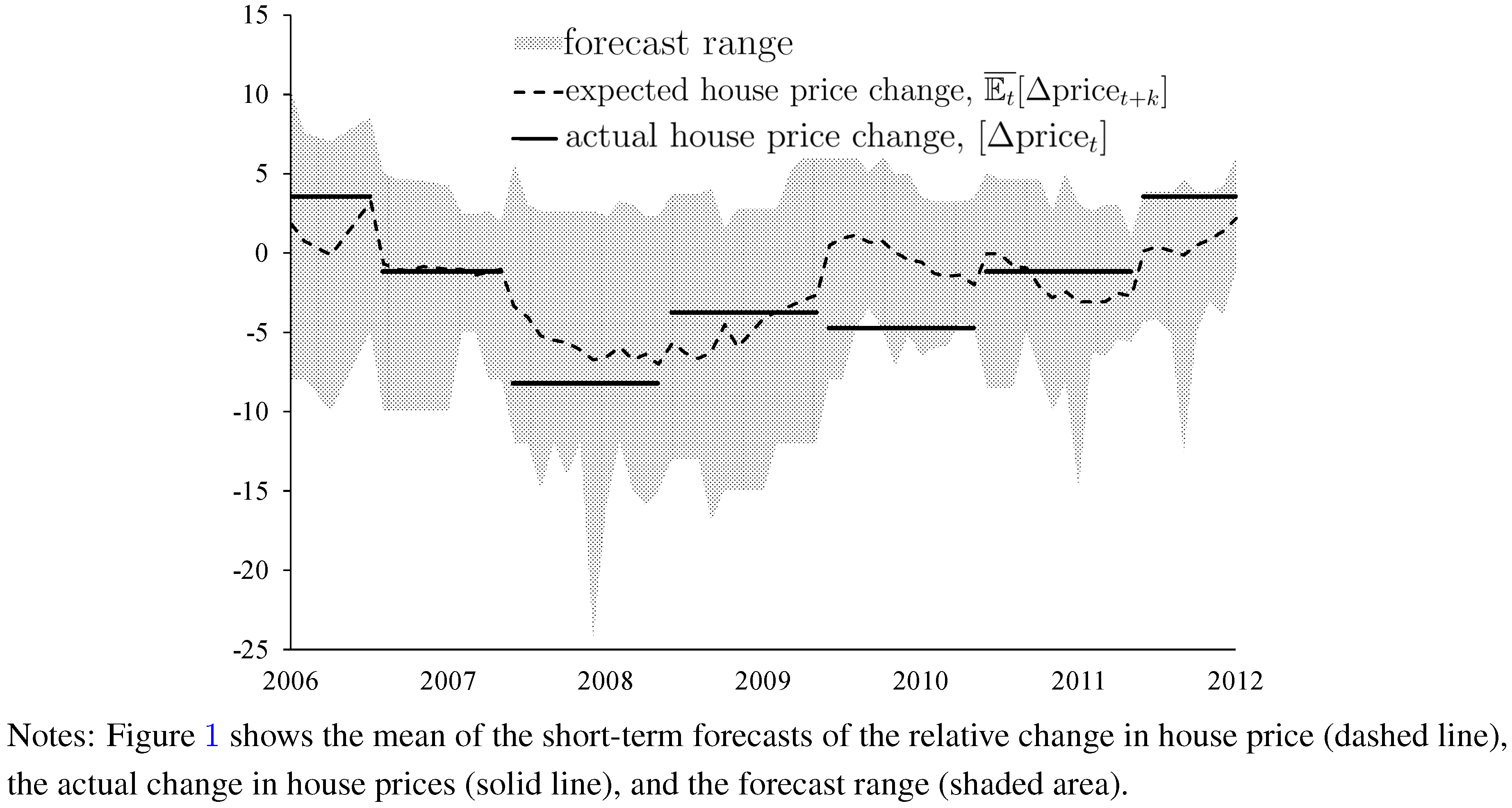
Figure 1 (change in house prices) and Figure 2 (housing starts) illustrate that one should not only focus on the cross-sectional, time-averaged mean values of forecasts. A characteristic feature of the WSJ data is that forecasts witness a characteristic cross-sectional dispersion of forecasts of both changes in house price and housing starts. In Figure 1 and Figure 2, the cross-sectional heterogeneity of forecasts is measured in terms of the cross-sectional range of forecasts (shaded areas). Cross-sectional dispersion of forecasts of, for example, exchange rates has been widely documented in recent literature (see, for example [19]). Pierdzioch et al. [10,11] have documented cross-sectional dispersion of forecasts of housing starts and housing approvals. To the best of our knowledge, the cross-sectional dispersion of forecasts of changes in house prices has not been documented in earlier literature. Given the substantial cross-sectional dispersion of the WSJ data, we used in our empirical analysis individual forecasts of changes in house prices and housing starts rather than cross-sectional mean values.

Table 1. Summary Statistics of the Survey Data (2006–2012).

Panel A: Forecasts of House Prices (percentage change p.a.)
	Short-Term	Medium-Term	Actual
Mean	–2.259	0.134	–2.626
Standard Deviation	(0.066)	(0.060)	(0.055)
Observations	3,524	3,171	68
Panel B: Forecasts of Housing Starts (in million units)
	Short-Term	Medium-Term	Actual
Mean	0.884	1.031	0.840
Standard Deviation	(0.006)	(0.006)	(0.005)
Observations	3,648	3,240	68

Note: The short-term (medium-term) forecasts refer to the forecasts for the current (next) year. The actual values were taken from Federal Housing Finance Agency.

Table 1. Summary Statistics of the Survey Data (2006–2012).

Panel A: Forecasts of House Prices (percentage change p.a.)
	Short-Term	Medium-Term	Actual
Mean	–2.259	0.134	–2.626
Standard Deviation	(0.066)	(0.060)	(0.055)
Observations	3,524	3,171	68
Panel B: Forecasts of Housing Starts (in million units)
	Short-Term	Medium-Term	Actual
Mean	0.884	1.031	0.840
Standard Deviation	(0.006)	(0.006)	(0.005)
Observations	3,648	3,240	68

Note: The short-term (medium-term) forecasts refer to the forecasts for the current (next) year. The actual values were taken from Federal Housing Finance Agency.

Figure 1. Expected and Actual Change in House Prices.

Figure 1. Expected and Actual Change in House Prices.

In addition to the cross-sectional dispersion of the WSJ data, Figure 1 and Figure 2 plot time series of (i) the cross-sectional mean values of the forecasts of changes in house prices and forecasts of housing starts (dashed lines); and, (ii) the actual relative change in house prices and the actual housing starts (solid lines). The cross-sectional mean values of changes in house prices and housing starts move in tandem with the respective actual values, at least as results for end-of-year values are concerned. This result is in line with economic intuition because forecast accuracy should increase as the forecast horizon decreases.

Figure 2. Expected and Actual Housing Starts.

Figure 2. Expected and Actual Housing Starts.

3. (Anti-)Herding of Forecasters

The significant cross-sectional dispersion of forecasts of changes in house prices and of forecasts of housing starts gives rise to the question whether herding (or anti-herding) of forecasters helps to explain this dispersion. Herding of forecasters arises if forecasters deliberately center their forecasts around a consensus forecast. The consensus forecast can be represented by the cross-sectional mean of the forecasts made by forecasters who participate, in a given forecasting cycle, in a questionnaire survey. Anti-herding, in contrast, arises if forecasts try to differentiate forecasts by deliberately placing their forecast farther away from the consensus forecast. This definition of forecaster (anti-) herding should make clear that our analysis concerns the cross-sectional herding (or anti-herding) of forecasters. In earlier empirical research, researchers have used the term “herding” to characterize the time-series properties of forecasts. Our use of the term herding, thus, should not be confused with the terminology used by other researchers who have used the term herding to describe, for example, trend-extrapolative forecasts in a time-series context.

We used a test that has recently been developed by Bernhardt et al. [2] to analyze whether forecasters (anti-)herd. Using this test ensures that our results can be readily compared with results reported recently by Pierdzioch et al. [10,11]. The test is easy to implement, the economic interpretation of the test results is straightforward, and the test is robust to various types of specification errors. The mechanics of the test can be illustrated by considering a forecaster who forms an efficient private forecast of house prices or housing starts. The forecaster derives her private forecast by applying her optimal forecasting model, and by using all information available to her at the time she forms the forecast. Her private forecast, thus, should be unbiased, and the probability that her unbiased private forecast overshoots or undershoots the future house price should be .

The published forecast may differ from the private forecast if the published forecast is influenced by the consensus forecast. In the case of herding, a forecaster places her published forecast closer to the consensus forecast than warranted by her private forecast. The published forecast will be biased towards the consensus forecast. In case the private forecast exceeds the consensus forecast, the published forecast thus will be smaller than the private forecast. The probability of undershooting is then smaller than 0.5. In a similar vein, if the private forecast is smaller than the consensus forecast, the probability that future house prices or future housing starts overshoot the published forecast is also smaller than 0.5. In contrast, in the case of anti-herding, the published forecast will be farther away from the consensus forecast than the private forecast. The result is that the probability of undershooting and the probability of overshooting will be larger than 0.5.

The probabilities of undershooting and overshooting (computed as the relative frequencies of events, using data for all forecasters) can be used to develop a simple test of herding and anti-herding. Under the null hypothesis that forecasters neither herd nor anti-herd, the probability, , that forecasts of future house prices or housing starts ( , where is a forecaster index) overshoot (undershoot) future house prices or housing starts ( ) should be 0.5, regardless of the consensus forecast ( ). The conditional probability of undershooting in the case forecasts exceed the consensus forecast should be

(1)

and the conditional probability of overshooting in the case forecasts are smaller than the consensus forecast should be

(2)

In the case of herding, published forecasts will center around the consensus forecast, implying that the conditional probabilities should be smaller than 0.5. In the case of anti-herding, the published forecasts will be farther away from the consensus forecast, and the conditional probabilities should be larger than 0.5. The test statistic, , defined as the arithmetic average of the sample estimates of the two conditional probabilities, should assume the value in the case case of unbiased forecasts, the value in the case of herding, and the value in the case of anti-herding. (For a graphical illustration of how forecaster (anti-)herding affects the undershooting and overshooting probabilities, See Pierdzioch et al. [4].) Bernhardt et al. [2] show that the test statistic , asymptotically has a normal sampling distribution. They also demonstrate that, due to the averaging of conditional probabilities, the test statistic, , is robust to phenomena like, for example, correlated forecast errors and optimism or pessimism among forecasters. Such phenomena make it more difficult to reject the null hypothesis of unbiased forecasts.

The results summarized in Table 2 show that the test statistic, , significantly exceeds the value , providing strong evidence of forecaster anti-herding. (The number of observations is slightly smaller than in Table 1 because some forecasts are equal to the subsequently realized value, that is, . Equations (1) and (2) show that such forecasts were dropped from the analysis.) The evidence of anti-herding is strong regardless of the forecast horizon and regardless of whether we studied forecasts of changes in house prices or housing starts. We computed the test statistic, , using the consensus of the previous period, , because forecasters deliver their forecasts simultaneously, implying that the contemporaneous consensus forecast may not be in forecasters information set. More precisely, we used the forecast from the predecessor survey to compute the consensus forecast. As for January forecasts, we used the medium-term December forecasts to compute the consensus forecast. (We also found strong evidence of forecaster anti-herding when we used the contemporaneous consensus forecast to compute the test statistic, . Results are not reported, but available upon request.)

Table 2. Test for Herding.

Panel A: Short-Term Forecasts of House Prices
	633 / 35.1 %	1,341 / 78.3 %
	1,171 / 64.9 %	371 / 21.7 %
Sum	1,804 / 100.0 %	1,712 / 100.0 %
S-Stat	0.716
Stand. Error	0.0084
Lower 99 %	0.694
Upper 99 %	0.738
Observations	3,516
Panel B: Medium-Term Forecasts of House Price
	795 / 57.4 %	1,341 / 85.3 %
	589 / 42.6 %	232 / 14.7 %
Sum	1,384 / 100.0 %	1,573 / 100.0 %
S-Stat	0.639
Stand. Error	0.0092
Lower 99 %	0.615
Upper 99 %	0.663
Observations	2,957
Panel C: Short-Term Forecasts of Housing Starts
	972 / 49.4 %	1,266 / 85.3 %
	995 / 50.6 %	219 / 14.7 %
Sum	1,967 / 100.0 %	1,485 / 100.0 %
S-Stat	0.679
Stand. Error	0.0086
Lower 99 %	0.657
Upper 99 %	0.702
Observations	3,452
Panel D: Medium-Term Forecasts of Housing Starts
	1,153 / 72.8 %	1,336 / 96.6 %
	430 / 27.2 %	47 / 3.4 %
Sum	1,583 / 100.0 %	1,383 / 100.0 %
S-Stat	0.619
Stand. Error	0.0092
Lower 99 %	0.595
Upper 99 %	0.643
Observations	2,966

Table 2. Test for Herding.

Panel A: Short-Term Forecasts of House Prices
	633 / 35.1 %	1,341 / 78.3 %
	1,171 / 64.9 %	371 / 21.7 %
Sum	1,804 / 100.0 %	1,712 / 100.0 %
S-Stat	0.716
Stand. Error	0.0084
Lower 99 %	0.694
Upper 99 %	0.738
Observations	3,516
Panel B: Medium-Term Forecasts of House Price
	795 / 57.4 %	1,341 / 85.3 %
	589 / 42.6 %	232 / 14.7 %
Sum	1,384 / 100.0 %	1,573 / 100.0 %
S-Stat	0.639
Stand. Error	0.0092
Lower 99 %	0.615
Upper 99 %	0.663
Observations	2,957
Panel C: Short-Term Forecasts of Housing Starts
	972 / 49.4 %	1,266 / 85.3 %
	995 / 50.6 %	219 / 14.7 %
Sum	1,967 / 100.0 %	1,485 / 100.0 %
S-Stat	0.679
Stand. Error	0.0086
Lower 99 %	0.657
Upper 99 %	0.702
Observations	3,452
Panel D: Medium-Term Forecasts of Housing Starts
	1,153 / 72.8 %	1,336 / 96.6 %
	430 / 27.2 %	47 / 3.4 %
Sum	1,583 / 100.0 %	1,383 / 100.0 %
S-Stat	0.619
Stand. Error	0.0092
Lower 99 %	0.595
Upper 99 %	0.643
Observations	2,966

To analyze the impact of the Lehman collapse on expectation formation in the housing market, we split the sample period into two subsample periods in Table 3 and Table 4: a pre-Lehman collapse subsample period, and a post-Lehman collapse subsample period. The results confirm that forecasters of changes in house prices anti-herd before and after the Lehman collapse. Interestingly, forecaster anti-herding tends to be more pronounced in the period before the Lehman collapse with regard to housing starts. For medium-term forecasts of housing starts, the herding statistic even becomes only marginally significant in the post-Lehman sample. While the interpretation of this result should not be stretched too far, it may reflect that the strategic interactions between forecasters of housing starts have become weaker after the collapse of Lehman brothers, and after the housing rally pricked.

Table 3. Test for Herding before Lehman.

Panel A: Short-Term Forecasts of House Prices
	463 / 36.7 %	795 / 72.1 %
	798 / 63.3 %	308 / 27.9 %
Sum	1,261 / 100.0 %	1,103 / 100.0 %
S-Stat	0.677
Stand. Error	0.0103
Lower 99 %	0.650
Upper 99 %	0.704
Observations	2,364
Panel B: Medium-Term Forecasts of House Price
	408 / 47.1 %	779 / 77.4 %
	459 / 52.9 %	228 / 22.6 %
Sum	867 / 100.0 %	1,007 / 100.0 %
S-Stat	0.651
Stand. Error	0.0116
Lower 99 %	0.621
Upper 99 %	0.682
Observations	1,874
Panel C: Short-Term Forecasts of Housing Starts
	632 / 45.2 %	797 / 84.1 %
	767 / 54.8 %	151 / 15.9 %
Sum	1,399 / 100.0 %	948 / 100.0 %
S-Stat	0.694
Stand. Error	0.0105
Lower 99 %	0.667
Upper 99 %	0.722
Observations	2,347
Panel D: Medium-Term Forecasts of Housing Starts
	647 / 60.9 %	776 / 94.3 %
	415 / 39.1 %	47 / 5.7 %
Sum	1,062 / 100.0 %	823 / 100.0 %
S-Stat	0.667
Stand. Error	0.0116
Lower 99 %	0.636
Upper 99 %	0.697
Observations	1,885

Table 3. Test for Herding before Lehman.

Panel A: Short-Term Forecasts of House Prices
	463 / 36.7 %	795 / 72.1 %
	798 / 63.3 %	308 / 27.9 %
Sum	1,261 / 100.0 %	1,103 / 100.0 %
S-Stat	0.677
Stand. Error	0.0103
Lower 99 %	0.650
Upper 99 %	0.704
Observations	2,364
Panel B: Medium-Term Forecasts of House Price
	408 / 47.1 %	779 / 77.4 %
	459 / 52.9 %	228 / 22.6 %
Sum	867 / 100.0 %	1,007 / 100.0 %
S-Stat	0.651
Stand. Error	0.0116
Lower 99 %	0.621
Upper 99 %	0.682
Observations	1,874
Panel C: Short-Term Forecasts of Housing Starts
	632 / 45.2 %	797 / 84.1 %
	767 / 54.8 %	151 / 15.9 %
Sum	1,399 / 100.0 %	948 / 100.0 %
S-Stat	0.694
Stand. Error	0.0105
Lower 99 %	0.667
Upper 99 %	0.722
Observations	2,347
Panel D: Medium-Term Forecasts of Housing Starts
	647 / 60.9 %	776 / 94.3 %
	415 / 39.1 %	47 / 5.7 %
Sum	1,062 / 100.0 %	823 / 100.0 %
S-Stat	0.667
Stand. Error	0.0116
Lower 99 %	0.636
Upper 99 %	0.697
Observations	1,885

Table 4. Test for Herding after Lehman collapse.

Panel A: Short-Term Forecasts of House Prices
	172 / 31.6 %	544 / 89.5 %
	372 / 68.4 %	64 / 10.5 %
Sum	544 / 100.0 %	608 / 100.0 %
S-Stat	0.789
Stand. Error	0.0148
Lower 99 %	0.751
Upper 99 %	0.828
Observations	1,152
Panel B: Medium-Term Forecasts of House Price
	385 / 74.2 %	564 / 100.0 %
	134 / 25.8 %	0 / 0.0 %
Sum	519 / 100.0 %	564 / 100.0 %
S-Stat	0.629
Stand. Error	0.0152
Lower 99 %	0.589
Upper 99 %	0.669
Observations	1,083
Panel C: Short-Term Forecasts of Housing Starts
	333 / 59.8 %	476 / 86.9 %
	224 / 40.2 %	72 / 13.1 %
Sum	557 / 100.0 %	548 / 100.0 %
S-Stat	0.635
Stand. Error	0.0150
Lower 99 %	0.596
Upper 99 %	0.675
Observations	1,105
Panel D: Medium-Term Forecasts of Housing Starts
	453 / 88.0 %	566 / 100.0 %
	62 / 12.0 %	0 / 0.0 %
Sum	515 / 100.0 %	566 / 100.0 %
S-Stat	0.560
Stand. Error	0.0152
Lower 99 %	0.520
Upper 99 %	0.600
Observations	1,081

Table 4. Test for Herding after Lehman collapse.

Panel A: Short-Term Forecasts of House Prices
	172 / 31.6 %	544 / 89.5 %
	372 / 68.4 %	64 / 10.5 %
Sum	544 / 100.0 %	608 / 100.0 %
S-Stat	0.789
Stand. Error	0.0148
Lower 99 %	0.751
Upper 99 %	0.828
Observations	1,152
Panel B: Medium-Term Forecasts of House Price
	385 / 74.2 %	564 / 100.0 %
	134 / 25.8 %	0 / 0.0 %
Sum	519 / 100.0 %	564 / 100.0 %
S-Stat	0.629
Stand. Error	0.0152
Lower 99 %	0.589
Upper 99 %	0.669
Observations	1,083
Panel C: Short-Term Forecasts of Housing Starts
	333 / 59.8 %	476 / 86.9 %
	224 / 40.2 %	72 / 13.1 %
Sum	557 / 100.0 %	548 / 100.0 %
S-Stat	0.635
Stand. Error	0.0150
Lower 99 %	0.596
Upper 99 %	0.675
Observations	1,105
Panel D: Medium-Term Forecasts of Housing Starts
	453 / 88.0 %	566 / 100.0 %
	62 / 12.0 %	0 / 0.0 %
Sum	515 / 100.0 %	566 / 100.0 %
S-Stat	0.560
Stand. Error	0.0152
Lower 99 %	0.520
Upper 99 %	0.600
Observations	1,081

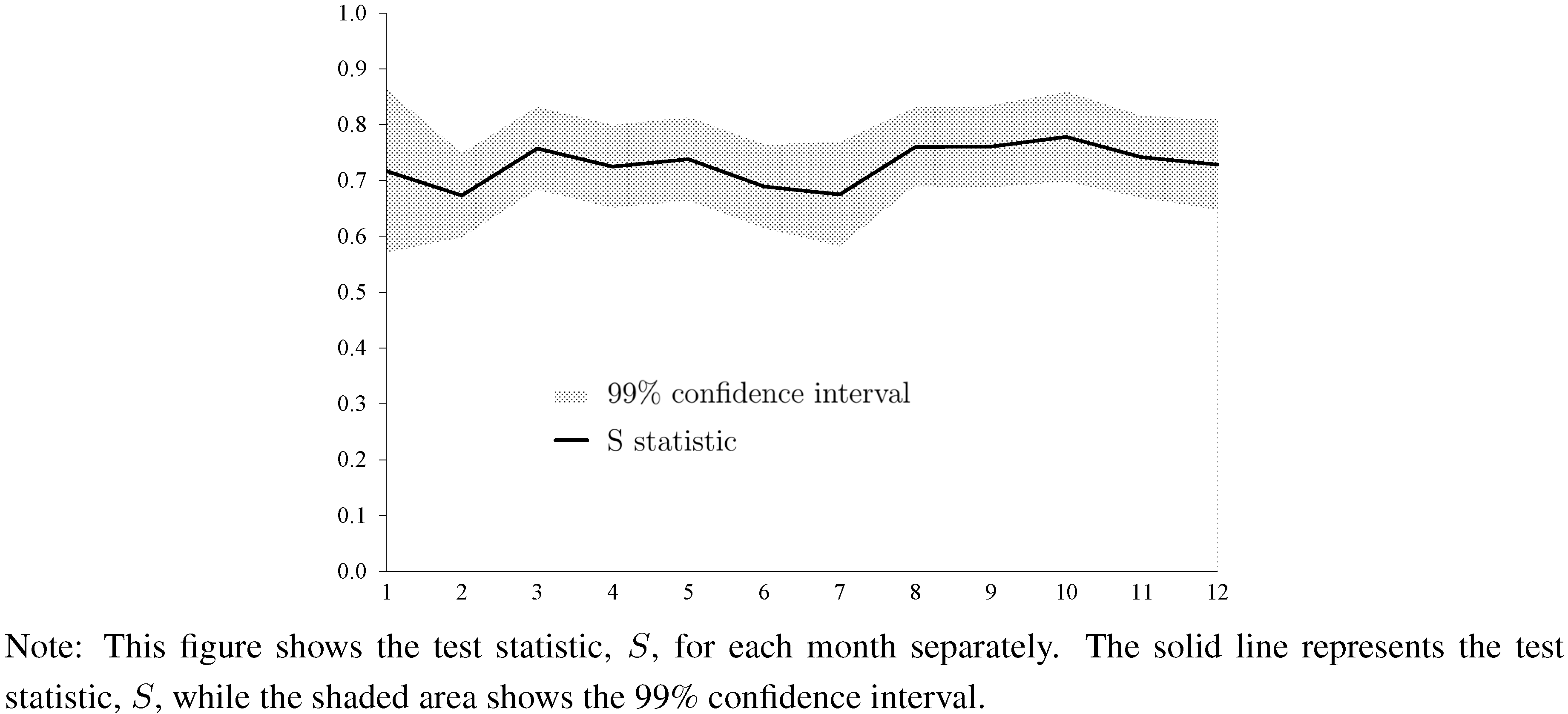
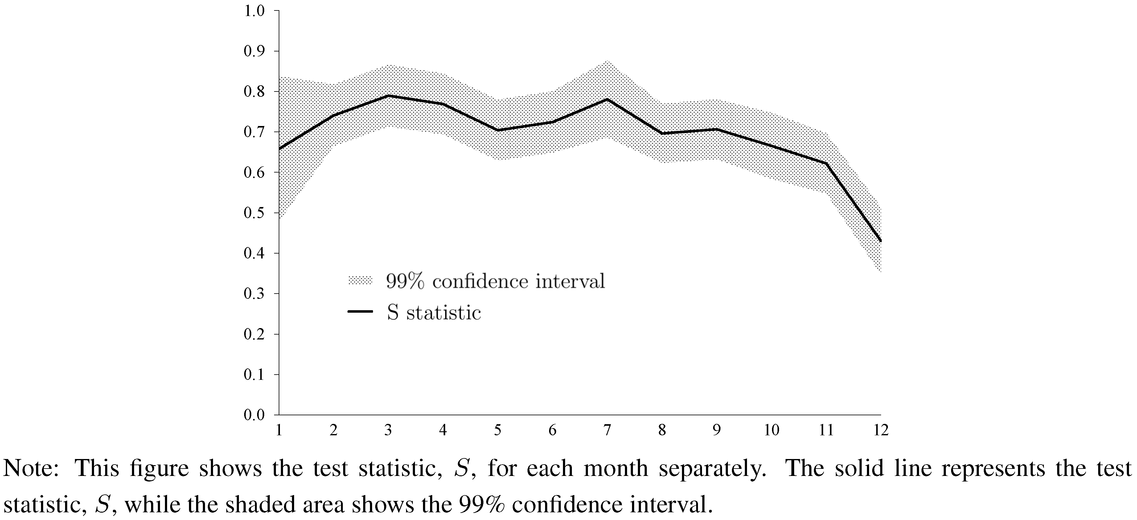
As yet another robustness test, we tested whether forecaster (anti-)herding is stable over the forecasting cycle. To this end, we computed the test statistic, , for each month separately (that is, for forecasts made in January, forecasts made in February, ...), where we used data from the previous month to compute the consensus forecast. Figure 3 and Figure 4 report the results based on the current-year forecasts. (We do not present results for the next-year forecasts because we do not have a consensus forecast for next-year forecasts in January. Results for next-year forecasts are qualitatively similar and are available upon request.) Results show strong evidence of forecaster anti-herding for all months in the case of forecasts of house price changes. The test statistic, , always settles above the 0.5 line. Concerning current-year forecasts of housing starts, we also find strong evidence of forecaster anti-herding, but the results are somewhat more variable across months as compared with forecasts of changes of house prices. December forecasts are not significantly different from 0.5.

Figure 3. Test Statistic for Every Month (Changes of House Prices, Current-Year Forecasts).

Figure 3. Test Statistic for Every Month (Changes of House Prices, Current-Year Forecasts).

Figure 4. Test Statistic for Every Month (Housing Starts, Current-Year Forecasts).

Figure 4. Test Statistic for Every Month (Housing Starts, Current-Year Forecasts).

4. Concluding Remarks

We have used the monthly WSJ survey data on forecasts of changes in house prices and housing starts to analyze (anti-)herding of forecasters during the recent U.S. subprime mortgage crisis. Confirming results of recent research, our results show that anti-herding was prevalent among forecasters. This also holds for forecasts of changes in house prices, which have not been studied in recent research on forecaster anti-herding. In conjunction with results reported in earlier research for different data sets, our results for the WSJ survey data suggest that, in contrast to conventional wisdom, anti-herding prevails among forecasters of housing markets. Our results further indicate that, depending on the variable being forecasted, the extent of forecaster anti-herding may have changed over time. In particular, our results imply that, after the collapse of Lehman brothers, forecaster anti-herding may have become less prevalent with regard to forecasts of housing starts. Forecasts of changes in house prices, however, show strong signs of forecaster anti-herding even in the subsample period following the Lehman collapse.

In economic terms, it may be the case that the prevalence of forecaster anti-herding reflects changing demand for forecasts during periods of housing booms and housing busts. If demand for forecasts falls during a housing bust, incentives to anti-herd may weaken because potential revenues a forecaster can earn by making an extreme forecast are smaller than during a housing boom. The prevalence of forecaster anti-herding also may respond to changing uncertainty. For example, Bewley and Fiebig [20] find that anti-herding among interest rate forecasters is positively correlated with the volatility of interest rates. It is interesting to study in future research whether a similar correlation between forecaster anti-herding and volatilities of changes in house prices and housing starts can be detected in the data that we have studied in this research.