Raman Imaging of Plant Cell Walls in Sections of Cucumis sativus

 ,
, 
Abstract
:1. Introduction
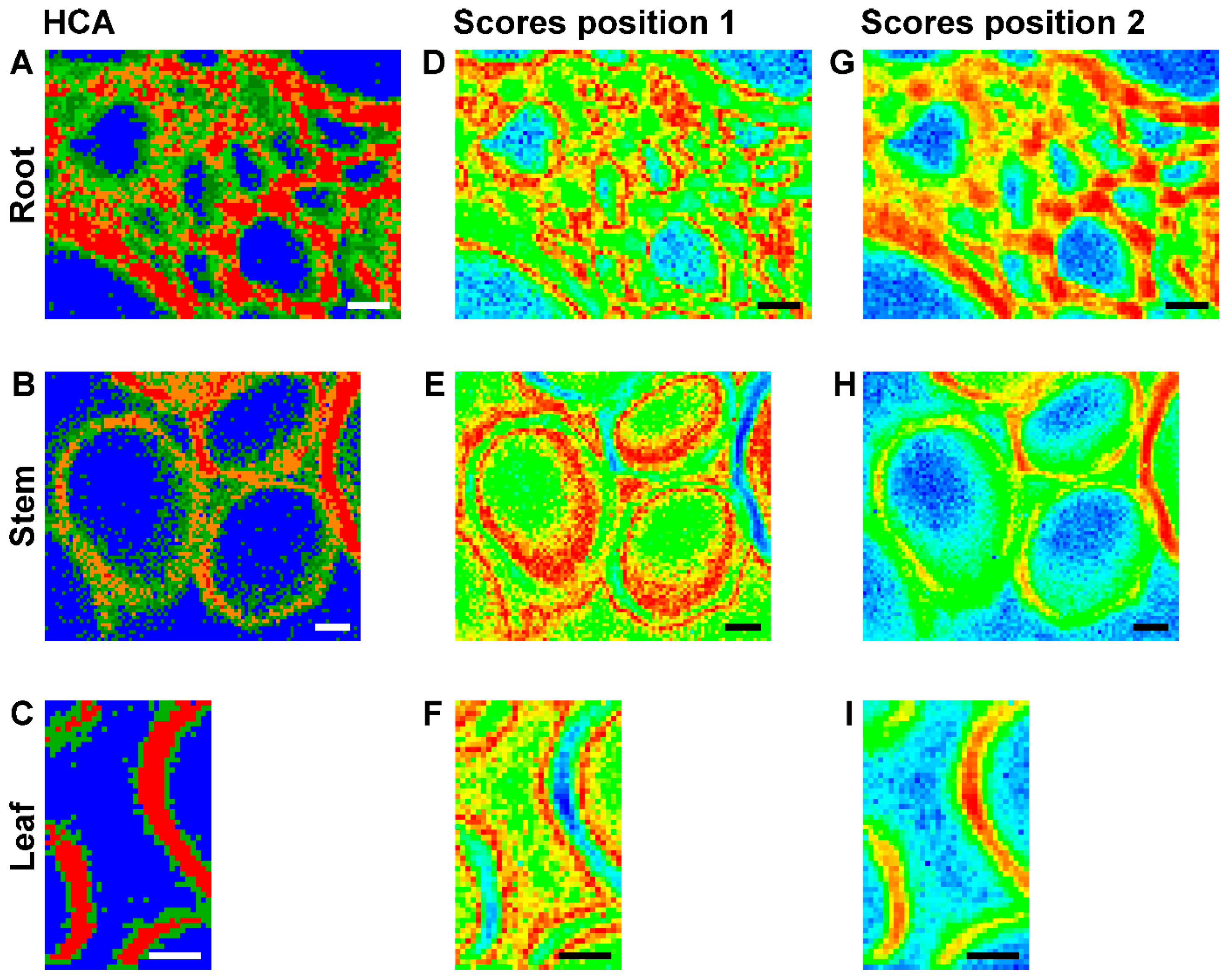
2. Results and Discussion
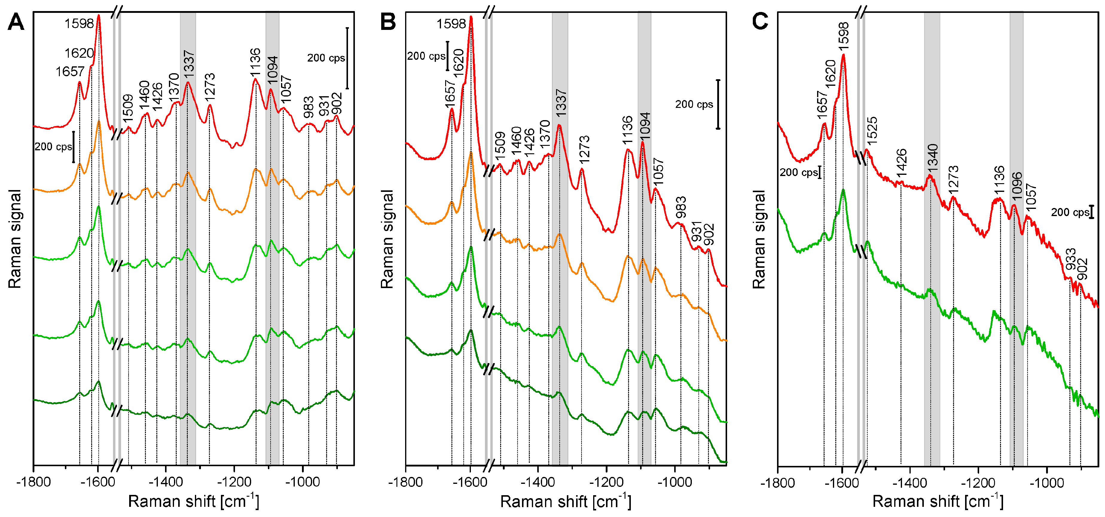
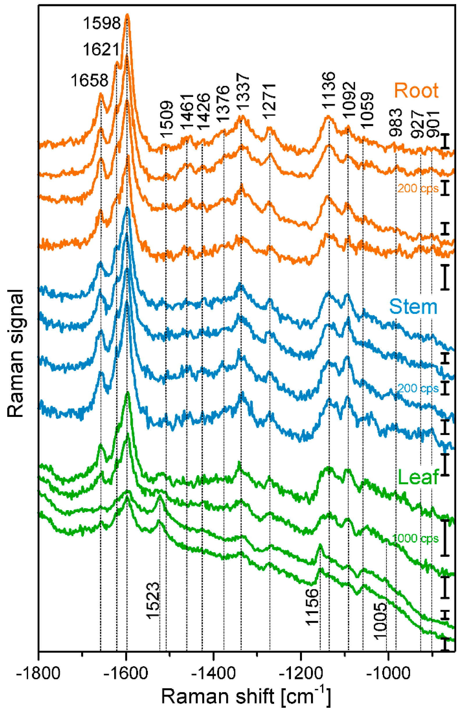
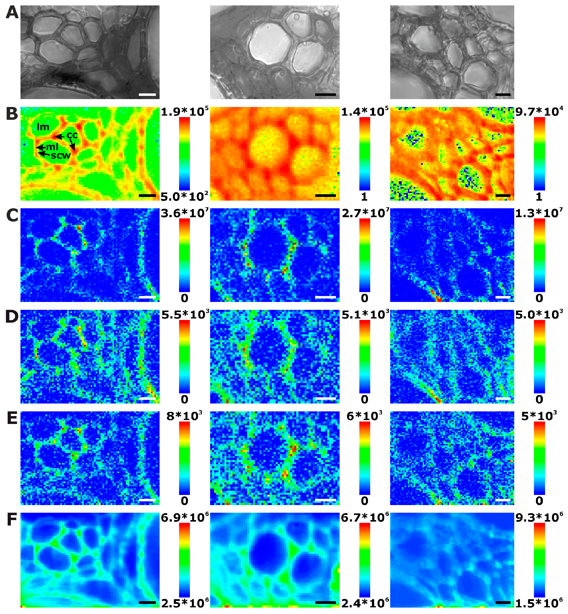
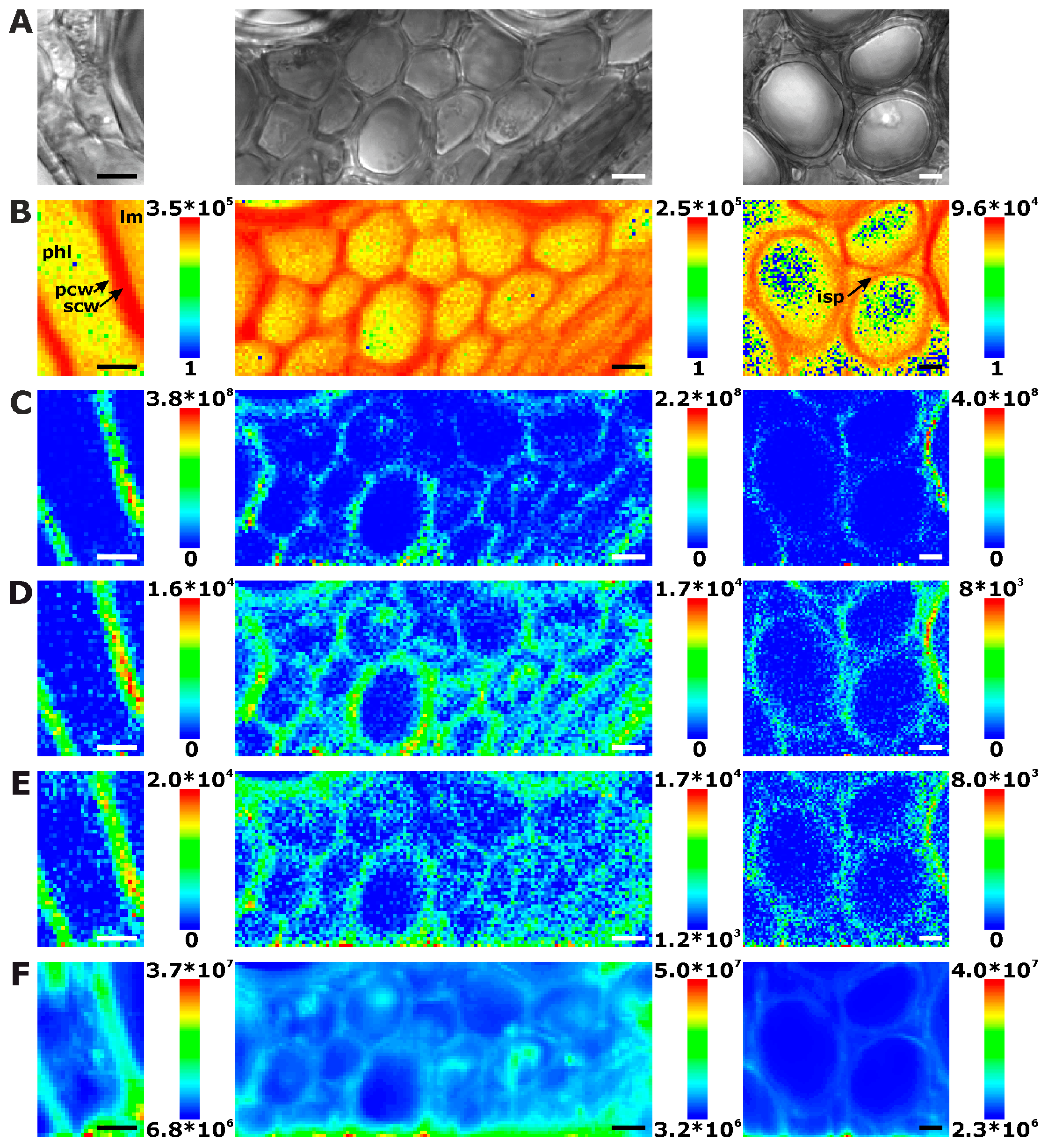
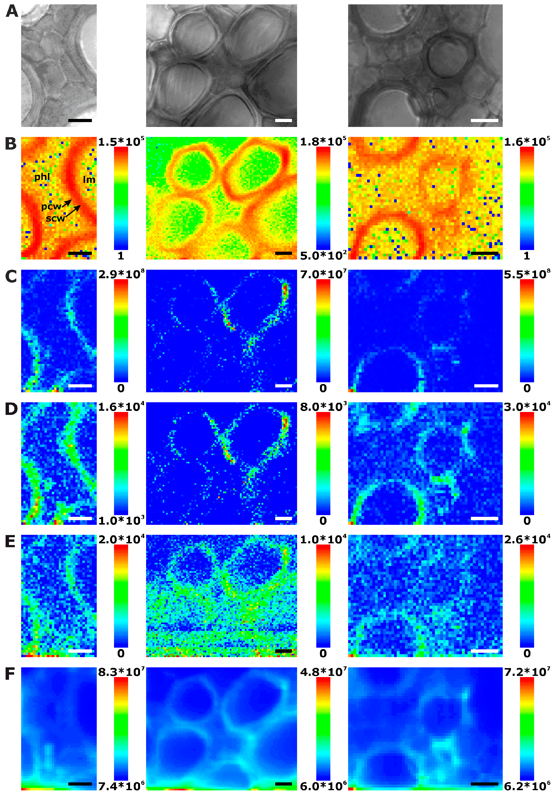
2.1. Histological Information from Chemical Composition
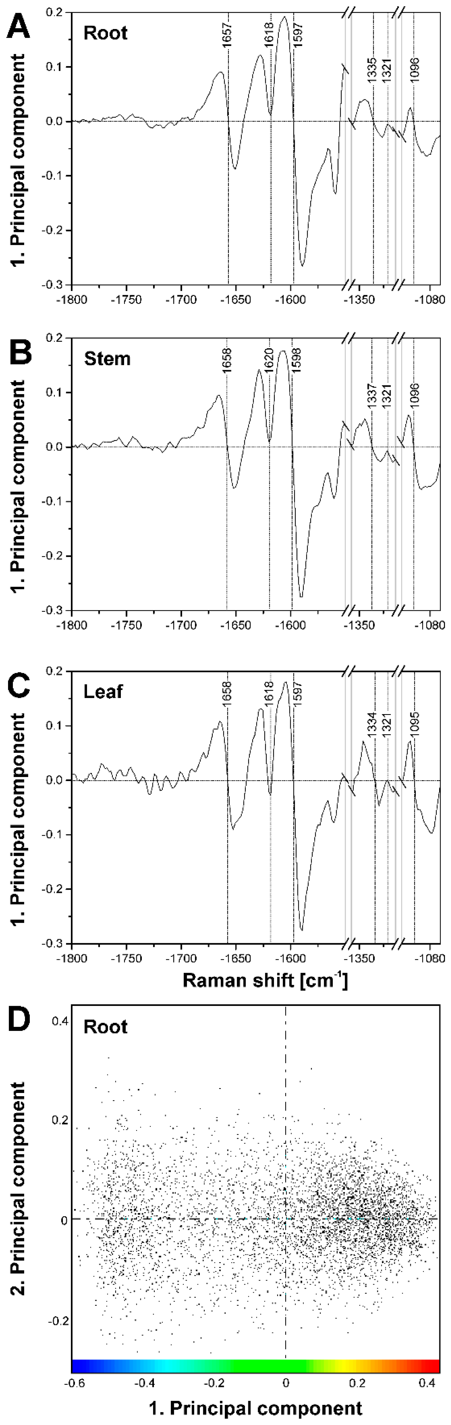
2.2. Improving Image Contrast by Pattern Recognition
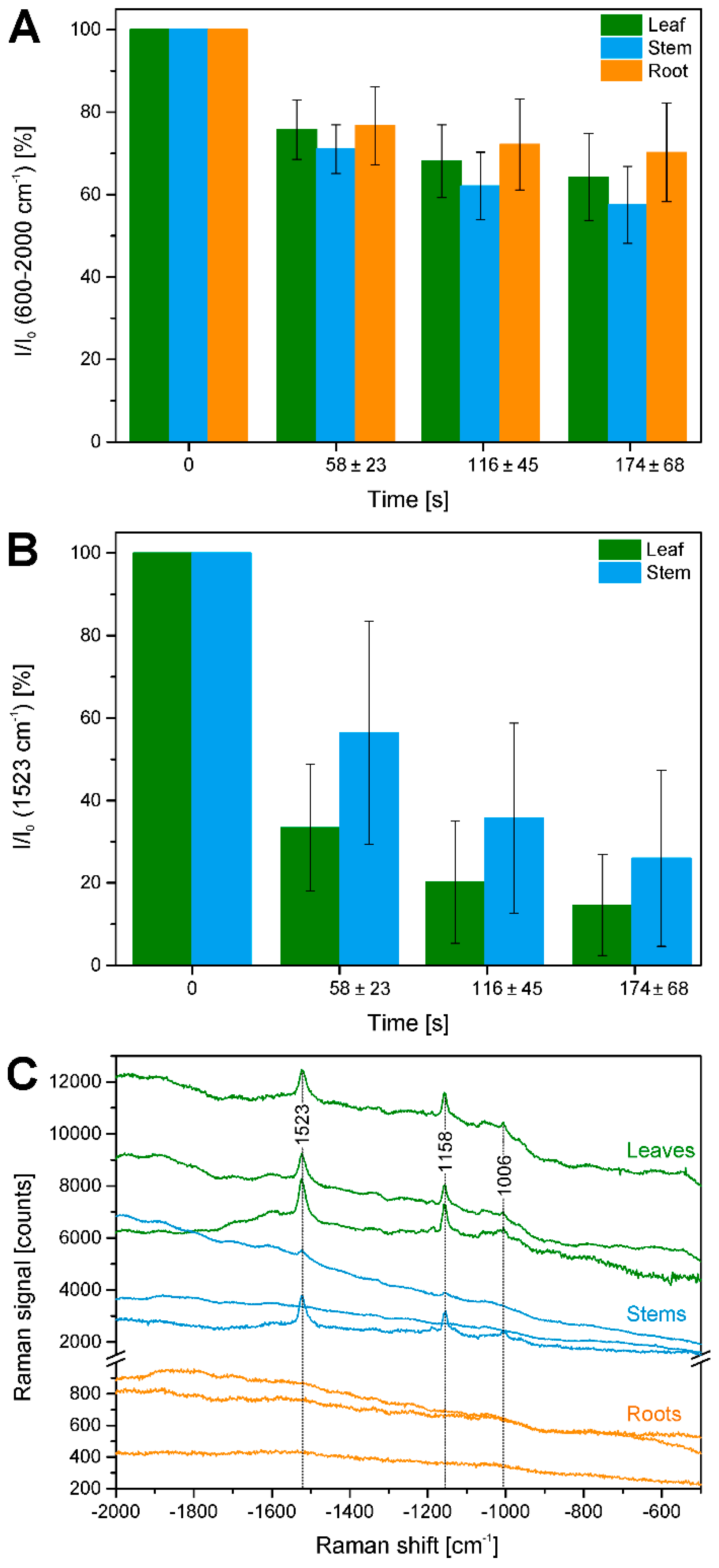
2.3. Bleaching of Photosensitive Molecules
3. Materials and Methods
3.1. Sample Preparation
3.2. Raman Measurements
3.3. Data pre-Processing and Analysis
4. Conclusions
Acknowledgments
Author Contributions
Conflicts of Interest
References
- Schulte, F.; Lingott, J.; Panne, U.; Kneipp, J. Chemical Characterization and Classification of Pollen. Anal. Chem. 2008, 80, 9551–9556. [Google Scholar] [CrossRef] [PubMed]
- Schulte, F.; Panne, U.; Kneipp, J. Molecular changes during pollen germination can be monitored by Raman microspectroscopy. J. Biophotonics 2010, 3, 542–547. [Google Scholar] [CrossRef] [PubMed]
- Schulz, H.; Baranska, M.; Baranski, R. Potential of NIR-FT-Raman spectroscopy in natural carotenoid analysis. Biopolymers 2005, 77, 212–221. [Google Scholar] [CrossRef] [PubMed]
- Lopez-Casado, G.; Matas, A.J.; Dominguez, E.; Cuartero, J.; Heredia, A. Biomechanics of isolated tomato (Solanum lycopersicum L.) fruit cuticles: The role of the cutin matrix and polysaccharides. J. Exp. Bot. 2007, 58, 3875–3883. [Google Scholar] [CrossRef] [PubMed]
- Roman, M.; Dobrowolski, J.C.; Baranska, M.; Baranski, R. Spectroscopic Studies on Bioactive Polyacetylenes and Other Plant Components in Wild Carrot Root. J. Nat. Prod. 2011, 74, 1757–1763. [Google Scholar] [CrossRef] [PubMed]
- Atalla, R.H.; Agarwal, U.P. Raman Microprobe Evidence for Lignin Orientation in the Cell-Walls of Native Woody Tissue. Science 1985, 227, 636–638. [Google Scholar] [CrossRef] [PubMed]
- Agarwal, U.P. Raman imaging to investigate ultrastructure and composition of plant cell walls: Distribution of lignin and cellulose in black spruce wood (Picea mariana). Planta 2006, 224, 1141–1153. [Google Scholar] [CrossRef] [PubMed]
- Gierlinger, N.; Schwanninger, M. Chemical imaging of poplar wood cell walls by confocal Raman microscopy. Plant Physiol. 2006, 140, 1246–1254. [Google Scholar] [CrossRef] [PubMed]
- Schmidt, M.; Schwartzberg, A.M.; Perera, P.N.; Weber-Bargioni, A.; Carroll, A.; Sarkar, P.; Bosneaga, E.; Urban, J.J.; Song, J.; Balakshin, M.Y.; et al. Label-free in situ imaging of lignification in the cell wall of low lignin transgenic Populus trichocarpa. Planta 2009, 230, 589–597. [Google Scholar] [CrossRef] [PubMed]
- Gierlinger, N. Revealing changes in molecular composition of plant cell walls on the micron-level by Raman mapping and vertex component analysis (VCA). Front. Plant Sci. 2014, 5, 306. [Google Scholar] [CrossRef] [PubMed]
- Ma, J.; Zhou, X.; Ma, J.; Ji, Z.; Zhang, X.; Xu, F. Raman Microspectroscopy Imaging Study on Topochemical Correlation Between Lignin and Hydroxycinnamic Acids in Miscanthus sinensis. Microsc. Microanal. 2014, 20, 956–963. [Google Scholar] [CrossRef] [PubMed]
- Baranska, M.; Roman, M.; Dobrowolski, J.C.; Schulz, H.; Baranski, R. Recent Advances in Raman Analysis of Plants: Alkaloids, Carotenoids, and Polyacetylenes. Curr. Anal. Chem. 2013, 9, 108–127. [Google Scholar] [CrossRef]
- Gierlinger, N.; Schwanninger, M. The potential of Raman microscopy and Raman imaging in plant research. Spectroscopy 2007, 21, 69–89. [Google Scholar] [CrossRef]
- Butler, H.J.; McAinsh, M.R.; Adams, S.; Martin, F.L. Application of vibrational spectroscopy techniques to non-destructively monitor plant health and development. Anal. Methods 2015, 7, 4059–4070. [Google Scholar] [CrossRef]
- Heiner, Z.; Zeise, I.; Elbaum, R.; Kneipp, J. Insight into plant cell wall chemistry and structure by combination of multiphoton microscopy with Raman imaging. J. Biophotonics 2017. [Google Scholar] [CrossRef] [PubMed]
- Chylinska, M.; Szymanska-Chargot, M.; Zdunek, A. Imaging of polysaccharides in the tomato cell wall with Raman microspectroscopy. Plant Methods 2014, 10, 14. [Google Scholar] [CrossRef] [PubMed]
- Kanbayashi, T.; Miyafuji, H. Topochemical and morphological characterization of wood cell wall treated with the ionic liquid, 1-ethylpyridinium bromide. Planta 2015, 242, 509–518. [Google Scholar] [CrossRef] [PubMed]
- Schulte, F.; Mader, J.; Kroh, L.W.; Panne, U.; Kneipp, J. Characterization of Pollen Carotenoids with in situ and High-Performance Thin-Layer Chromatography Supported Resonant Raman Spectroscopy. Anal. Chem. 2009, 81, 8426–8433. [Google Scholar] [CrossRef] [PubMed]
- Scholtes-Timmerman, M.; Willemse-Erix, H.; Schut, T.B.; van Belkum, A.; Puppels, G.; Maquelin, K. A novel approach to correct variations in Raman spectra due to photo-bleachable cellular components. Analyst 2009, 134, 387–393. [Google Scholar] [CrossRef] [PubMed]
- Patterson, R.F.; Hibbert, H. Studies on Lignin and Related Compounds. LXXII. The Ultraviolet Absorption Spectra of Compounds Related to Lignin. J. Am. Chem. Soc. 1943, 65, 1862–1869. [Google Scholar] [CrossRef]
- Lagorio, M.G.; Cordon, G.B.; Iriel, A. Reviewing the relevance of fluorescence in biological systems. Photochem. Photobiol. Sci. 2015, 14, 1538–1559. [Google Scholar] [CrossRef] [PubMed]
- Wiley, J.H.; Atalla, R.H. Band assignments in the Raman spectra of celluloses. Carbohydr. Res. 1987, 160, 113–129. [Google Scholar] [CrossRef]
- Agarwal, U.P.; Ralph, S.A. FT-Raman Spectroscopy of Wood: Identifying Contributions of Lignin and Carbohydrate Polymers in the Spectrum of Black Spruce (Picea mariana). Appl. Spectrosc. 1997, 51, 1648–1655. [Google Scholar] [CrossRef]
- Agarwal, U.P. An Overview of Raman Spectroscopy as Applied to Lignocellulosic Materials. In Advances in Lignocellulosics Characterization; Argyropoulos, D.S., Ed.; TAPPI Press: Atlanta, GA, USA, 1999; Chapter 9; pp. 201–225. [Google Scholar]
- Merlin, J.C. Resonance Raman spectroscopy of carotenoids and carotenoid containing systems. Pure Appl. Chem. 1985, 57, 785–792. [Google Scholar] [CrossRef]
- Baranska, M.; Baranski, R.; Schulz, H.; Nothnagel, T. Tissue-specific accumulation of carotenoids in carrot roots. Planta 2006, 224, 1028–1037. [Google Scholar] [CrossRef] [PubMed]
- Tschirner, N.; Schenderlein, M.; Brose, K.; Schlodder, E.; Mroginski, M.A.; Thomsen, C.; Hildebrandt, P. Resonance Raman spectra of [small beta]-carotene in solution and in photosystems revisited: An experimental and theoretical study. Phys. Chem. Chem. Phys. 2009, 11, 11471–11478. [Google Scholar] [CrossRef] [PubMed]
- Agarwal, U.P.; Atalla, R.H. Insitu Raman Microprobe Studies of Plant-Cell Walls—Macromolecular Organization and Compositional Variability in the Secondary Wall of Picea-Mariana (Mill) Bsp. Planta 1986, 169, 325–332. [Google Scholar] [CrossRef] [PubMed]
- Gierlinger, N.; Luss, S.; Konig, C.; Konnerth, J.; Eder, M.; Fratzl, P. Cellulose microfibril orientation of Picea abies and its variability at the micron-level determined by Raman imaging. J. Exp. Bot. 2010, 61, 587–595. [Google Scholar] [CrossRef] [PubMed]
- Ji, Z.; Ma, J.F.; Zhang, Z.H.; Xu, F.; Sun, R.C. Distribution of lignin and cellulose in compression wood tracheids of Pinus yunnanensis determined by fluorescence microscopy and confocal Raman microscopy. Ind. Crops Prod. 2013, 47, 212–217. [Google Scholar] [CrossRef]
- Sun, L.; Singh, S.; Joo, M.; Vega-Sanchez, M.; Ronald, P.; Simmons, B.A.; Adams, P.; Auer, M. Non-invasive imaging of cellulose microfibril orientation within plant cell walls by polarized Raman microspectroscopy. Biotechnol. Bioeng. 2016, 113, 82–90. [Google Scholar] [CrossRef] [PubMed]
- Agarwal, U.P.; Atalla, R.H. Raman Spectroscopic Evidence for Coniferyl Alcohol Structures in Bleached and Sulfonated Mechanical Pulps. In Photochemistry of Lignocellulosic Materials; American Chemical Society: Washington, DC, USA, 1993; Volume 531, pp. 26–44. [Google Scholar]
- Sun, L.; Varanasi, P.; Yang, F.; Loqué, D.; Simmons, B.A.; Singh, S. Rapid determination of syringyl: Guaiacyl ratios using FT-Raman spectroscopy. Biotechnol. Bioeng. 2012, 109, 647–656. [Google Scholar] [CrossRef] [PubMed]
- Liu, B.; Wang, P.; Kim, J.I.; Zhang, D.; Xia, Y.; Chapple, C.; Cheng, J.-X. Vibrational Fingerprint Mapping Reveals Spatial Distribution of Functional Groups of Lignin in Plant Cell Wall. Anal. Chem. 2015, 87, 9436–9442. [Google Scholar] [CrossRef] [PubMed]
- Donaldson, L.; Radotić, K.; Kalauzi, A.; Djikanović, D.; Jeremić, M. Quantification of compression wood severity in tracheids of Pinus radiata D. Don using confocal fluorescence imaging and spectral deconvolution. J. Struct. Biol. 2010, 169, 106–115. [Google Scholar] [CrossRef] [PubMed]
- Seifert, S.; Merk, V.; Kneipp, J. Identification of aqueous pollen extracts using surface enhanced Raman scattering (SERS) and pattern recognition methods. J. Biophotonics 2016, 9, 181–189. [Google Scholar] [CrossRef] [PubMed]
- Joester, M.; Seifert, S.; Emmerling, F.; Kneipp, J. Physiological influence of silica on germinating pollen as shown by Raman spectroscopy. J. Biophotonics 2017, 10, 542–552. [Google Scholar] [CrossRef] [PubMed]
- Perera, P.N.; Schmidt, M.; Schuck, P.J.; Adams, P.D. Blind image analysis for the compositional and structural characterization of plant cell walls. Anal. Chim. Acta 2011, 702, 172–177. [Google Scholar] [CrossRef] [PubMed]
- Nakashima, J.; Mizuno, T.; Takabe, K.; Fujita, M.; Saiki, H. Direct Visualization of Lignifying Secondary Wall Thickenings in Zinnia elegansCells in Culture. Plant Cell Physiol. 1997, 38, 818–827. [Google Scholar] [CrossRef]
- Hafren, J.; Fujino, T.; Itoh, T. Changes in cell wall architecture of differentiating tracheids of Pinus thunbergii during lignification. Plant Cell Physiol. 1999, 40, 532–541. [Google Scholar] [CrossRef]
- Altaner, C.M.; Tokareva, E.N.; Jarvis, M.C.; Harris, P.J. Distribution of (1→4)-β-galactans, arabinogalactan proteins, xylans and (1→3)-β-glucans in tracheid cell walls of softwoods. Tree Physiol. 2010, 30, 782–793. [Google Scholar] [CrossRef] [PubMed]
- Donaldson, L.A.; Knox, J.P. Localization of Cell Wall Polysaccharides in Normal and Compression Wood of Radiata Pine: Relationships with Lignification and Microfibril Orientation. Plant Physiol. 2012, 158, 642–653. [Google Scholar] [CrossRef] [PubMed]
- Willemse, M.T.M. Cell Wall Autofluorescence. In Physico-Chemical Characterisation of Plant Residues for Industrial and Feed Use; Chesson, A., Ørskov, E.R., Eds.; Springer: Dordrecht, The Netherlands, 1989; pp. 50–57. [Google Scholar]
- Tylli, H.; Forsskåhl, I.; Olkkonen, C. The effect of heat and IR radiation on the fluorescence of cellulose. Cellulose 2000, 7, 133–146. [Google Scholar] [CrossRef]
- Demmig-Adams, B.; Adams, W.W. Carotenoid composition in sun and shade leaves of plants with different life forms. Plant Cell Environ. 1992, 15, 411–419. [Google Scholar] [CrossRef]


| Plant Organ | Number of Maps | Number of Different Cells a | Number of Complete Cells b | Extracted Cell Wall Spectra c | Cell Wall Spectra per Complete Cell | Mean Cell Wall Area per Map [%] |
|---|---|---|---|---|---|---|
| Roots | 20 | 187 | 134 | 39,262 | 294 | 67 ± 13 |
| Stems | 18 | 112 | 56 | 30,282 | 538 | 52 ± 13 |
| Leaves | 17 | 71 | 42 | 24,552 | 592 | 44 ± 17 |
| Band Position [cm−1] | Tentative Assignment to Molecule |
|---|---|
| 901 | δ(HCC) and δ(HCO) at C-6, cellulose |
| 927 | ω(CCH), lignin; |
| 983 | ν(CC) and ν(CO), cellulose |
| 1005 | ν3 Methyl rocking, carotenoid |
| 1059 | ν(CC) and ν(CO), cellulose |
| 1092 | ν(CC) and ν(CO), cellulose |
| 1136 | ν(CC) and ν(CO), cellulose |
| 1156 | ν2 C-C, carotenoid |
| 1271 | Aryl-O of Aryl-OH and Aryl-O-CH3; guaiacylring mode (with CO-group)), lignin |
| 1337 | δ(HCC) and δ(HCO) cellulose |
| 1376 | δ(HCC) and δ(HCO), and δ(HOC), cellulose |
| 1426 | δ(O-CH3), δ(CH2), guaiacyl ring, lignin |
| 1461 | δ(O-CH3), CH2 scissoring, guajacyl ring (with C=O group), lignin; δ(HCH) and δ(HOC), cellulose |
| 1509 | νas(Aryl ring), lignin |
| 1523 | ν1 C=C, carotenoid |
| 1598 | νs(Aryl-Ring), lignin |
| 1621 | νconj.(Ring C=C) of coniferylaldehyde, lignin |
| 1658 | νconj.(Ring C=C) of coniferylalcohol, ν(C=O) of coniferylaldehyde, lignin |
© 2018 by the authors. Licensee MDPI, Basel, Switzerland. This article is an open access article distributed under the terms and conditions of the Creative Commons Attribution (CC BY) license (http://creativecommons.org/licenses/by/4.0/).
Share and Cite
Zeise, I.; Heiner, Z.; Holz, S.; Joester, M.; Büttner, C.; Kneipp, J. Raman Imaging of Plant Cell Walls in Sections of Cucumis sativus. Plants 2018, 7, 7. https://doi.org/10.3390/plants7010007
Zeise I, Heiner Z, Holz S, Joester M, Büttner C, Kneipp J. Raman Imaging of Plant Cell Walls in Sections of Cucumis sativus. Plants. 2018; 7(1):7. https://doi.org/10.3390/plants7010007
Chicago/Turabian StyleZeise, Ingrid, Zsuzsanna Heiner, Sabine Holz, Maike Joester, Carmen Büttner, and Janina Kneipp. 2018. "Raman Imaging of Plant Cell Walls in Sections of Cucumis sativus" Plants 7, no. 1: 7. https://doi.org/10.3390/plants7010007
APA StyleZeise, I., Heiner, Z., Holz, S., Joester, M., Büttner, C., & Kneipp, J. (2018). Raman Imaging of Plant Cell Walls in Sections of Cucumis sativus. Plants, 7(1), 7. https://doi.org/10.3390/plants7010007