
An In Situ Electrical Impedance Tomography Sensor System for Biomass Estimation of Tap Roots


Abstract
:1. Introduction
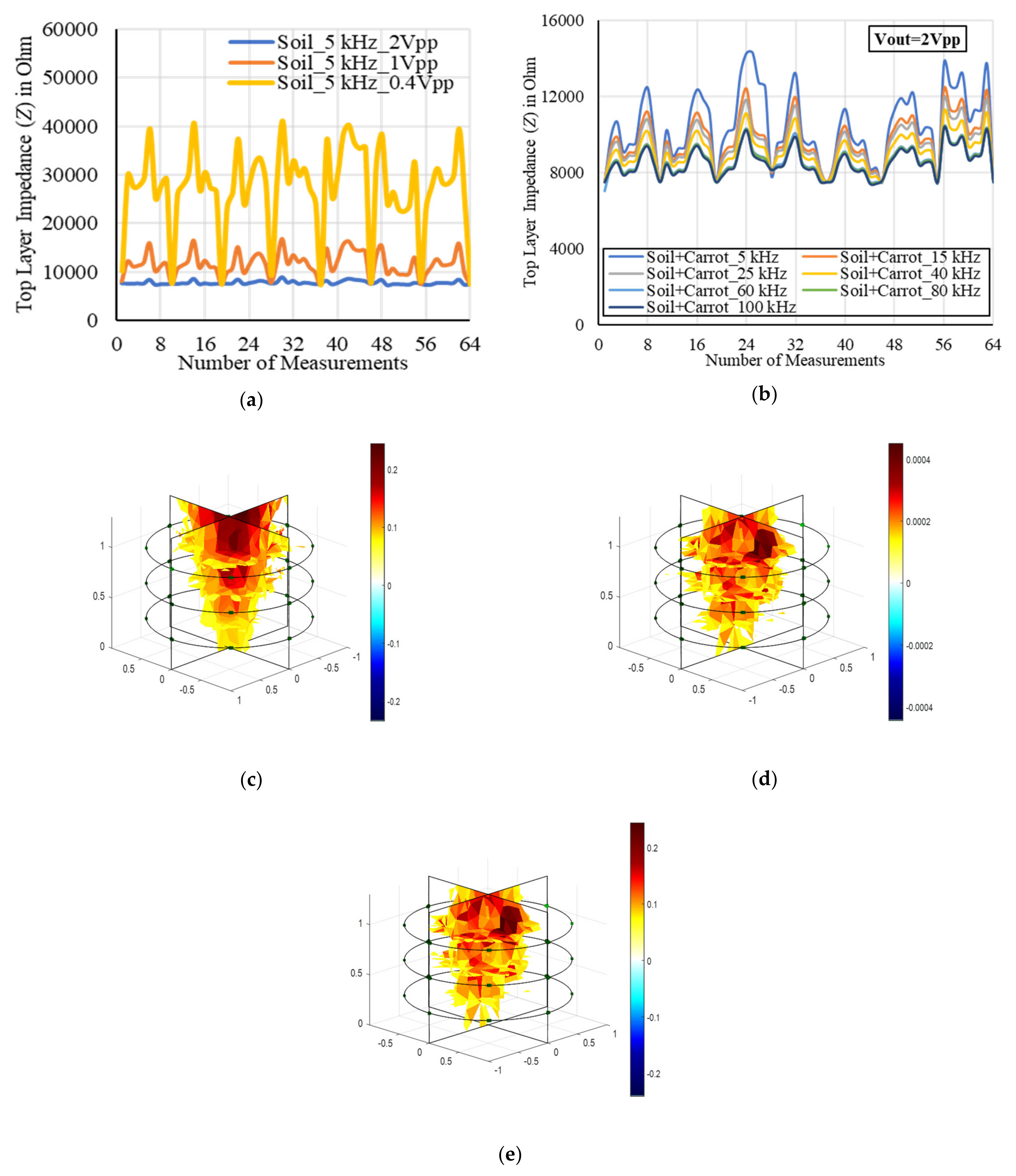
2. Results
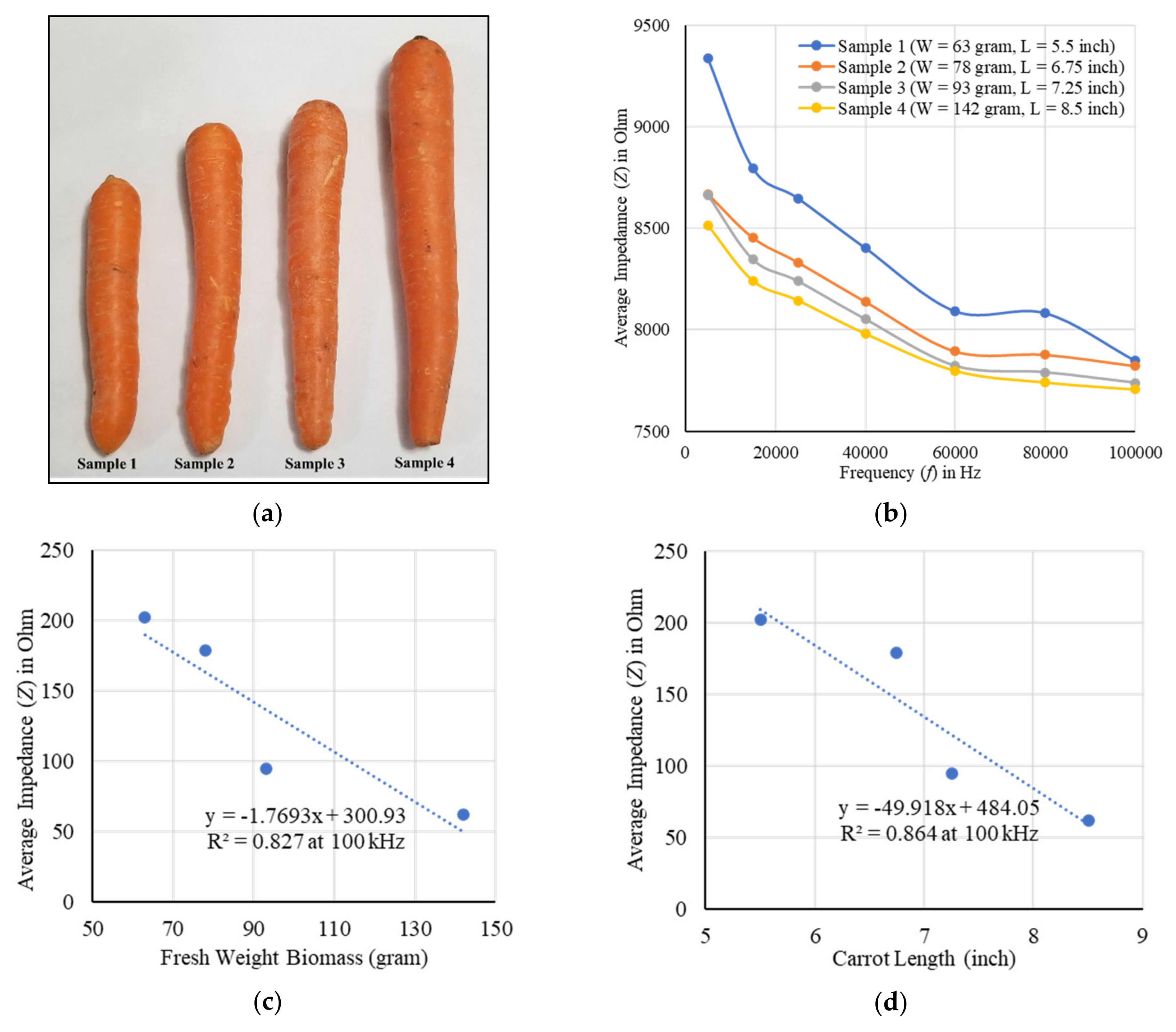
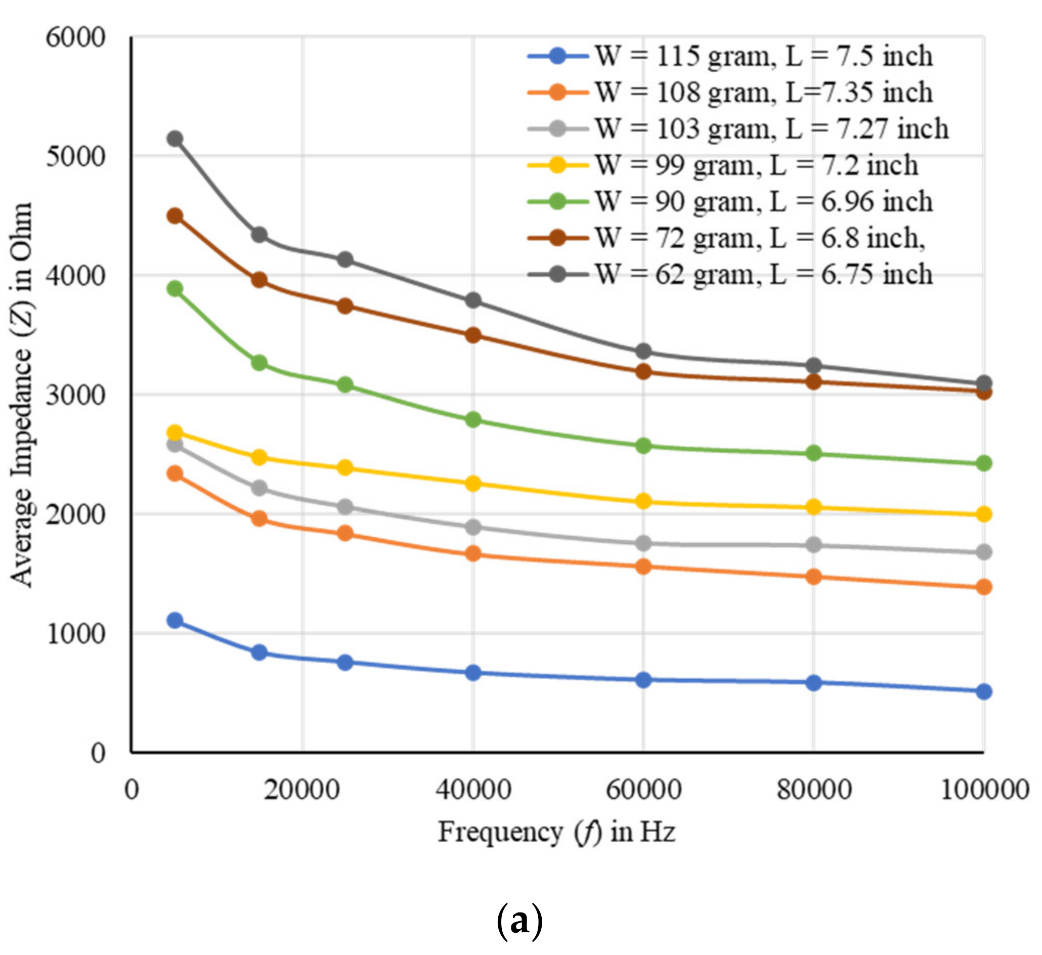
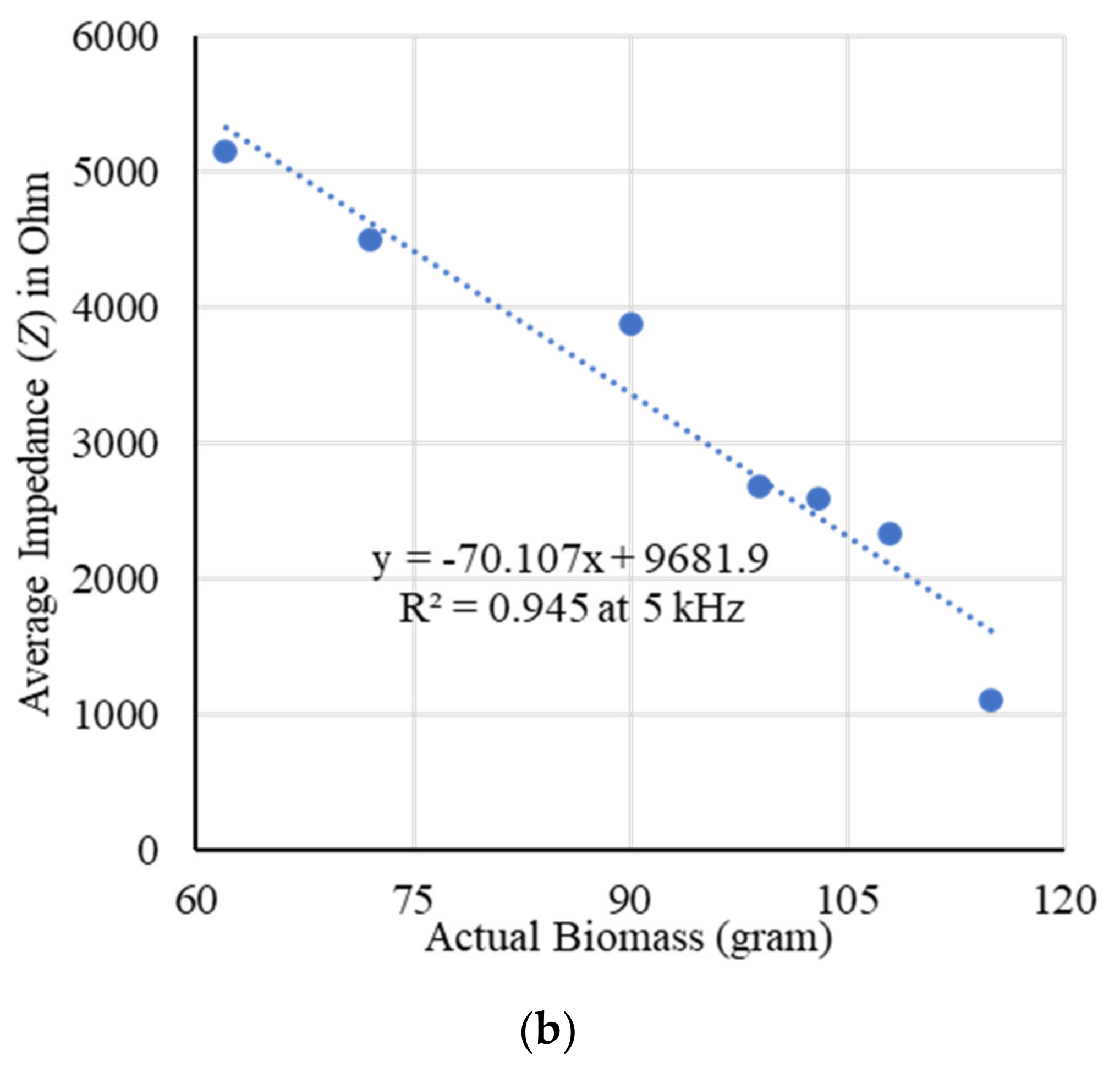
2.1. Fresh Weight Biomass Estimation
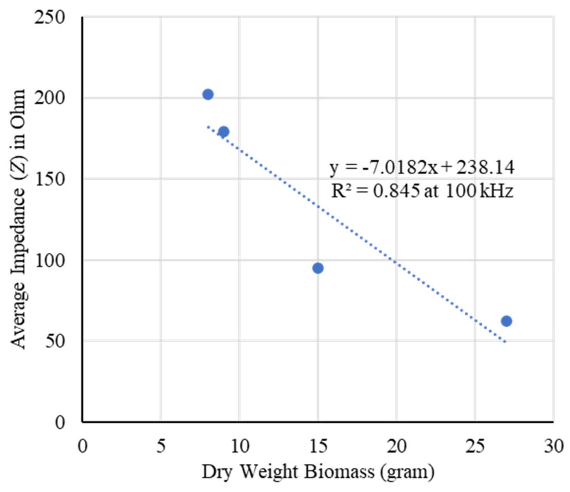
2.2. Dry Weight Biomass Estimation
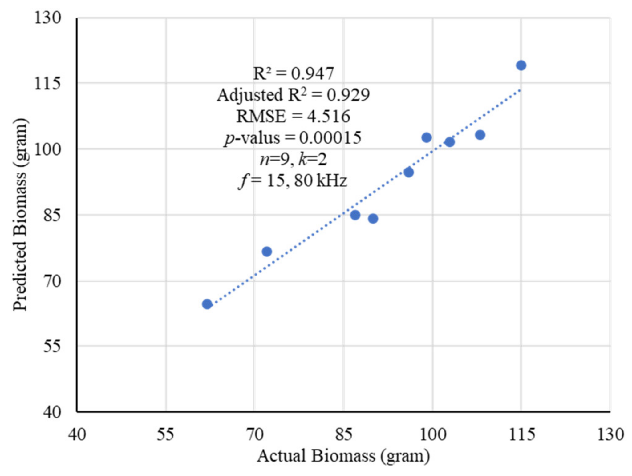
2.3. Modeling and Estimation of Actual Biomass Weight
3. Discussion
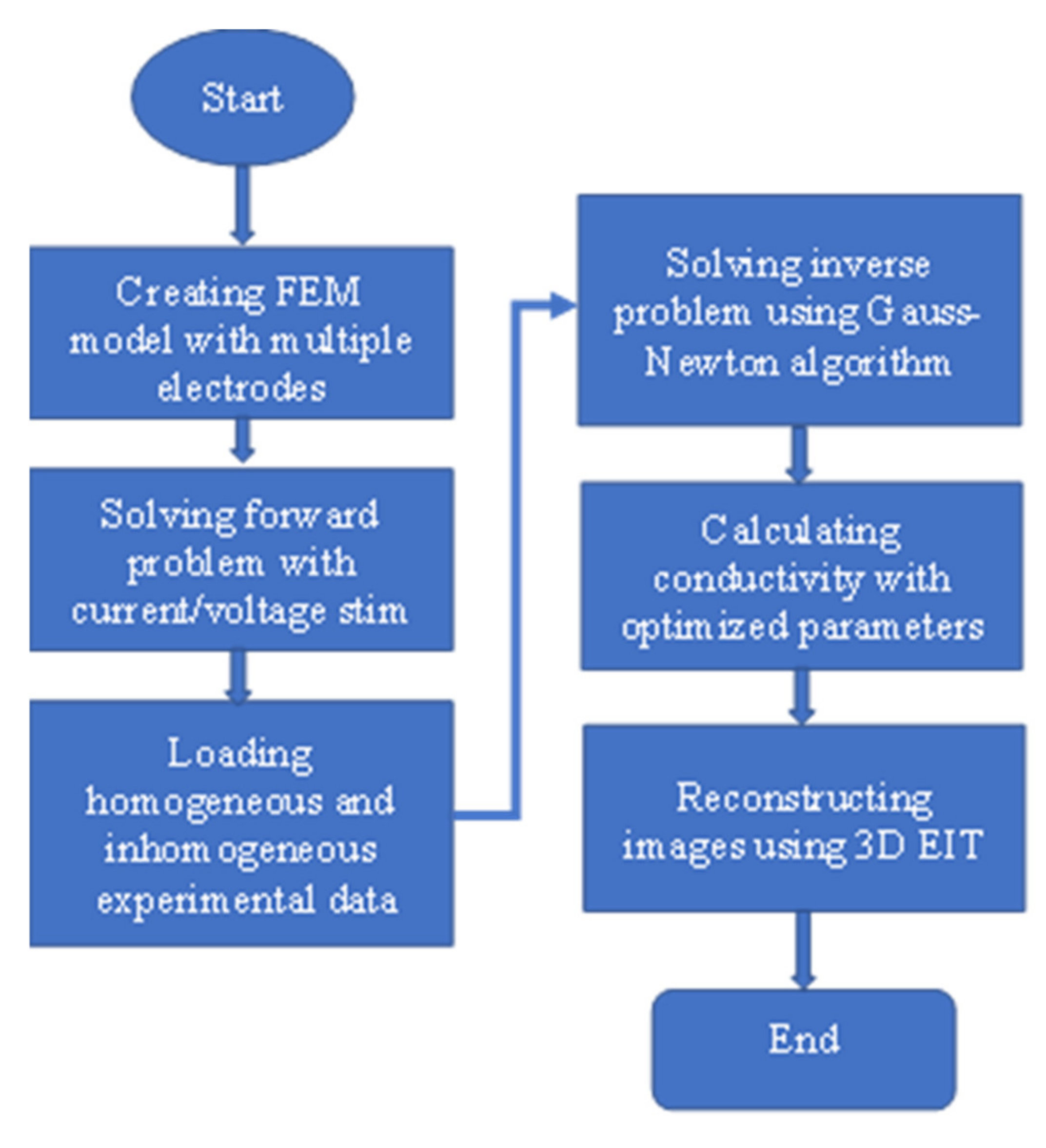
4. Materials and Methods
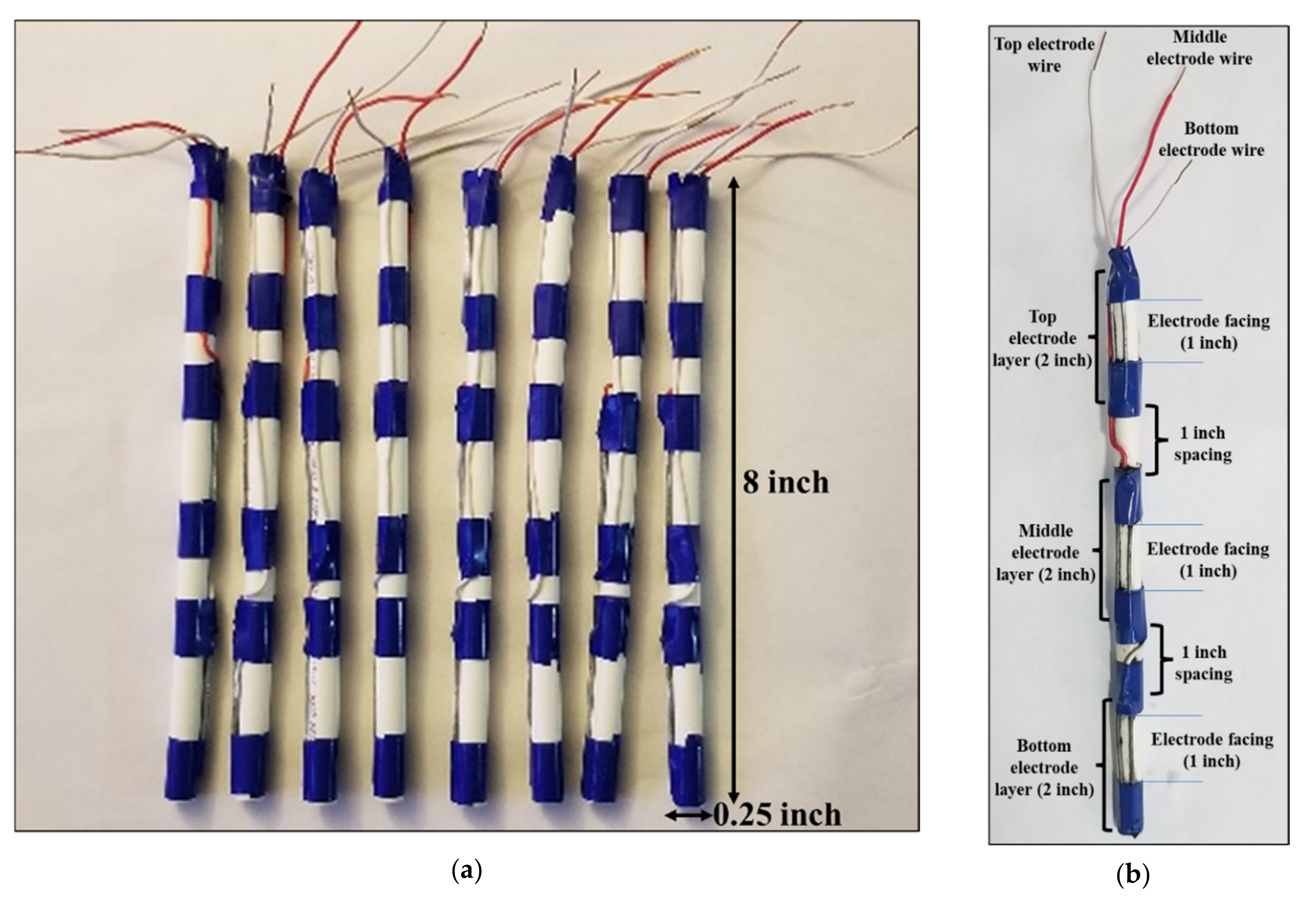
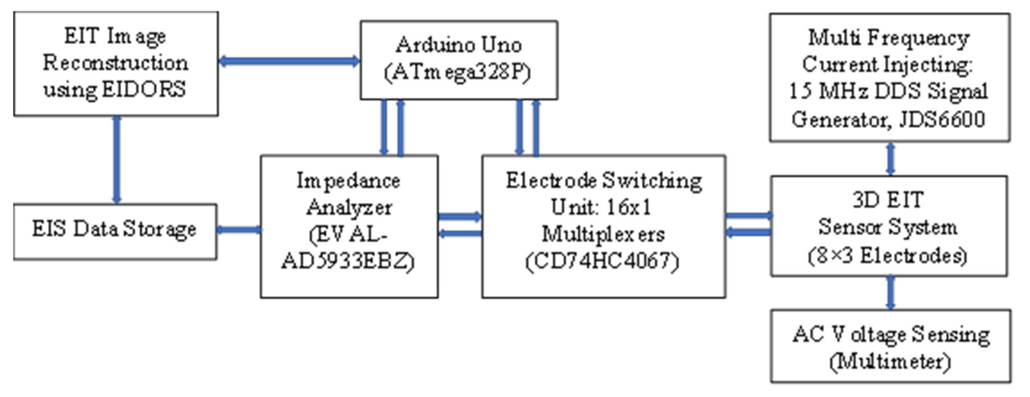
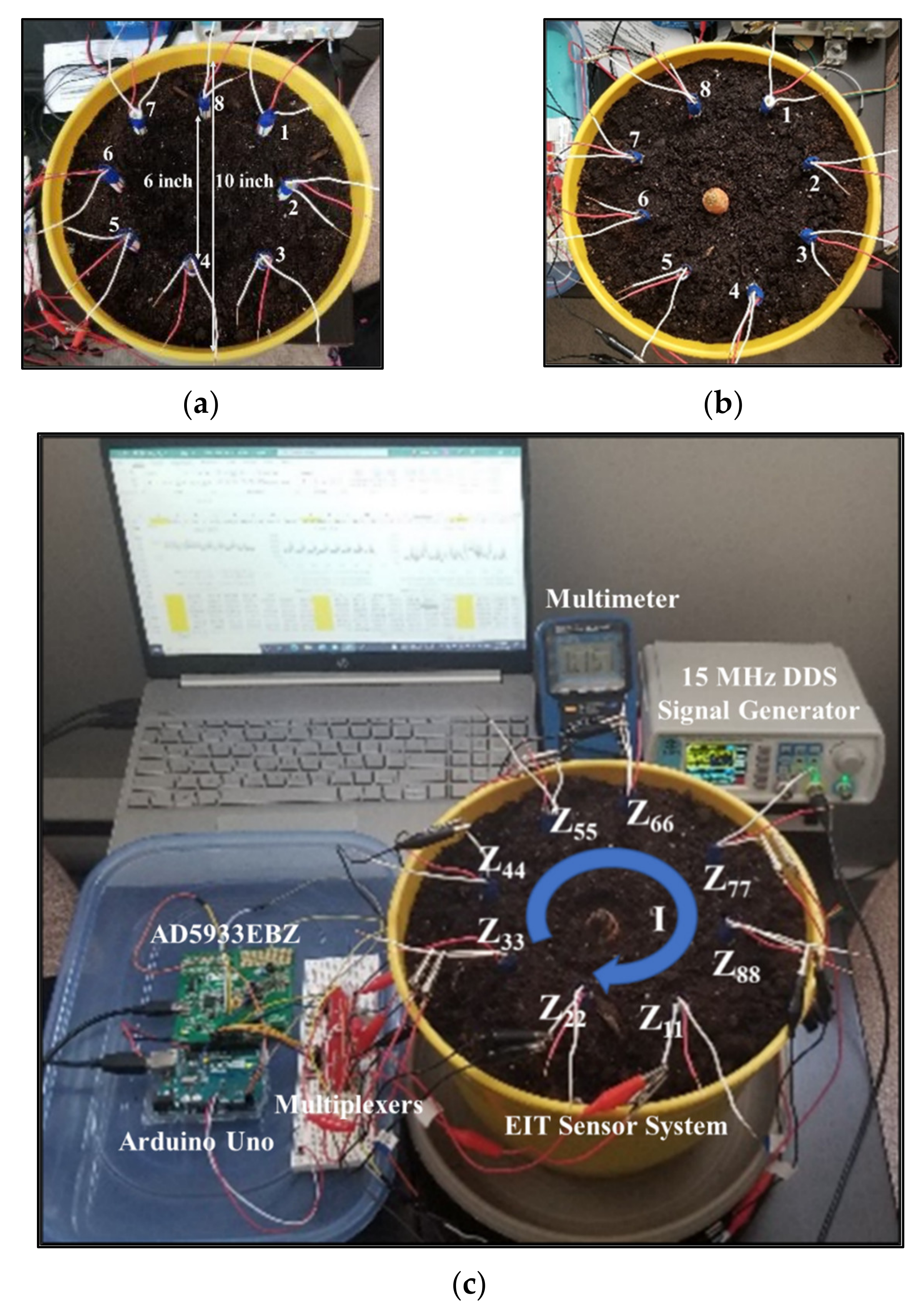
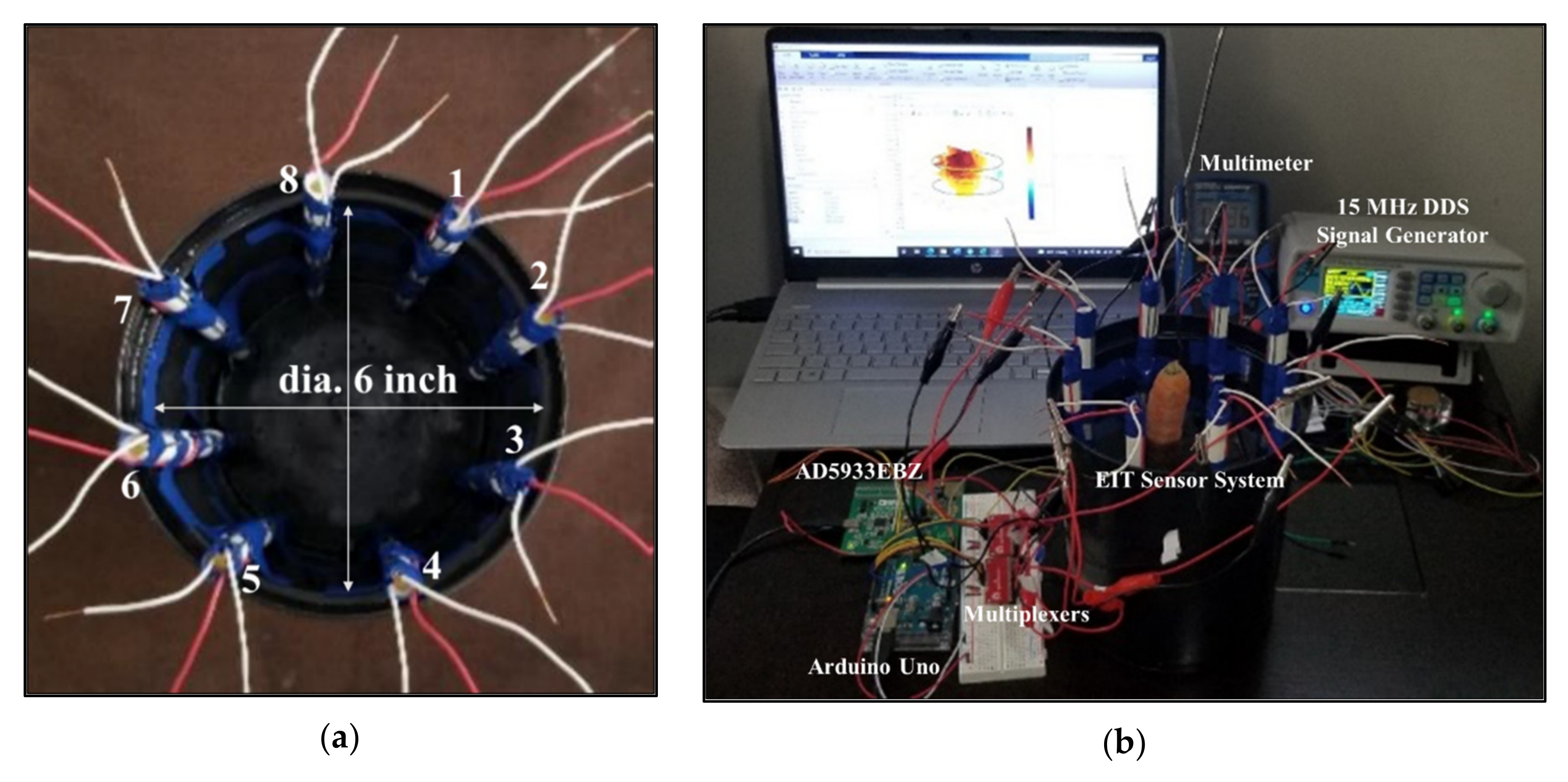
4.1. Design of EIT Sensor System
4.2. Development of EIT Data Acquisition System
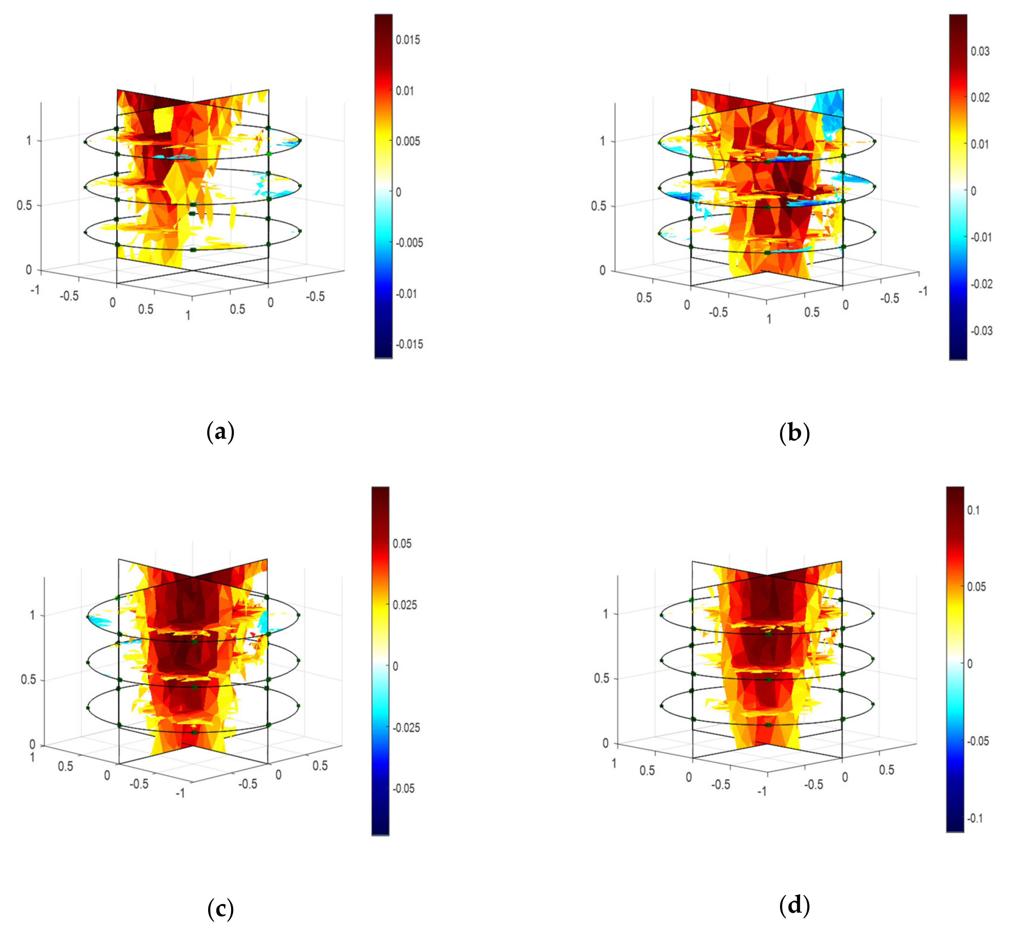
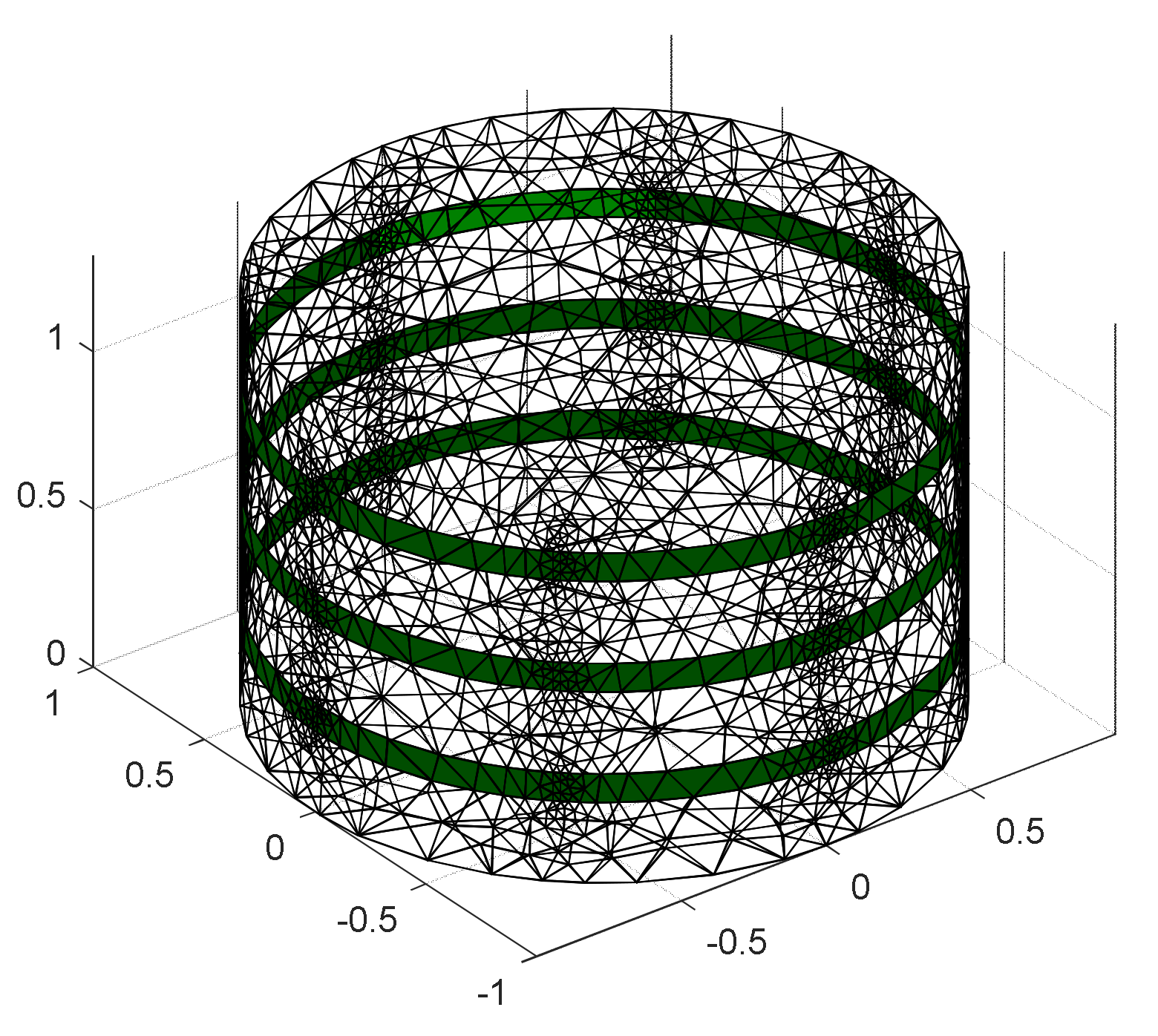
4.3. Modeling and Calculating Conductivity
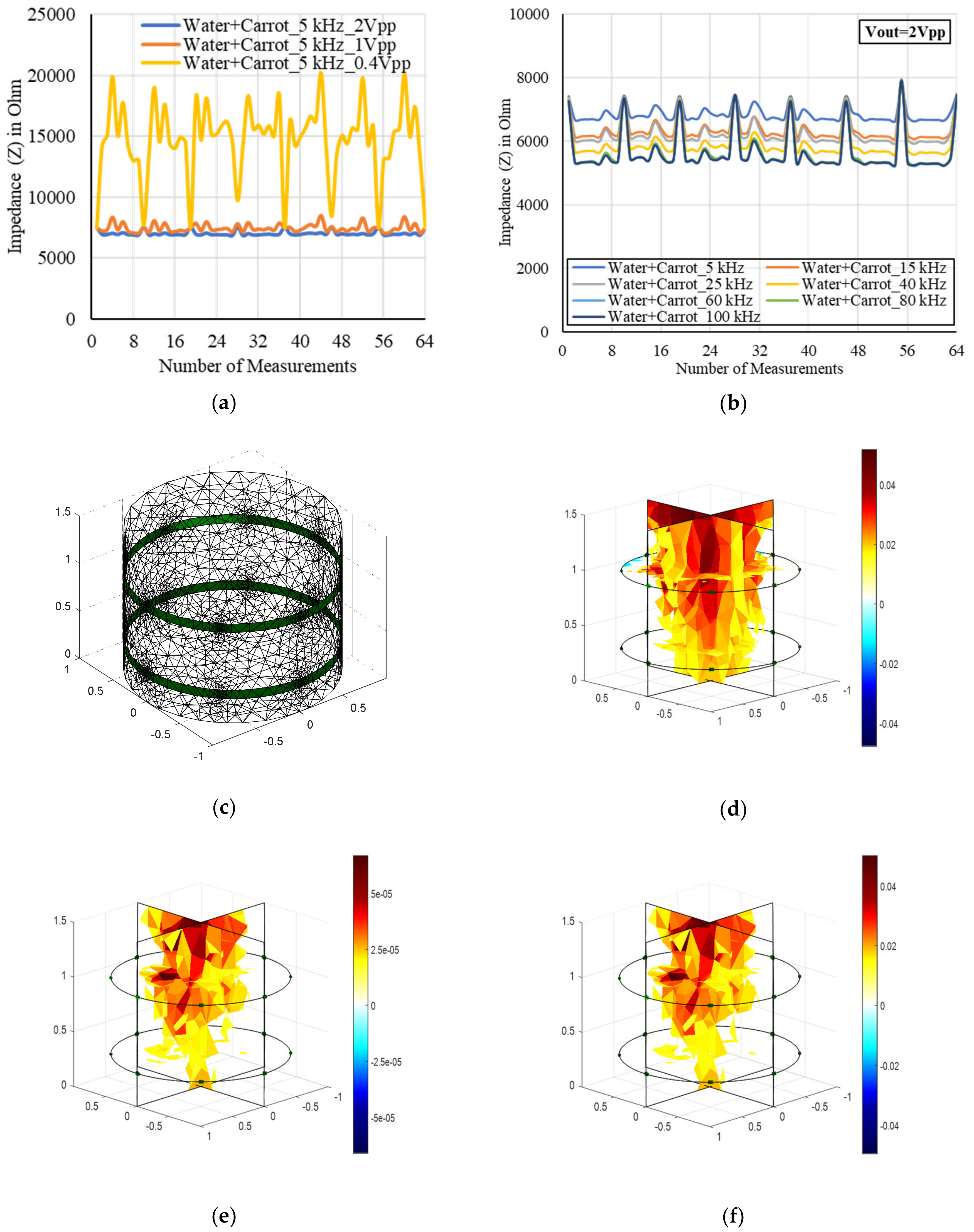
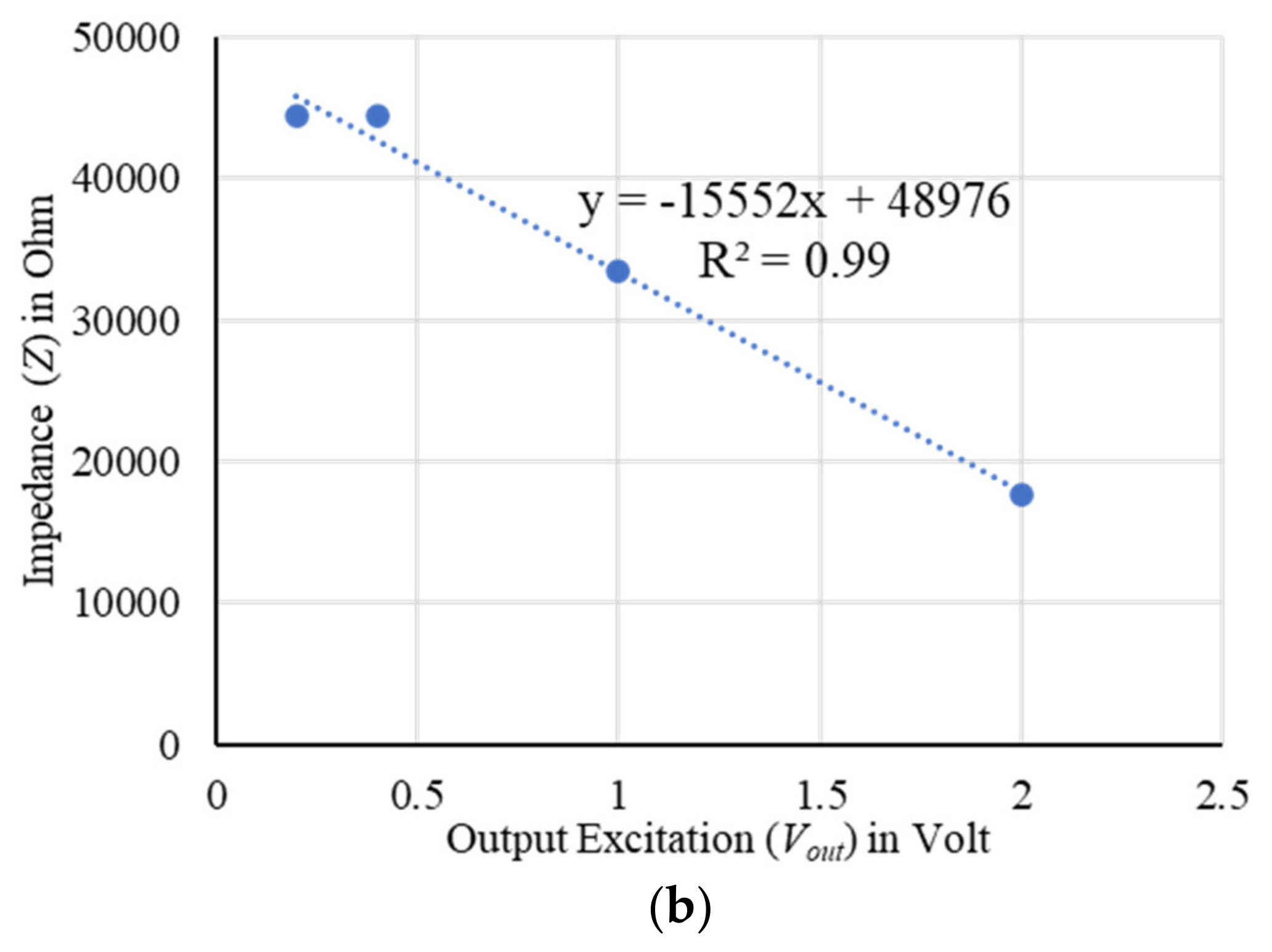
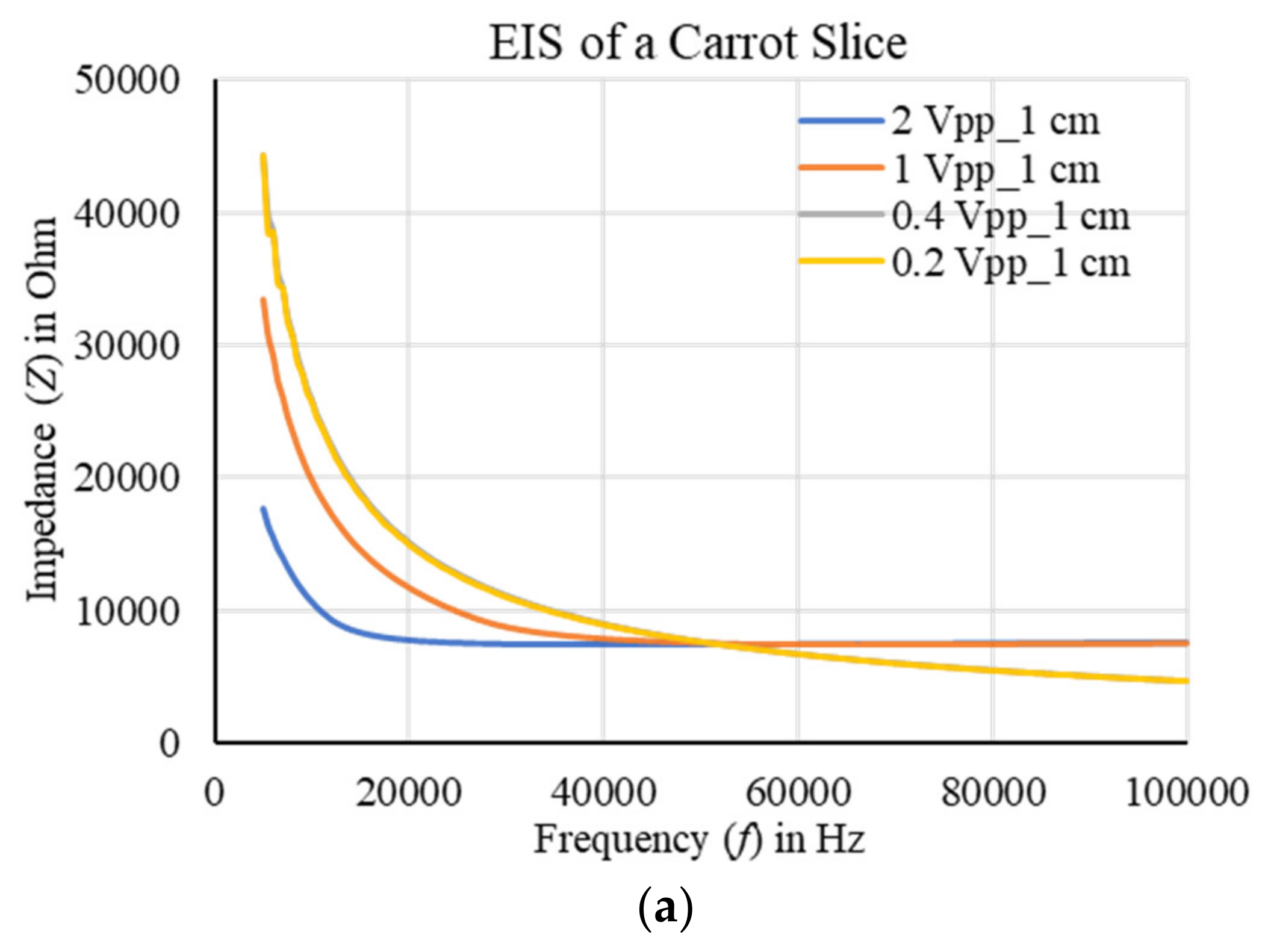
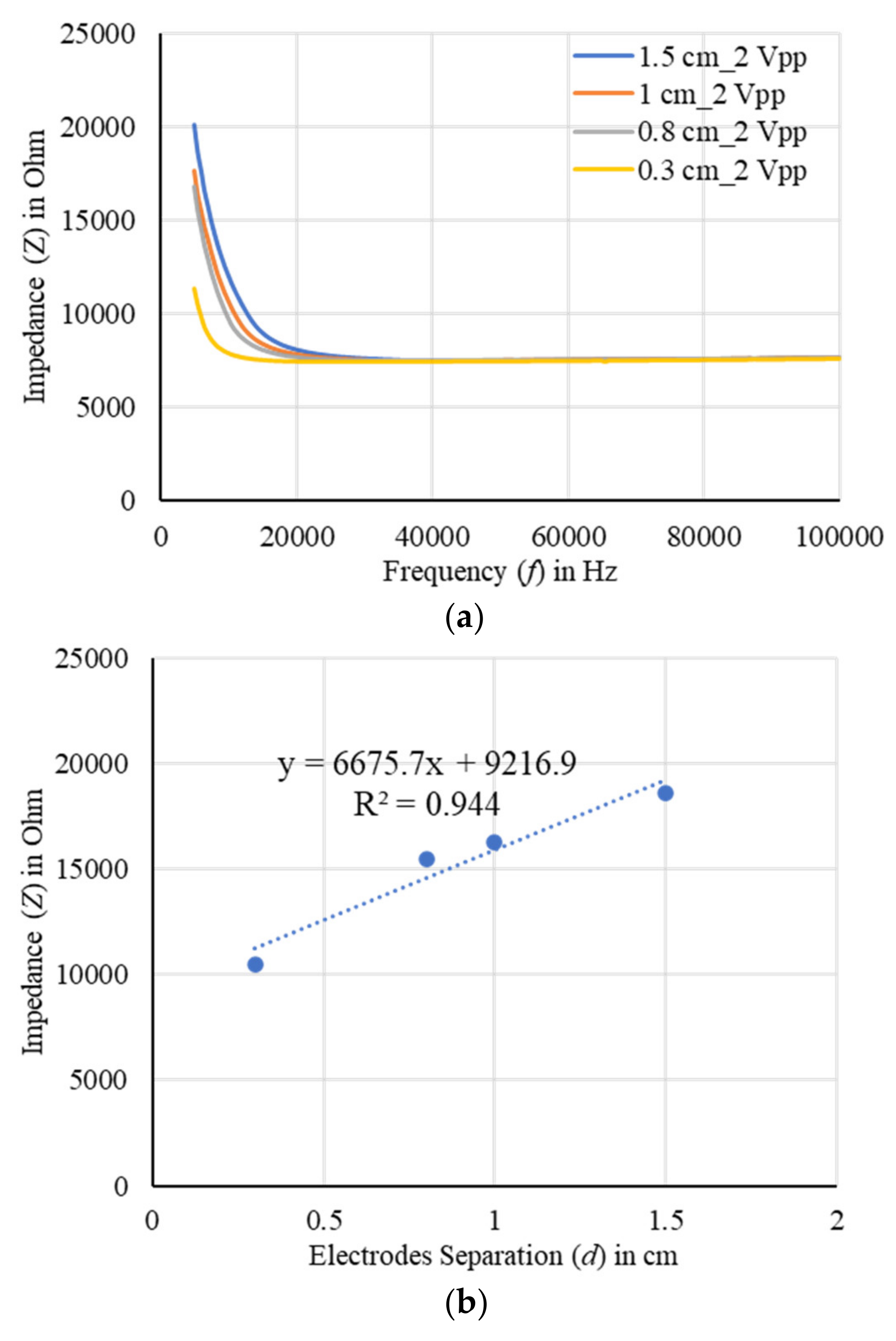
4.4. Sensor Characterization
4.5. Data Process and Analysis
5. Conclusions
Author Contributions
Funding
Data Availability Statement
Acknowledgments
Conflicts of Interest
References
- Wang, H.; Liu, K.; Wu, Y.; Wang, S.; Zhang, Z.; Li, F.; Yao, J. Image Reconstruction for Electrical Impedance Tomography Using Radial Basis Function Neural Network Based on Hybrid Particle Swarm Optimization Algorithm. IEEE Sens. J. 2021, 21, 1926–1934. [Google Scholar] [CrossRef]
- Kim, B.S.; Khambampati, A.K.; Jang, Y.J.; Kim, K.Y.; Kim, S. Image reconstruction using voltage–current system in electrical impedance tomography. Nucl. Eng. Des. 2014, 278, 134–140. [Google Scholar] [CrossRef]
- Bera, T.K.; Nagaraju, J. A MATLAB-Based Boundary Data Simulator for Studying the Resistivity Reconstruction Using Neighbouring Current Pattern. J. Med. Eng. 2013, 2013, 193578. [Google Scholar] [CrossRef] [PubMed] [Green Version]
- Malone, E.; dos Santos, G.S.; Holder, D.; Arridge, S. Multifrequency Electrical Impedance Tomography Using Spectral Constraints. IEEE Trans. Med. Imaging 2014, 33, 340–350. [Google Scholar] [CrossRef]
- Bera, T.K.; Nagaraju, J.; Lubineau, G. Electrical impedance spectroscopy (EIS)-based evaluation of biological tissue phantoms to study multifrequency electrical impedance tomography (Mf-EIT) systems. J. Vis. 2016, 19, 691–713. [Google Scholar] [CrossRef]
- Malone, E.; dos Santos, G.S.; Holder, D.; Arridge, S. A Reconstruction-Classification Method for Multifrequency Electrical Impedance Tomography. IEEE Trans. Med. Imaging 2015, 34, 1486–1497. [Google Scholar] [CrossRef]
- Liu, S.; Huang, Y.; Wu, H.; Tan, C.; Jia, J. Efficient Multi-Task Structure-Aware Sparse Bayesian Learning for Frequency-Difference Electrical Impedance Tomography. IEEE Trans. Ind. Inform. 2021, 17, 463–472. [Google Scholar] [CrossRef] [Green Version]
- Russo, S.; Nefti-Meziani, S.; Carbonaro, N.; Tognetti, A. A Quantitative Evaluation of Drive Pattern Selection for Optimizing EIT-Based Stretchable Sensors. Sensors 2017, 17, 1999. [Google Scholar] [CrossRef]
- Loyola, B.R.; Saponara, V.L.; Loh, K.J.; Briggs, T.M.; O’Bryan, G.; Skinner, J.L. Spatial Sensing Using Electrical Impedance Tomography. IEEE Sens. J. 2013, 13, 2357–2367. [Google Scholar] [CrossRef]
- Weigand, M.; Kemna, A. Multi-frequency electrical impedance tomography as a non-invasive tool to characterize and monitor crop root systems. Biogeosciences 2017, 14, 921–939. [Google Scholar] [CrossRef] [Green Version]
- Weigand, M.; Kemna, A. Imaging and functional characterization of crop root systems using spectroscopic electrical impedance measurements. Plant Soil 2019, 435, 201–224. [Google Scholar] [CrossRef] [Green Version]
- Corona-Lopez, D.D.J.; Sommer, S.; Rolfe, S.A.; Podd, F.; Grieve, B.D. Electrical impedance tomography as a tool for phenotyping plant roots. Plant Methods 2019, 15, 49. [Google Scholar] [CrossRef] [PubMed] [Green Version]
- Zamora-Arellano, F.; López-Bonilla, O.R.; García-Guerrero, E.E.; Olguín-Tiznado, J.E.; Inzunza-González, E.; López-Mancilla, D.; Tlelo-Cuautle, E. Development of a Portable, Reliable and Low-Cost Electrical Impedance Tomography System Using an Embedded System. Electronics 2021, 10, 15. [Google Scholar] [CrossRef]
- Aris, W. Endarko. Design of low-cost and high-speed portable two-dimensional electrical impedance tomography (EIT). Int. J. Eng. Technol. 2018, 7, 6458–6463. [Google Scholar]
- Singh, G.; Anand, S.; Lall, B.; Srivastava, A.; Singh, V. A Low-Cost Portable Wireless Multi-frequency Electrical Impedance Tomography System. Arab. J. Sci. Eng. 2019, 44, 2305–2320. [Google Scholar] [CrossRef]
- Liu, S.; Jia, J.; Zhang, Y.D.; Yang, Y. Image Reconstruction in Electrical Impedance Tomography Based on Structure-Aware Sparse Bayesian Learning. IEEE Trans. Med. Imaging 2018, 37, 2090–2102. [Google Scholar] [CrossRef] [Green Version]
- Liu, D.; Khambampati, A.K.; Du, J. A Parametric Level Set Method for Electrical Impedance Tomography. IEEE Trans. Med. Imaging 2018, 37, 451–460. [Google Scholar] [CrossRef]
- Yang, Y.; Jia, J. An Image Reconstruction Algorithm for Electrical Impedance Tomography Using Adaptive Group Sparsity Constraint. IEEE Trans. Inst. Meas. 2017, 66, 2295–2305. [Google Scholar] [CrossRef] [Green Version]
- Ren, S.; Wang, Y.; Liang, G.; Dong, F. A Robust Inclusion Boundary Reconstructor for Electrical Impedance Tomography with Geometric Constraints. IEEE Trans. Instrum. Meas. 2019, 68, 762–773. [Google Scholar] [CrossRef]
- Shi, X.; Li, W.; You, F.; Huo, X.; Xu, C.; Ji, Z.; Liu, R.; Liu, B.; Li, Y.; Fu, F.; et al. High-Precision Electrical Impedance Tomography Data Acquisition System for Brain Imaging. IEEE Sens. J. 2018, 18, 5974–5984. [Google Scholar] [CrossRef]
- Sapuan, I.; Yasin, M.; Ain, K.; Apsari, R. Anomaly Detection Using Electric Impedance Tomography Based on Real and Imaginary Images. Sensors 2020, 20, 1907. [Google Scholar] [CrossRef] [PubMed] [Green Version]
- Bai, X.; Liu, D.; Wei, J.; Bai, X.; Sun, S.; Tian, W. Simultaneous Imaging of Bio- and Non-Conductive Targets by Combining Frequency and Time Difference Imaging Methods in Electrical Impedance Tomography. Biosensors 2021, 11, 176. [Google Scholar] [CrossRef] [PubMed]
- Yang, Y.; Jia, J.; Smith, S.; Jamil, N.; Gamal, W.; Bagnaninchi, P. A Miniature Electrical Impedance Tomography Sensor and 3D Image Reconstruction for Cell Imaging. IEEE Sens. J. 2017, 17, 514–523. [Google Scholar] [CrossRef] [Green Version]
- Ozier-Lafontaine, H.; Bajazet, T. Analysis of root growth by impedance spectroscopy (EIS). Plant Soil 2005, 277, 299–313. [Google Scholar] [CrossRef]
- Liao, A.; Zhou, Q.; Zhang, Y. Application of 3D electrical capacitance tomography in probing anomalous blocks in water. J. Appl. Geophys. 2015, 117, 91–103. [Google Scholar] [CrossRef]
- Postic, F.; Doussan, C. Benchmarking electrical methods for rapid estimation of root biomass. Plant Methods 2016, 12, 33. [Google Scholar] [CrossRef] [Green Version]
- Newill, P.; Karadaglic, D.; Podd, F.; Grieve, B.D.; York, T.A. Electrical impedance imaging of water distribution in the root zone. Meas. Sci. Technol. 2014, 25, 055110. [Google Scholar] [CrossRef] [Green Version]
- Tan, C.; Liu, S.; Jia, J.; Dong, F. A Wideband Electrical Impedance Tomography System based on Sensitive Bioimpedance Spectrum Bandwidth. IEEE Trans. Instrum. Meas. 2020, 69, 144–154. [Google Scholar] [CrossRef]
- Putensen, C.; Hentze, B.; Muenster, S.; Muders, T. Electrical Impedance Tomography for Cardio-Pulmonary Monitoring. J. Clin. Med. 2019, 8, 1176. [Google Scholar] [CrossRef] [Green Version]
- Rymarczyk, T.; Kłosowski, G.; Kozłowski, E.; Tchórzewski, P. Comparison of Selected Machine Learning Algorithms for Industrial Electrical Tomography. Sensors 2019, 19, 1521. [Google Scholar] [CrossRef] [Green Version]
- Fernández-Fuentes, X.; Mera, D.; Gómez, A.; Vidal-Franco, I. Towards a Fast and Accurate EIT Inverse Problem Solver: A Machine Learning Approach. Electronics 2018, 7, 422. [Google Scholar] [CrossRef] [Green Version]
- Kłosowski, G.; Rymarczyk, T.; Niderla, K.; Rzemieniak, M.; Dmowski, A.; Maj, M. Comparison of Machine Learning Methods for Image Reconstruction Using the LSTM Classifier in Industrial Electrical Tomography. Energies 2021, 14, 7269. [Google Scholar] [CrossRef]
- Chowdhury, R.I.; Basak, R.; Wahid, K.A.; Nugent, K.; Baulch, H. A Rapid Approach to Measure Extracted Chlorophyll-a from Lettuce Leaves using Electrical Impedance Spectroscopy. Water Air Soil Pollut. 2021, 232, 73. [Google Scholar] [CrossRef]
- Graham, B.M.; Adler, A. Electrode placement configurations for 3D EIT. Physiol. Meas. 2007, 28, 29–44. [Google Scholar] [CrossRef] [PubMed]
- Matsiev, L. Improving Performance and Versatility of Systems Based on Single-Frequency DFT Detectors Such as AD5933. Electronics 2015, 4, 1–34. [Google Scholar] [CrossRef] [Green Version]
- Basak, R.; Wahid, K.A.; Dinh, A. Estimation of the Chlorophyll-A Concentration of Algae Species Using Electrical Impedance Spectroscopy. Water 2021, 13, 1223. [Google Scholar] [CrossRef]


| Features | R2 | Adj. R2 | RMSE | p-Value |
|---|---|---|---|---|
| 5 kHz | 0.994 | 0.976 | 2.58 | 0.017 |
| 15 kHz | 0.986 | 0.945 | 3.94 | 0.04 |
| 25 kHz | 0.987 | 0.949 | 3.81 | 0.037 |
| 40 kHz | 0.99 | 0.963 | 3.26 | 0.027 |
| 60 kHz | 0.988 | 0.951 | 3.72 | 0.035 |
| 80 kHz | 0.988 | 0.954 | 3.61 | 0.033 |
| 100 kHz | 0.989 | 0.959 | 3.43 | 0.03 |
| New Carrot Samples | Actual Biomass Weight (g) | Predicted Biomass Weight (g) | Absolute Error (%) |
|---|---|---|---|
| Sample 1 | 142 | 132.034 | 7.01 |
| Sample 2 | 115 | 119.217 | 3.66 |
| Sample 3 | 99 | 102.587 | 3.62 |
| Sample 4 | 96 | 94.67 | 1.38 |
| Sample 5 | 90 | 84.17 | 6.47 |
| Sample 6 | 87 | 84.9 | 2.41 |
| Sample 7 | 62 | 64.68 | 4.32 |
| Weigand and Kemna [10,11] | Corona-Lopez et al. [12] | Proposed EIT Sensor (This Work) | |
|---|---|---|---|
| Sensor design media | Water-filled container | Compost-filled container | Water- and soil-filled container |
| Type and size of electrode array | Static with 38 electrodes | Static with 32 electrodes | Dynamic and adjustable with 24 electrodes |
| Operating frequency (kHz) | 0.00046–45 | 5–10 | 1–100 |
| Imaging capability | Two-dimensional | Three-dimensional | Three-dimensional |
| Measurement sensitivity | Characterize and monitor the tap roots (oilseed) | Visualize the development of tap roots (oilseed) | Evaluate the growth and estimate the biomass of tap roots (carrot) |
Publisher’s Note: MDPI stays neutral with regard to jurisdictional claims in published maps and institutional affiliations. |
© 2022 by the authors. Licensee MDPI, Basel, Switzerland. This article is an open access article distributed under the terms and conditions of the Creative Commons Attribution (CC BY) license (https://creativecommons.org/licenses/by/4.0/).
Share and Cite
Basak, R.; Wahid, K.A. An In Situ Electrical Impedance Tomography Sensor System for Biomass Estimation of Tap Roots. Plants 2022, 11, 1713. https://doi.org/10.3390/plants11131713
Basak R, Wahid KA. An In Situ Electrical Impedance Tomography Sensor System for Biomass Estimation of Tap Roots. Plants. 2022; 11(13):1713. https://doi.org/10.3390/plants11131713
Chicago/Turabian StyleBasak, Rinku, and Khan A. Wahid. 2022. "An In Situ Electrical Impedance Tomography Sensor System for Biomass Estimation of Tap Roots" Plants 11, no. 13: 1713. https://doi.org/10.3390/plants11131713
APA StyleBasak, R., & Wahid, K. A. (2022). An In Situ Electrical Impedance Tomography Sensor System for Biomass Estimation of Tap Roots. Plants, 11(13), 1713. https://doi.org/10.3390/plants11131713