1. Introduction
In recent years, the expansion of the range, transportation mass, types of activities undertaken by human beings has created global environmental problems. Therefore, a transportation system with high-efficiency and low power consumption is one of the important solutions for these problems and will benefit society. For this purpose, in the future, the next-generation transportation system must include two significant features, namely, high speed and high efficiency [
1]. One of the potential candidates is the MAGLEV train which could reach maximum velocity of up to 603 km/h [
2]. However, in spite of the advantages of the technology, the MAGLEV train system has smaller economic efficiency value than that of the Aerotrain [
3], a Wing-in-Ground effect vehicle, proposed by Kohama et al. [
4] at Tohoku University, Japan.
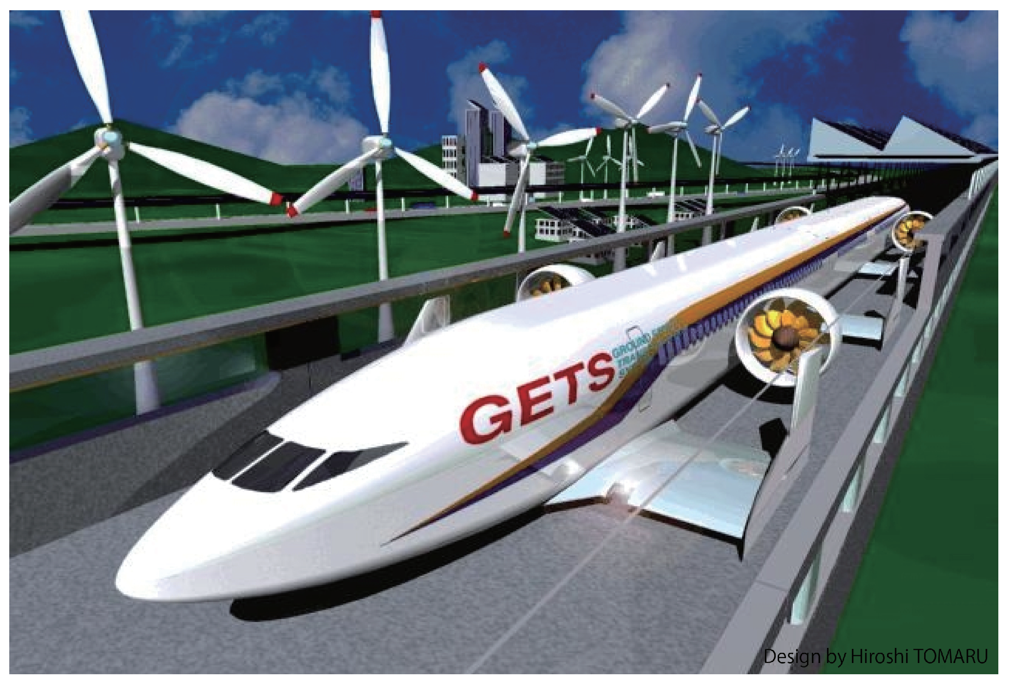
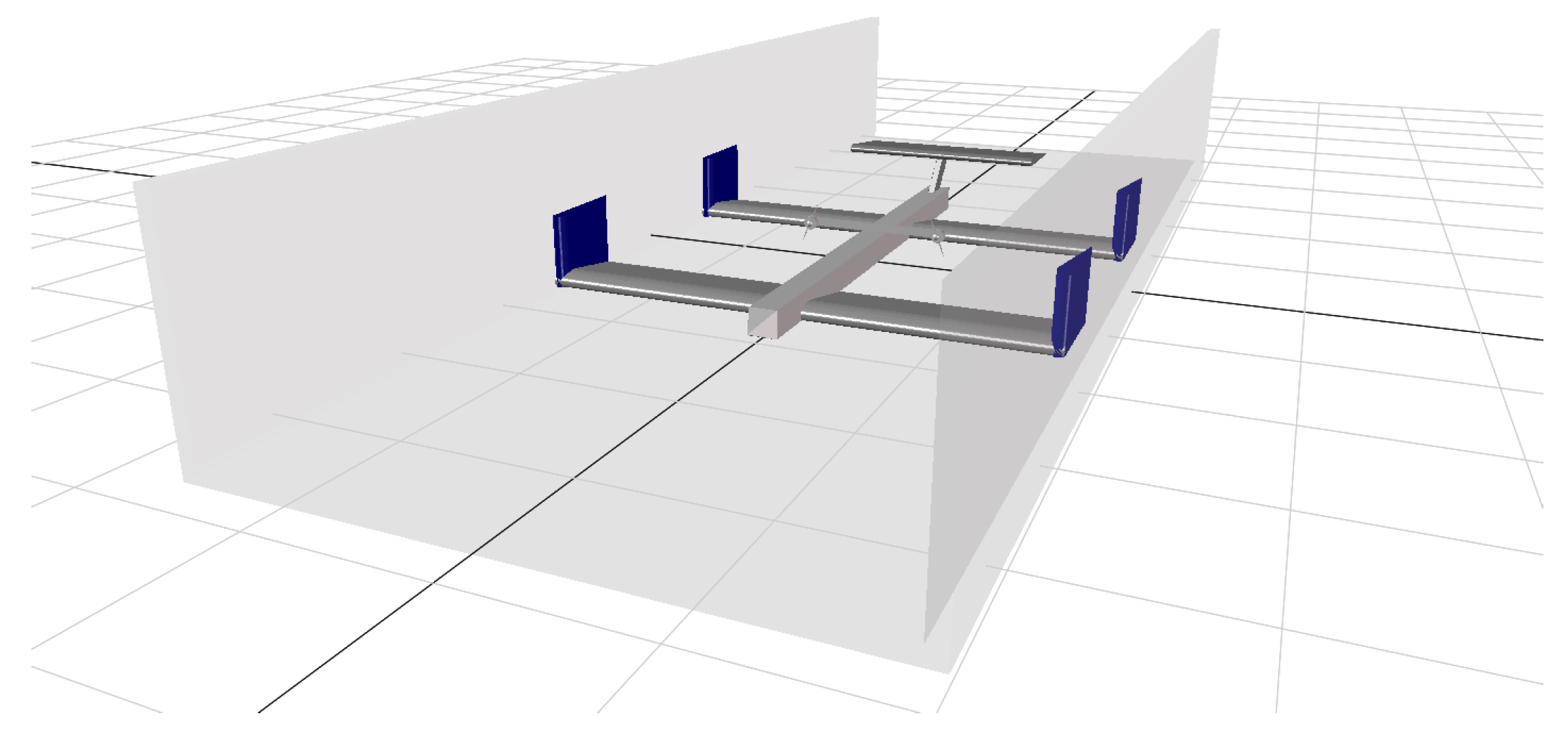
The Aerotrain, as shown in
Figure 1, has wings and levitates on a concrete U-shaped guideway by the Wing-In-Ground (WIG) effect. The advantage of a low-cost guideway is expected to reduce the maintenance cost of the track that up to 30% of the total operation costs according to a High-speed rail feasibility study reported by Rocky Mountain Rail Authority [
5]. Compared with normal MAGLEV high-speed trains, the massive energy required to maintain the electrical magnetic force is not needed, which means that the Aerotrain could reduce a lot of power consumption. The difference between an airplane and the Aerotrain is the WIG effect. The WIG effect happens when an airfoil or wing-like object is close to the ground as shown in
Figure 2 when the altitude h is less than 25% of the wing chord c [
6], a high-pressure air cushion will be created for the stagnation of the air which generates a greater lift force and a greater lift-drag ratio (L/D) than the airfoil at higher altitude. When travelling, the pitching and rolling motion of the vehicle are controlled through the control surfaces on the levitation wings. The aerodynamic lift generated from levitation wings will levitate the train very close to the ground under WIG effect. Thus, a greater lift force under WIG effect benefits the Aerotrain a higher aerodynamic efficiency than that of conventional airplanes. This same principle is adopted to the guide wing for keeping the position of the train at the center of the guideway and keeping the direction parallel to the guideway. By changing the angle of the control surface on the guide wing (the vertical wings at the tip of the levitation wings), the side force and the yawing moment are also changed to make the Aerotrain stay on the proper track. The WIG effect could also provide a recovering moment to ensure the stability of the Aerotrain when an external disturbance in the rolling axis of motion happens.
The development of WIG effect vehicles in general and WIG crafts (operating on water surface) in particular have showed rapidly technical improvement in recent years. Hameed [
8] and Matdaud [
9] have an extensive literature review on the design and the existing stability control system technology’s development and enhancement for WIG crafts. According to the reviews, each WIG craft configuration shows its own main design features, advantages and yet disadvantages. With the presence of the disturbance caused by the round wave condition, stability problems arise that make safety issues of operating WIG crafts become more delicate to handle. Compared with those conventional WIG crafts [
10,
11,
12,
13], the Aerotrain has less external disturbances and it is safer because the operation of the vehicle is based on the use of a solid guideway [
3]. There have been several studies on the control of the Aerotrain [
14,
15,
16], but there is insufficient knowledge on the design of the vehicle body which has a desirable dynamic characteristic. Thus, the design of the Aerotrain with only levitation wings and guide wings is controllable, but does not have dynamic stability. A recent study [
3] found the influence of the relative positions of the levitation wings and the angle of attack on the aerodynamic performances of the Aerotrain. However, in an experiment of the previous research, the prototype could not regain stability as it was pitching the nose up until it became stall when losing its control [
17]. That potential risk raised a question about the relationship between the body design of the vehicle and its stability. Therefore, to answer the question, the long-term objective of this research is to investigate the relationship between the Aerotrain’s design parameters and its stability.
Generally, the longitudinal stability plays an important role in the stability of the vehicle and it could be studied separately with directional and lateral stability. Moreover, as for a flying vehicle which have a symmetrical shape about the centerline, moderate changes in angle of attack will have little or no influence upon the yaw or roll. This permits the stability and control analysis to be divided into longitudinal and lateral-directional analysis [
18]. According to this assumption, the previous study [
19] found that the horizontal tail has a great contribution on the longitudinal stability of the Aerotrain by introducing a two-dimensional dynamic model. The purpose of this paper is to deeply clarify the design-stability relation in a complicated condition when longitudinal, lateral and directional stability are all considered. In this paper, firstly, a three-dimensional nonlinear dynamic model of the Aerotrain with a horizontal tail and a vertical tail has been introduced. Secondly, based on the dynamic model, the effect of the horizontal tail design (horizontal tail location and horizontal tail area), the vertical tail design (vertical tail location and vertical tail area) and levitation wing design (flat levitation wing and dihedral levitation wing) to the dynamic stability of the Aerotrain has been evaluated through several indices that will be explained later in
Section 3.
2. Dynamic Model of the Aerotrain
Considering it as a flight vehicle, the attitude of the Aerotrain is described in a body-fixed coordinate system
in which the origin is the center of gravity of the vehicle. The
X-axis is in the plane of symmetry of the body and points forward. The
Z-axis is in the same plane as
X-axis, perpendicular to
X-axis and points down. The
Y-axis is perpendicular to the symmetry plane and points out the right wing. However, only using the body-fixed coordinate system is not enough to express the gravitational force acting on the vehicle. Thus, the orientation of the body-fixed coordinate system with respect to the gravity vector needs to be determined as shown in
Figure 3. This orientation can be specified using the Euler angle (pitch angle
, roll angle
and yaw angle
) of the body-fixed coordinate system with respect to an inertial system
, where the inertial system is oriented such that the
-axis points down (parallel to the gravity vector), the
-axis points North and the
-axis completes the right-handed system, and therefore points East.
The Aerotrain is considered as a rigid body in steady state with a total of 6 degrees of freedom which include 3 translations and 3 rotation motions. The 3 translations are caused by the aerodynamic forces and the gravity force. These forces and aerodynamic moments are the reason of the 3 rotational motions which are pitching, rolling and yawing moment. In the Aerotrain model, the aerodynamic lifts generated from two levitation wings and 4 guide wings are under the WIG effect during cruise speed. Given that the operation occurs inside a U-shaped guideway, the movement in Z-axis and Y-axis and the rotation about 3 axes are more important than the movement in X-axis. Thus, in this paper, the 1 degree of freedom of the X-axis translation has been ignored under the assumption that the vehicle travels at constant speed. Therefore, Z-axis and Y-axis forces as well as 3 moments (about 3 axes) have been modelled.
2.1. Wing-in-Ground Effect Model
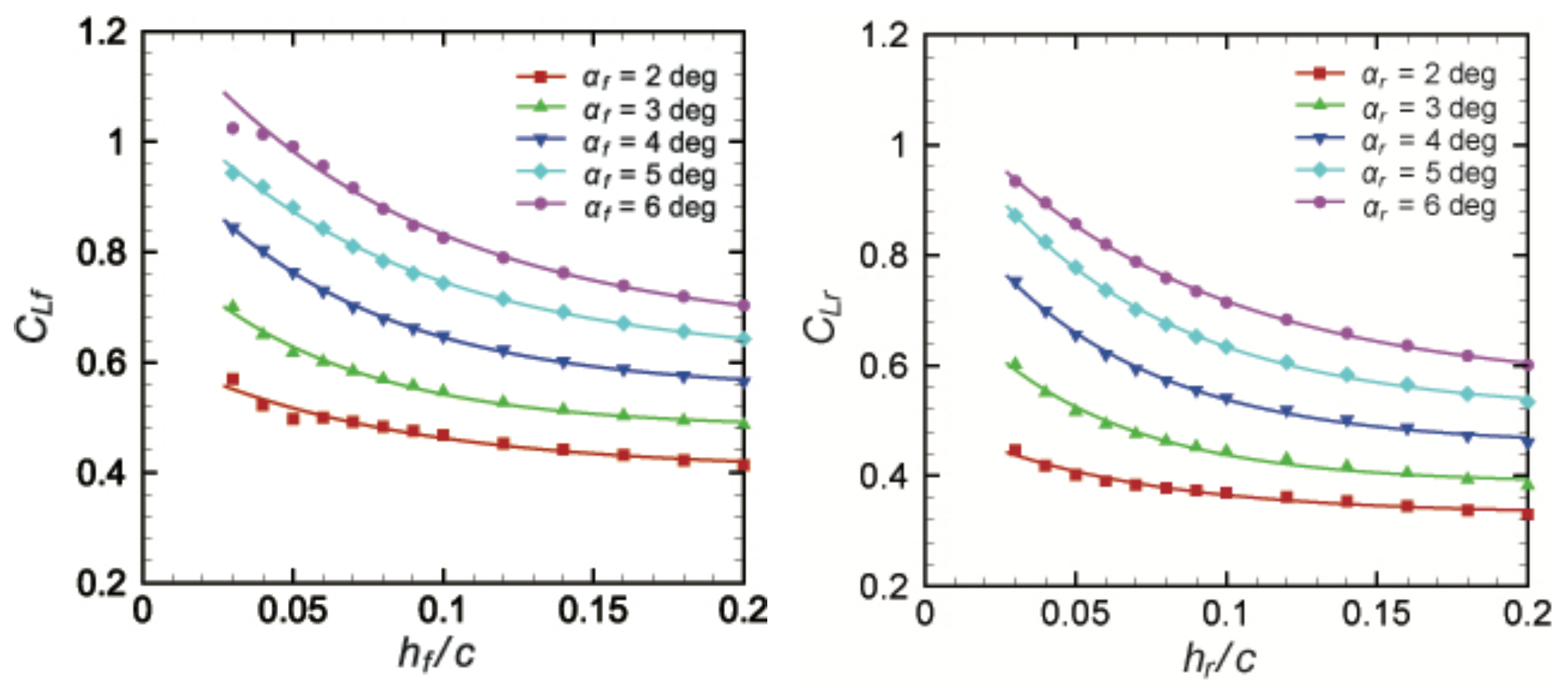
According to Honda [
20], in the area affected by the ground effect, the lift coefficient changes nonlinearly, but this can be represented by the sum of the nonlinear term caused by the influence of the ground effect and the linear term unrelated to the influence of the ground effect.
where
L is the aerodynamic lift,
is the lift coefficient,
is the air density,
is the velocity at steady state and
S is the wing area. The lift coefficient under the WIG effect
and in normal condition
could be expressed as followings:
where
are obtained constants from the curve fitting of the experimental results, and they are different at the front and rear levitation wings as can be seen in
Figure 4;
is the angle of attack. In
Figure 4,
are the aerodynamic lift coefficient of the front and rear levitation wings;
are the height of the front and rear levitation wings;
are the angle of attack of the front and rear levitation wings.
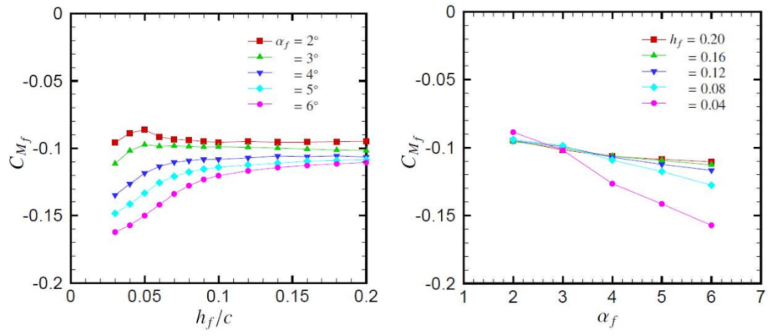
Similar to the aerodynamic lift, the aerodynamic moment under WIG effect is nonlinear, and it can be represented by the sum of the nonlinear term caused by the WIG effect and the linear term unrelated to the influence of the WIG effect.
where
m is the aerodynamic moment,
is the moment coefficient. The moment coefficient under WIG effect
and in normal condition
could be expressed as followings:
where
are obtained constants from the curve fitting of the experimental results as can be seen in
Figure 5, and they are also different at the front and rear levitation wings [
20].
in the
Figure 5 is the aerodynamic coefficient of the front levitation wing.
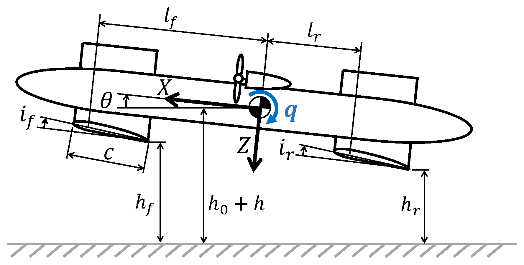
2.2. Aerodynamic Force along the Z-Axis
The aerodynamic force along the
Z-axis includes the lift force from the front and the rear levitation wing of the Aerotrain.
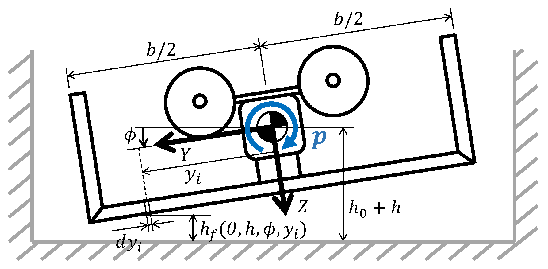
Figure 6 shows the differential slice
with its height
at the spanwise
of the front levitation wing with span
b at the roll angle
that will be later used to calculate the differential lift.
is the height of the Center of Gravity (CoG) of Aerotrain at the steady state, and
h is the displacement of the CoG from the steady state in the
Z-axis.
Under the influence of the WIG effect, the lift coefficient of the front wing
and the rear wing
at the spanwise
could be written as:
The parameters
are defined by the curve fitting from the experiment [
20];
are the chord length of the front and rear levitation wing relatively. Assume that the pitch angle
and roll angle
are small enough, from the geometrical relationship shown in
Figure 7, the height of the front wing
and the rear wing
are the linearized function of the actual height
h of the CoG, the pitch angle
, the roll angle
and the location
:
where
are the distance from the CoG to the aerodynamic center which is located at the quarter-chord from the leading edge of the front and the rear levitation wing as shown in
Figure 7.
The Angle of Attack (AOA) of the front wing
and the rear wing
are the function of the AOA
and the pitching angular velocity
q:
where
are the mounting angle. By integrating along the wing span, the total aerodynamic force
along the
Z-axis can be obtained from the sum of the aerodynamic lift
of the front and rear levitation wing.
2.3. Aerodynamic Force along the Y-Axis
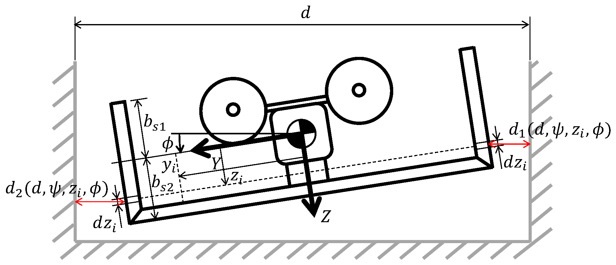
Given that the Aerotrain runs in a U-shaped guideway, the aerodynamic force generated from the guide wings are also under the WIG effect. The aerodynamic force
along
Y-axis is the combination of the aerodynamic force from 4 guide wings
.
Using the same idea as the aerodynamic force in the
Z-axis, where the distance
plays the role of the height
and
plays the role of the spanwise
, the coefficient of differential force of the guide wing at the spanwise
, as shown in the
Figure 8 and
Figure 9, could be written as follows [
21]:
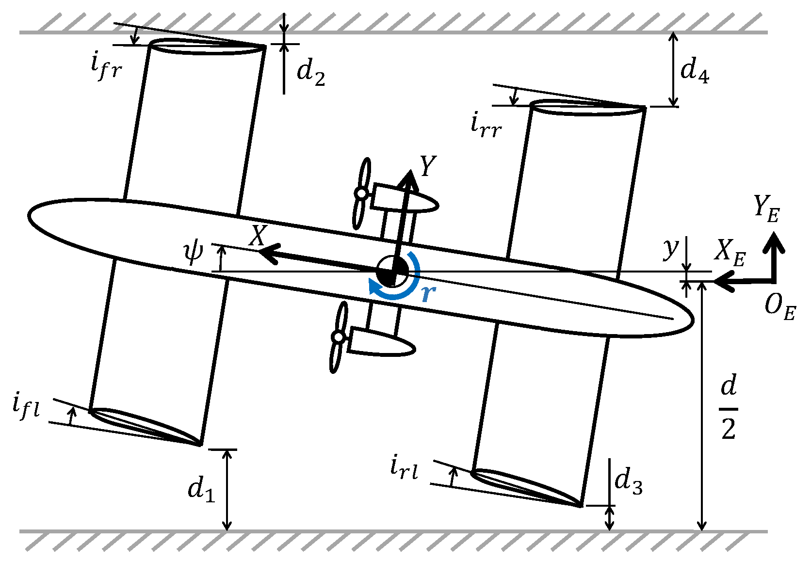
where
is the yawing angle;
are the mounting angle of the front left, front right, rear left, rear right guide wing relatively;
r is the yawing angular velocity;
d is the width of the guideway;
is the sideslip angle;
are the angle of attack of the guide wings.
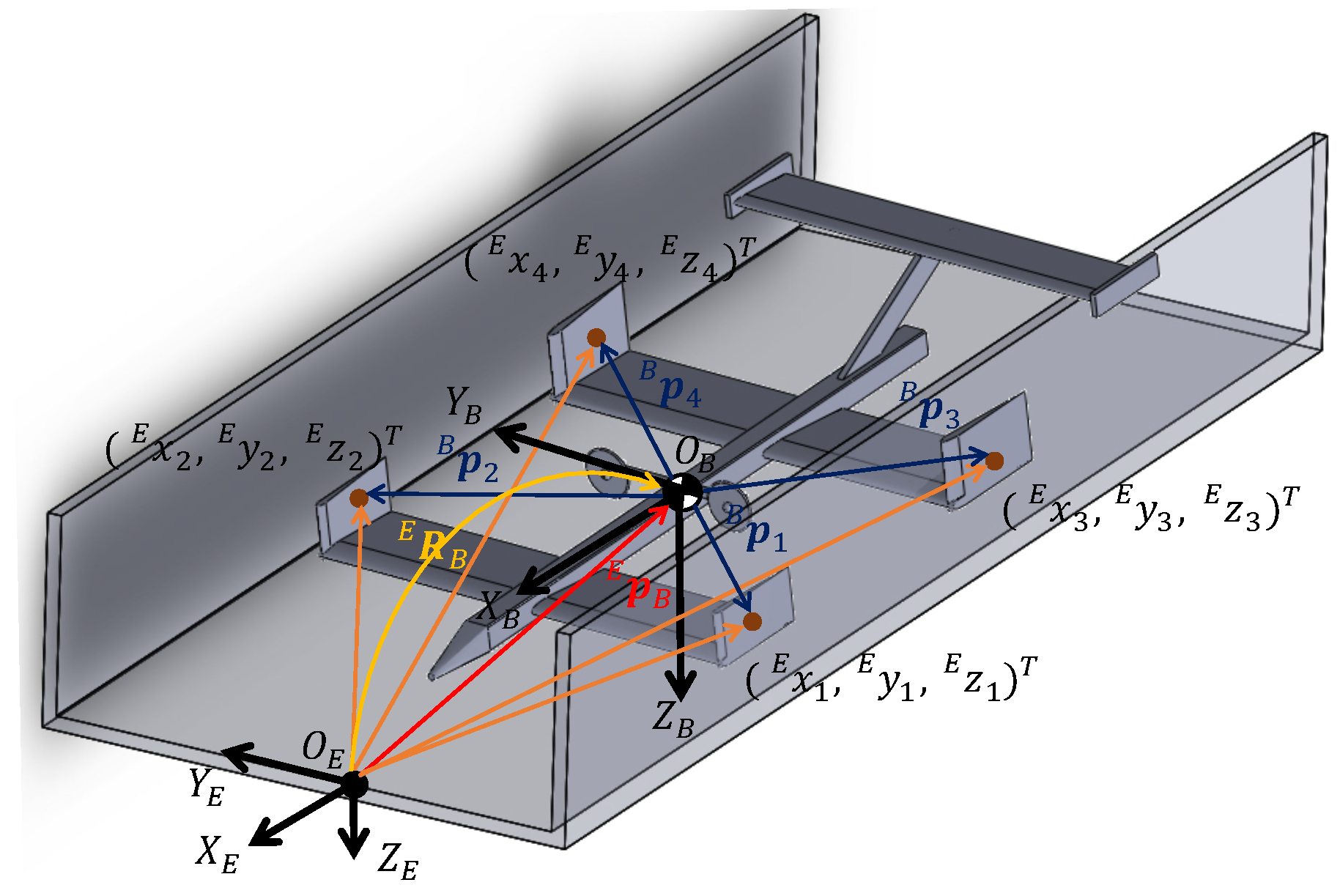
The distance
from the trailing edge of the guide wing to the wall could be calculated with respect to the inertial system
as shown in
Figure 10. The position vector of a point on the guide wing in the inertial system
could be obtained from the position vector in the body-fixed system
by the homogeneous translation matrix
as follows:
where
is the rotation matrix and
is the position vector of the origin of the body-fixed system with respect to the inertial system.
In the body-fixed system, for example, the position vector of a point on the front-left guide wing at the span wise
could be written as follows:
while in the inertial system, that position vector could be written as:
Using the Equations (
27)–(
30), the distance
could be calculated.
Therefore, by integrating along the wing span as shown in
Figure 8, the aerodynamic force along the
Y-axis of 4 guide wings could be expressed as follows:
where
are the chord length of the front and rear guide wings.
2.4. Aerodynamic Moment about the Axes
The aerodynamic moment about the
Y-axis (pitching moment)
is the sum of the moment of two levitation wings, the moment of the fuselage and the moment cause by the lift of these wings.
where
are the moments of the front and rear levitation wings, and it can be obtained by integrating along the wingspan as can be seen in
Figure 6.
The aerodynamic moment coefficient
about the
Y-axis at the spanwise
of two levitation wings are also under the WIG effect, therefore it can be computed from the Equations (
6)–(
8) as follows [
15]:
where
are the obtained constants from the experimental results [
20]. The constants are different between each levitation wing because of the generated downwash behind the front levitation wing.
The moment of the fuselage
is expressed as follows [
22]:
where
is the volume of the equivalent fuselage [
22] of the Aerotrain.
The moment about the
X-axis (rolling moment)
is obtained from the aerodynamic lift from the main levitation wings
, the front guide wings
, the rear guide wing
[
21], and the roll damping moment caused by yaw rate of the front levitation wing
and rear levitation wings
.
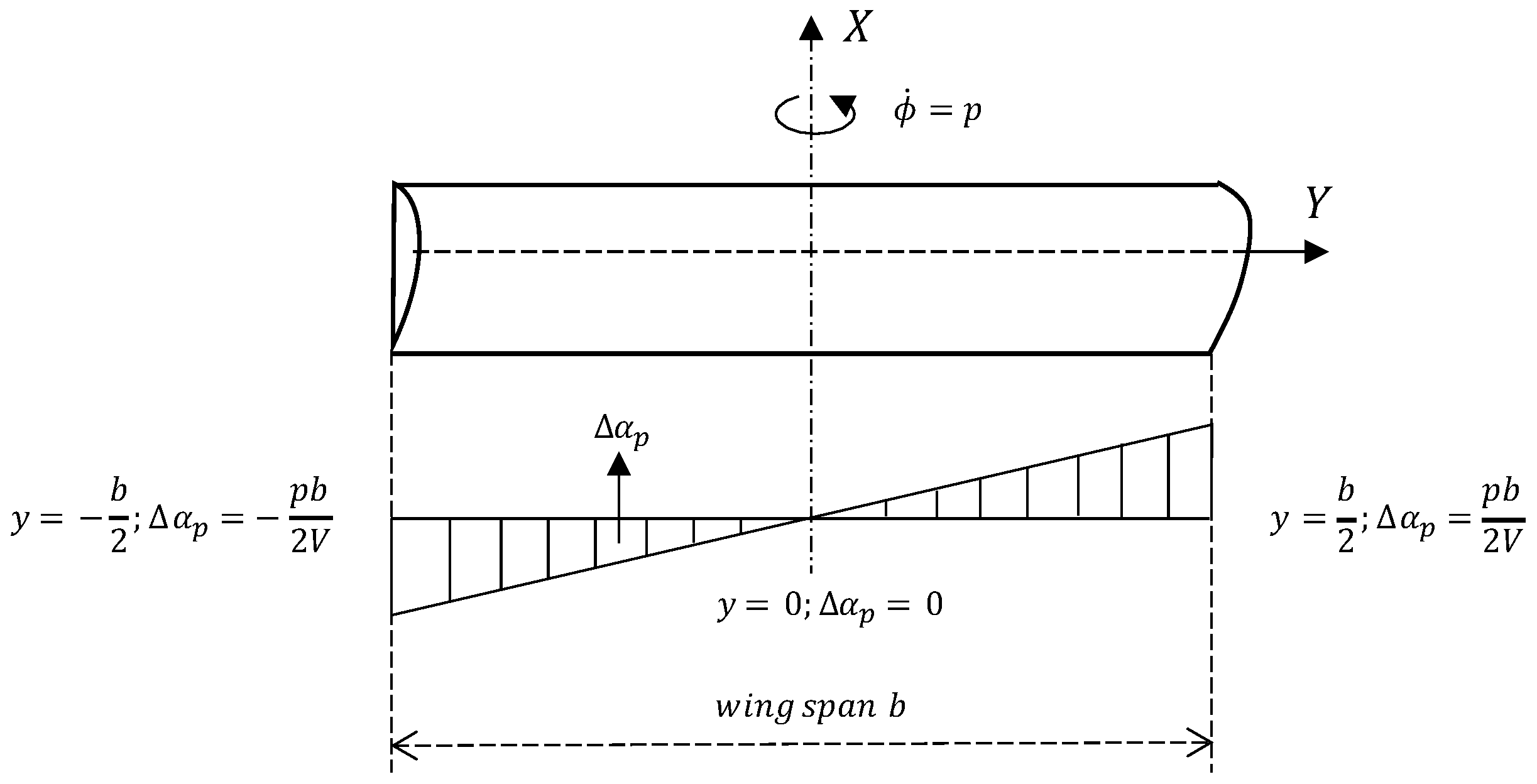
In rolling motion, the aerodynamic lift of the main levitation wings has the derivation from roll rate
. As can be seen in the
Figure 11, the positive roll rate induces a positive angle of attack at the right-wing tip of
. Because of roll rate is occurring about the
X-axis, the induced angle of attack varies linearly from
at the right wing tip to
at the left wing tip [
23]. Therefore, the angle of attack of the front levitation wing and rear levitation wing in lift coefficient
could be written as:
The roll damping moment caused by yaw rate is defined by [
23]:
where
is the dynamic pressure,
is the moment of inertial in
X-axis,
V is the airspeed,
is the yaw rate derivative in the roll damping moment.
Without the vertical tail, as an initial approximation, based on elementary wing strip theory approach, the yaw rate derivative in the roll damping moment
could be written as [
23]:
Therefore, the rolling damping moment caused by the yaw rate of the front and rear levitation wings could be written as:
The aerodynamic moment about the
Z-axis (yawing moment)
is the total moment of the guide wings, the moment of the side force from the guide wings and the moment of the fuselage:
where
are the moments of guide wings under WIG effect and could be computed in the same way as the moment of the levitation wings by integrating along the wingspan;
is the moment of the fuselage.
As was mentioned in the introduction, the guide wings is also under WIG effect. Therefore, the aerodynamic moment coefficients
of the guide wings at the wingspan
can be computed from the Equations (
6)–(
8) as follows:
where
are obtained constants from the experimental results [
20]. The guide wings at the front and rear levitation wings have different constants because of the downwash occurs when the airflow passes the front guide wings.
The moment of the fuselage
is expressed as follows [
22]:
where
is the volume of the equivalent fuselage [
22] of the Aerotrain.
2.5. Horizontal Tail Model
The lift coefficient and moment coefficient of the horizontal tail is a function of the angle of attack and the angular velocity [
19]. Depending on the angle of attack
, the lift coefficient
is directly related to the mounting angle
and the downwash angle
caused by the air flowing through the main wing.
In the case of the Aerotrain, the horizontal tail is located at the rear side of the train and at a high location so that the downwash flow does not affect the tail. Thus, the downwash angle is zero,
. Another assumption is that the horizontal tail has symmetry airfoil and does not generate any aerodynamic force when the angle of attack is zero, which means that the chord line is parallel to the
X-axis in the body-fixed system or the mounting angle
. As for the thin, symmetric airfoil [
24], the lift coefficient could be written as follows:
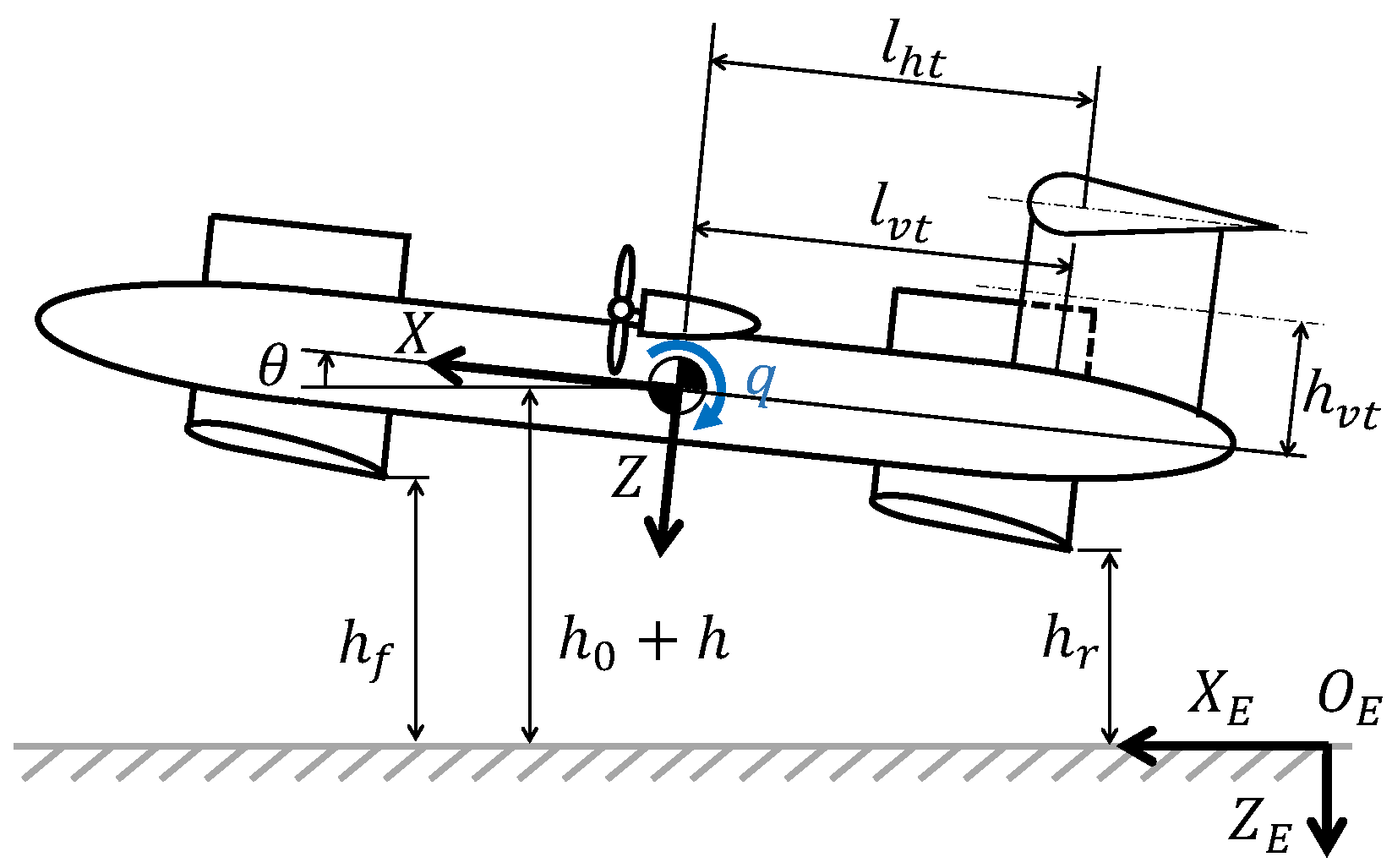
The horizontal tail is located at a distance
from the origin of the body-fixed coordinate system to the aerodynamic center of the tail as shown in
Figure 12. Thus, the effect of pitching rate
q in terms of the changing of angle of attack
is described as:
Thus, the lift coefficient of the horizontal tail caused by the pitching rate is:
Therefore, the total lift force coefficient is the sum of these two coefficients:
The total pitching moment from the horizontal tail is also a function of the angle of attack
and the pitching rate
q and it could be written as:
2.6. Vertical Tail Model
Similar to the horizontal tail model, we assume that the vertical tail has a symmetry airfoil, locates at a distance
from the CoG of the Aerotrain to the aerodynamic center of the tail as shown in
Figure 12, and the chord line is align to the
X-axis in the body-fixed system. Thus, the side force coefficient of the vertical tail
caused by the angle of attack
and the yaw rate
r is described as:
The side force of the vertical tail also contributes a rolling moment:
where
is the distance from the
X-axis of the body-fixed system to the
vertical tail wingspan as shown in
Figure 12,
is the vertical tail area.
The total yawing moment from the vertical tail is also the function of the angle of attach
and the yawing rate
r and it could be written as:
2.7. Dihedral Levitation Wing Model
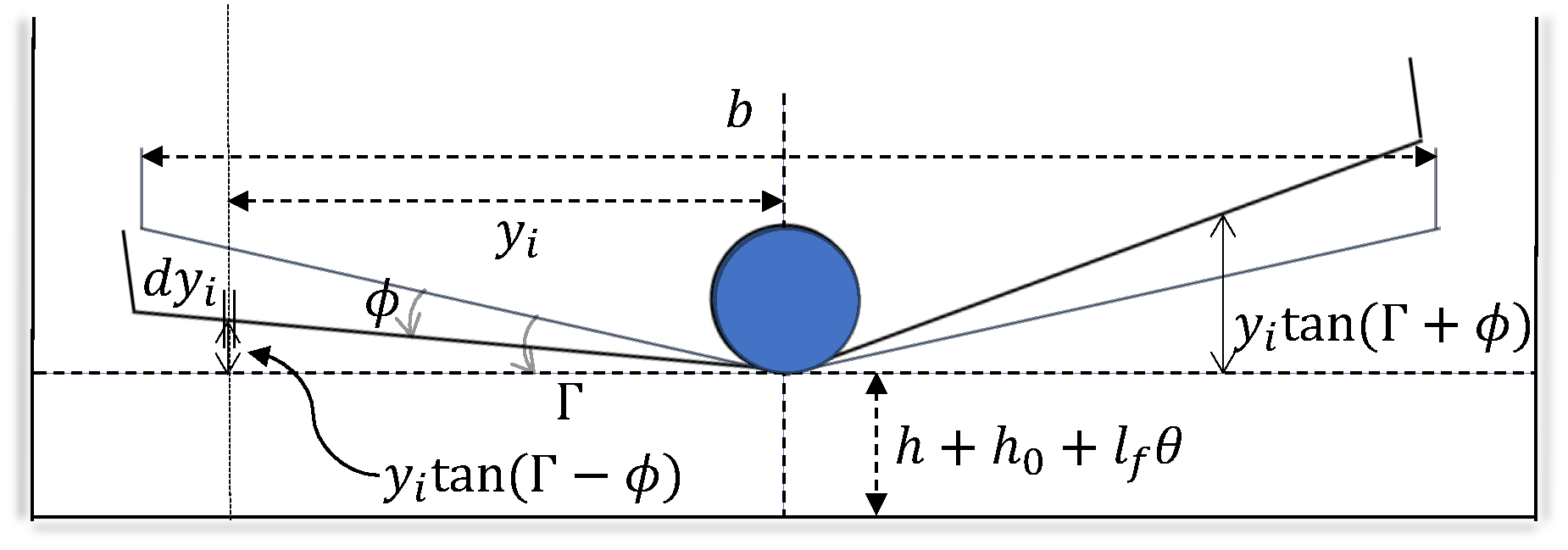
The dihedral wing design is easily found in the commercial and training aircraft because of its efficient rolling damping, that is important to keep the aircraft stable. When a rolling motion happens, it also generate a coupled yawing motion, and results a side slip angle
. Assumed that the dihedral angle
is small enough, the differential angle of attack
[
23] on the left and right panel of the levitation wing change in opposite way.
Thus, the difference amount of lift on the left and the right panel of the levitation wing generates a recovering moment. In dihedral design of the front wing, the angle of attack of the front left levitation wing
and front right levitation wing
in the Equation (
13) could be written as:
Figure 13 shows the height of the front left wing
and front right wing
in dihedral wing design. The height of the front wing in the Equation (
11) could be written as:
3. Simulation and Discussion
To evaluate the dynamic stability of the Aerotrain, a three-dimensional dynamic model has been developed in the MapleSim [
25] environment using a rigid body model as shown in
Figure 14. The advantage of the MapleSim over the others is its friendly user interface and its sufficiency when creating custom components that are not available in the default library. Moreover, by improving the detail of each component (for example, the roll rate and yaw rate derivatives in the rolling moment), the accuracy of the previous model proposed in Reference [
21] could be enhanced with unnoticed additional computational cost.
Base on the mathematical equations, the aerodynamic components, such as lift and moment of the levitation wings and the guide wings has been created as the customer components. The total net force in the Z-axis which includes the lift from the levitation wing, the horizontal tail and the total net force in Y-axis includes the side force from the guide wings and the vertical tail were applied to the Aerotrain body through the “Apply World Force” component. Similar to the force, the total net moment about axes was also applied to the body of the train through the “Apply World Moment” component.
As a case study, the parameters used in the simulation in
Table 1 were approximate from the experimental ARTE02 prototype developed in Reference [
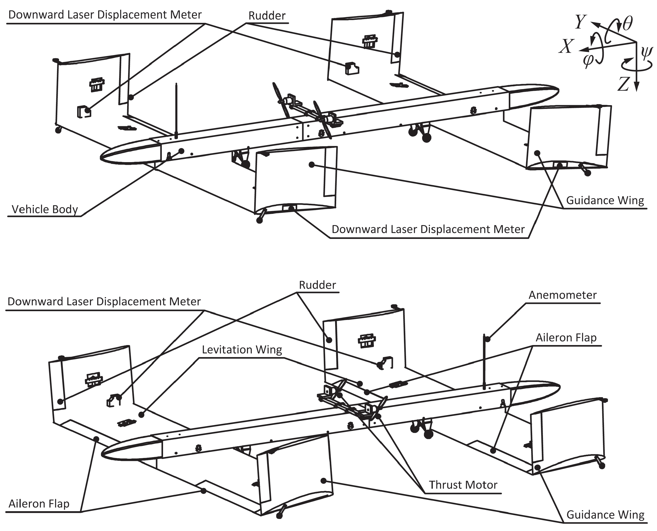
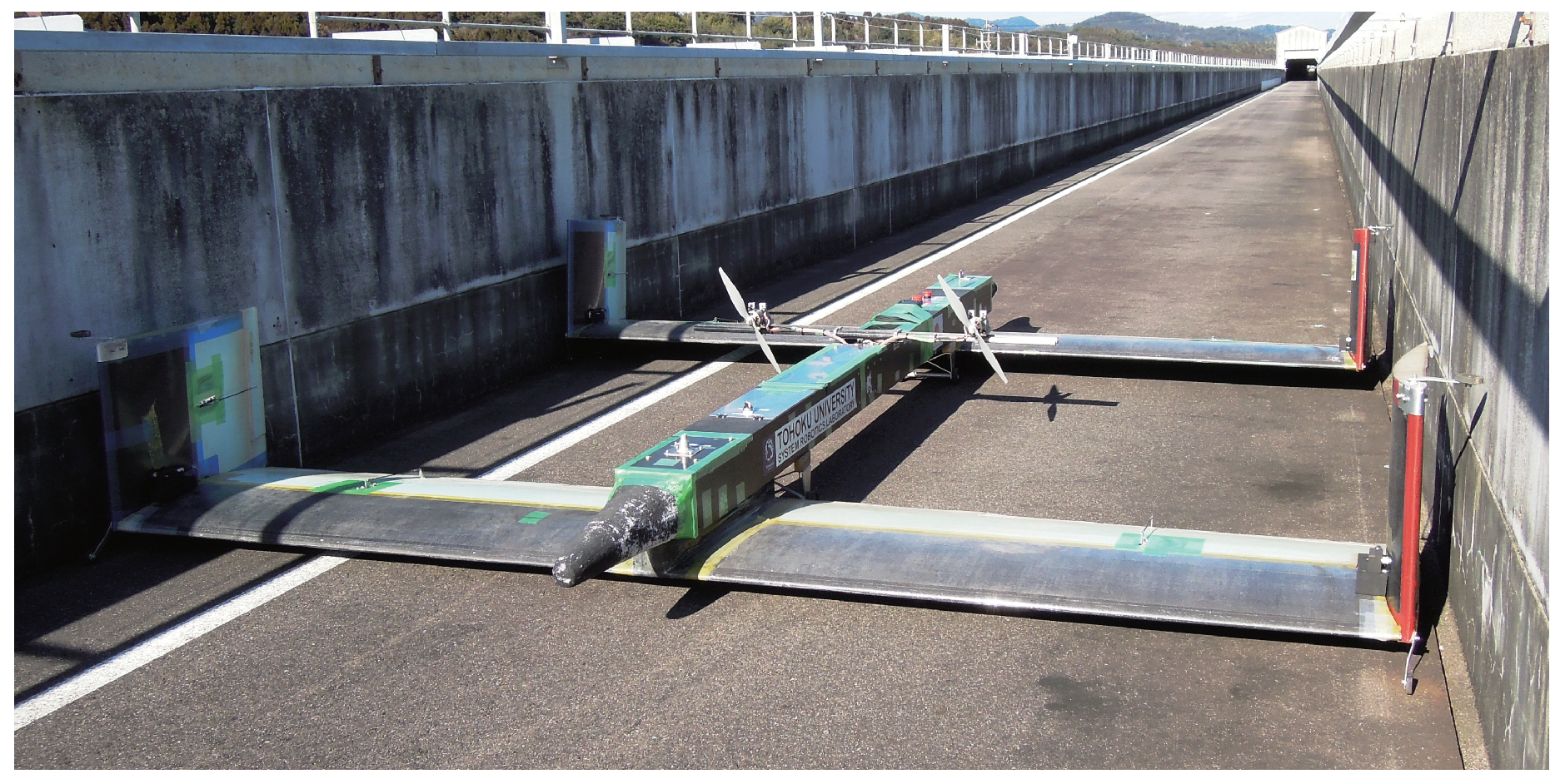
16]. The mass of the prototype was measured while the other parameters are designed values. The prototype, as shown in
Figure 15,
Figure 16 and
Figure 17, is equipped with four aileron flaps which control the pitching and rolling motion, and four rudders which control the yawing motion according to the distance between the vehicle body and the guideway which is measured from the laser displacement sensors. By using physical parameters of ARTE02 prototype, the evaluation of the state space equation of the dynamic model of Aerotrain was shown that the system is unstable but controllable [
16].
At the equilibrium state, according to each design of the Aerotrain, the velocity is computed, so that the generated aerodynamic lift is equal to the vehicle’s weight; by moving the CoG of Aerotrain along X-axis of the body-fixed coordinate system, the distance of the front levitation wing and of the rear levitation wing are calculated, so that the total moment applies to the model is zero. In order to evaluate the dynamic stability of the Aerotrain, during 25 s of the simulation time, the external disturbances were applied to the body after 2 s to observe the responsibility of the model. The external disturbances include a force of 50 N which applied in Z axis, two moments of 10 which applied to rotate the body about the X-axis and Z-axis.
3.1. Longitudinal Dynamic Stability
With the design of the experimental prototype ARTE02, at the equilibrium state, it requires a velocity of
m/s, and the CoG of the vehicle is located at a location such that
m,
m. A horizontal tail with the area of
m
, located at
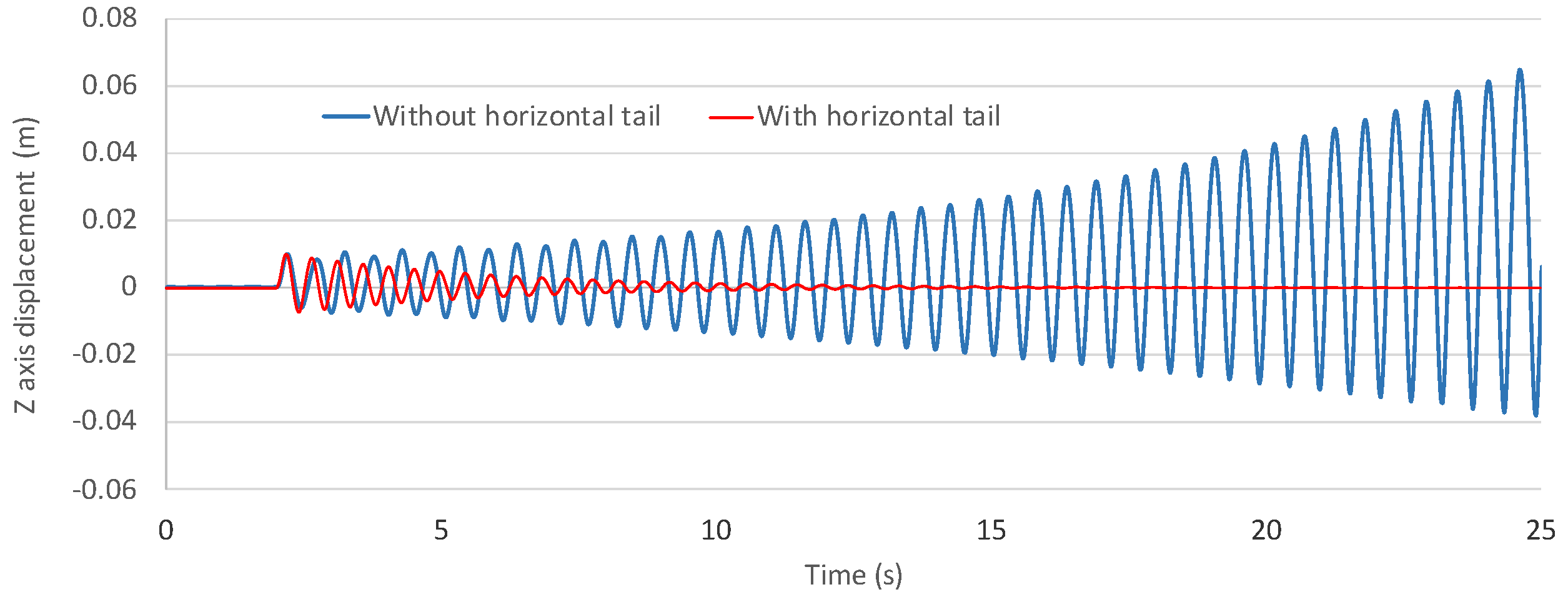
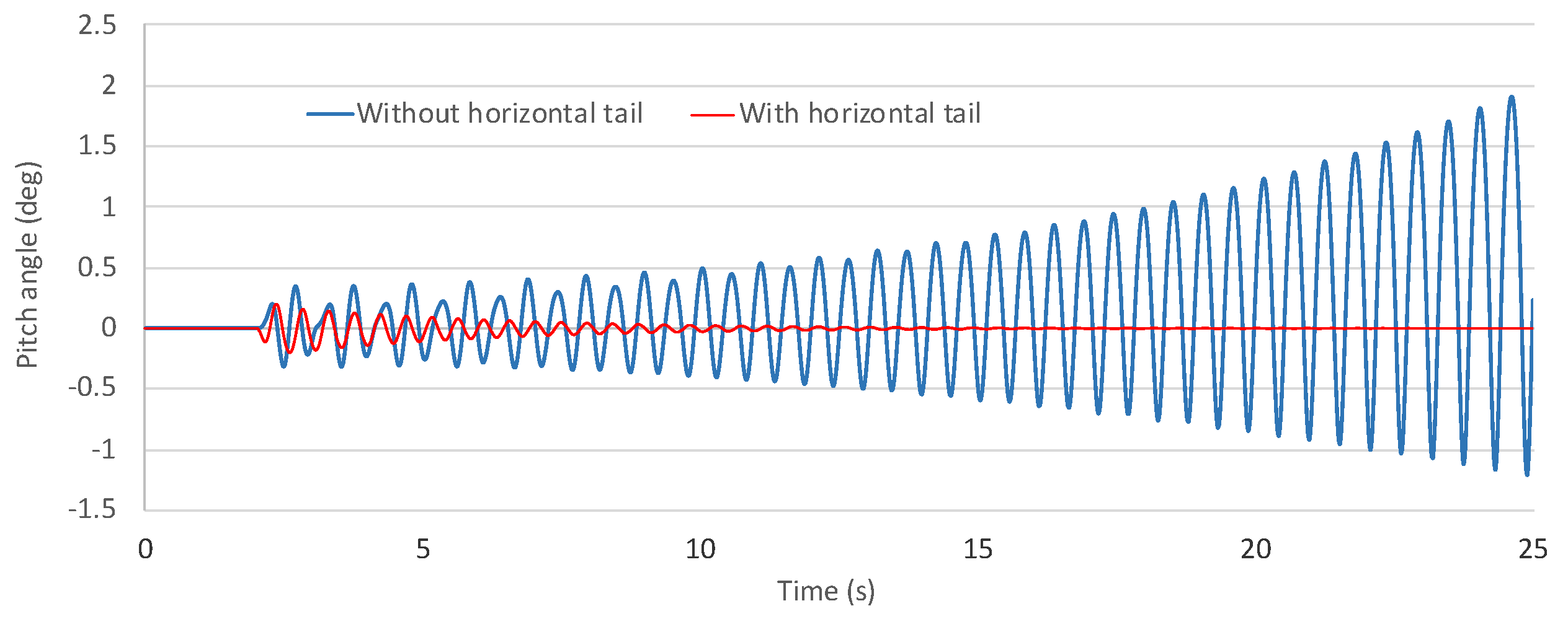
m was added to the model. At the same condition, with the horizontal tail, the displacement in the
Z-axis and pitch angle
have been convergent as shown in
Figure 18 and
Figure 19 thanks to the spring element
and damper element
q. The simulation results have clearly proved that the effectiveness of the horizontal tail still remained in the three-dimensional model.
In Wang’s study [
26], it was found that the configuration with a higher horizontal tail has insignificant effects on the aerodynamic efficiency of a WIG craft. Thus, based on the above confirmation, the design of the horizontal tail (area
and location
) is targeted to investigate the relationship between the design and the longitudinal dynamic stability of the Aerotrain. First, the horizontal tail area is fixed as 0.5 m
, the distance from the CoG of the Aerotrain to the aerodynamic center of the horizontal tail
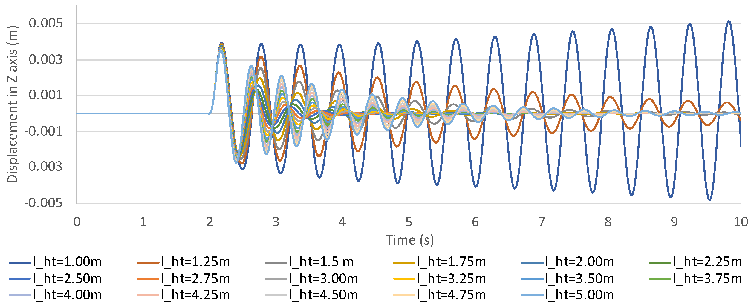
ranges from 1 m to 5 m at a 0.25 m step. As can be seen in
Figure 20, the response of the Aerotrain in
Z-axis is different at each location. Especially, at the location of 1 m the displacement in the
Z-axis becomes divergent, which means the design does not have longitudinal dynamic stability.
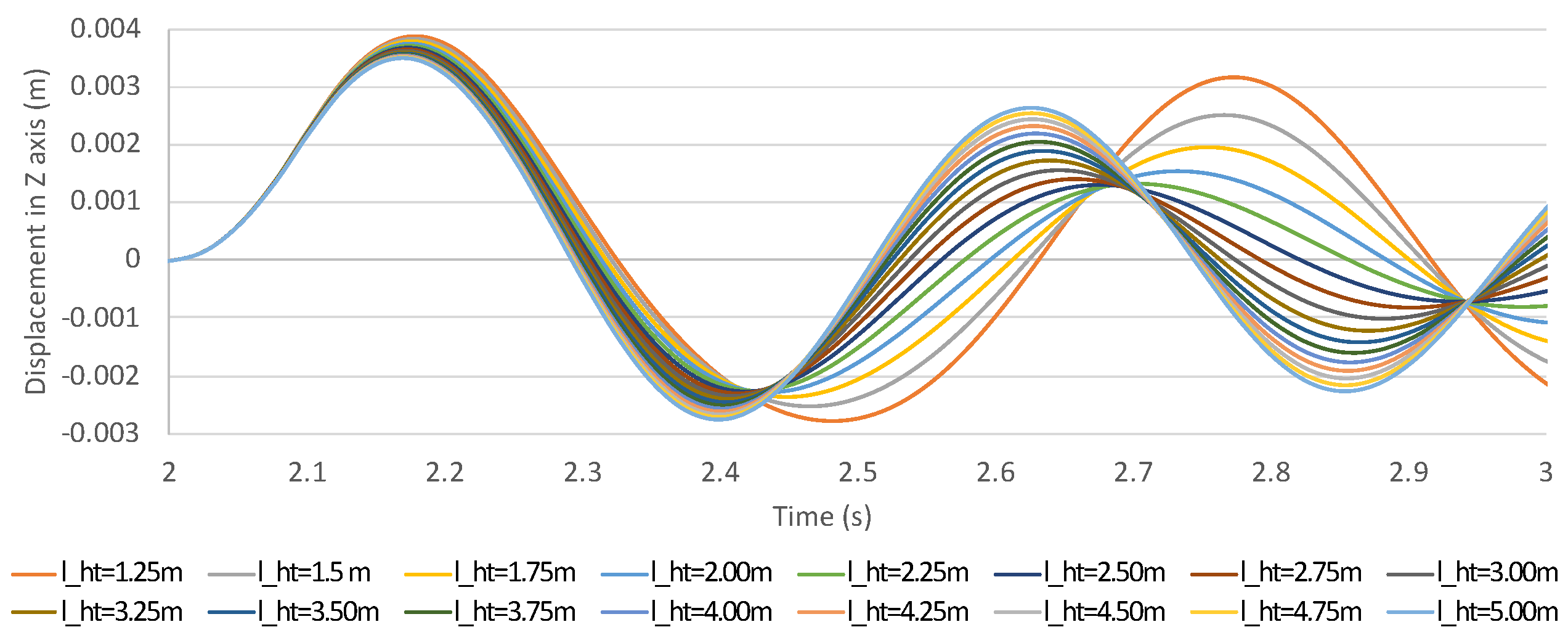
Zooming in the detail of the
Figure 20 at the range from 2 s to 3 s,
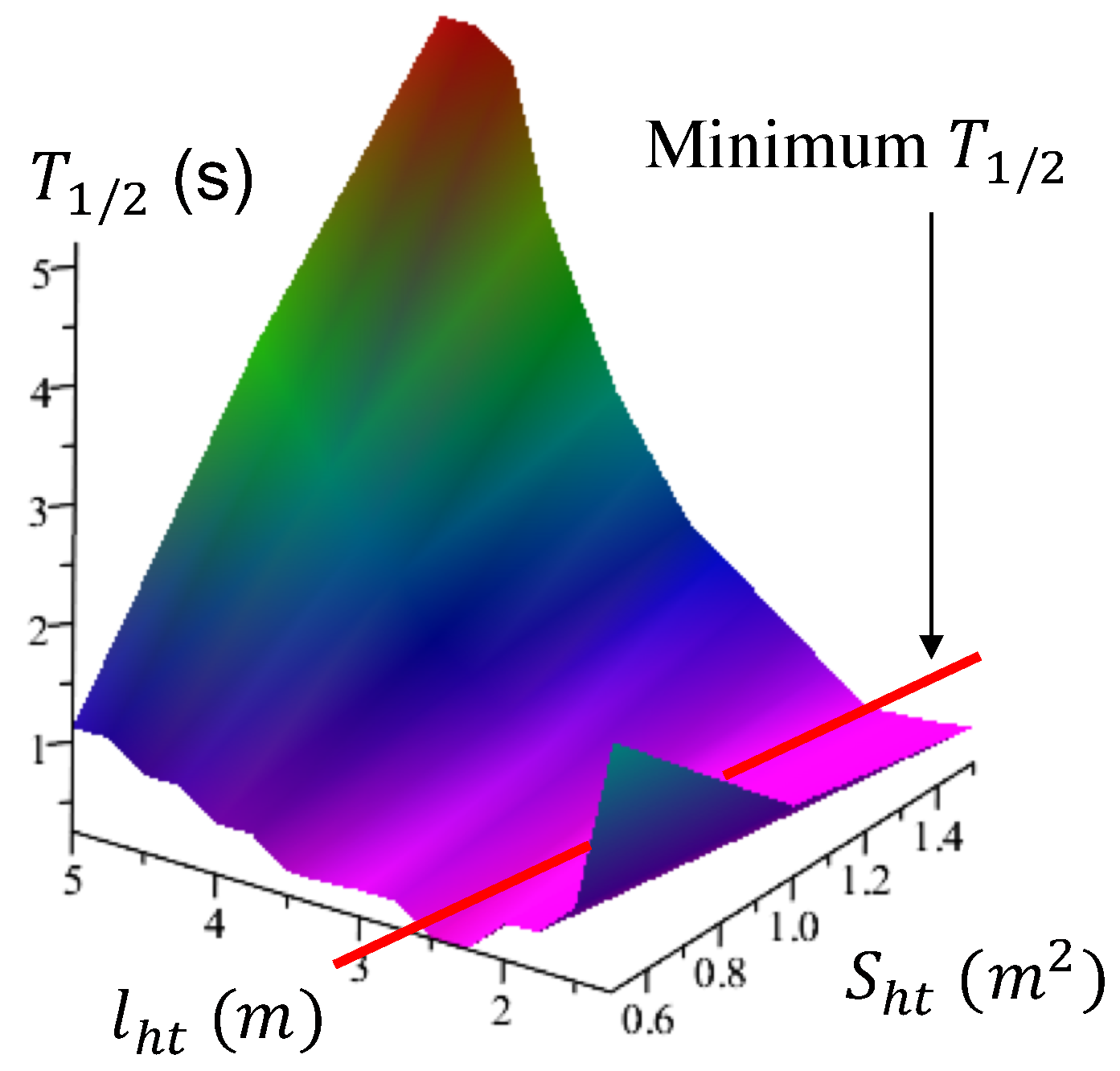
Figure 21 shows that after one period, the location of 2.25 m and 2.5 m have the highest amplitude reduction, therefore have the best performance in terms of dynamic stability. In order to investigate the relationship between the location
, the area
and the longitudinal dynamic stability,
has been introduced.
is the time to damp to half amplitude from maximum amplitude, so that smaller
, better dynamic stability.
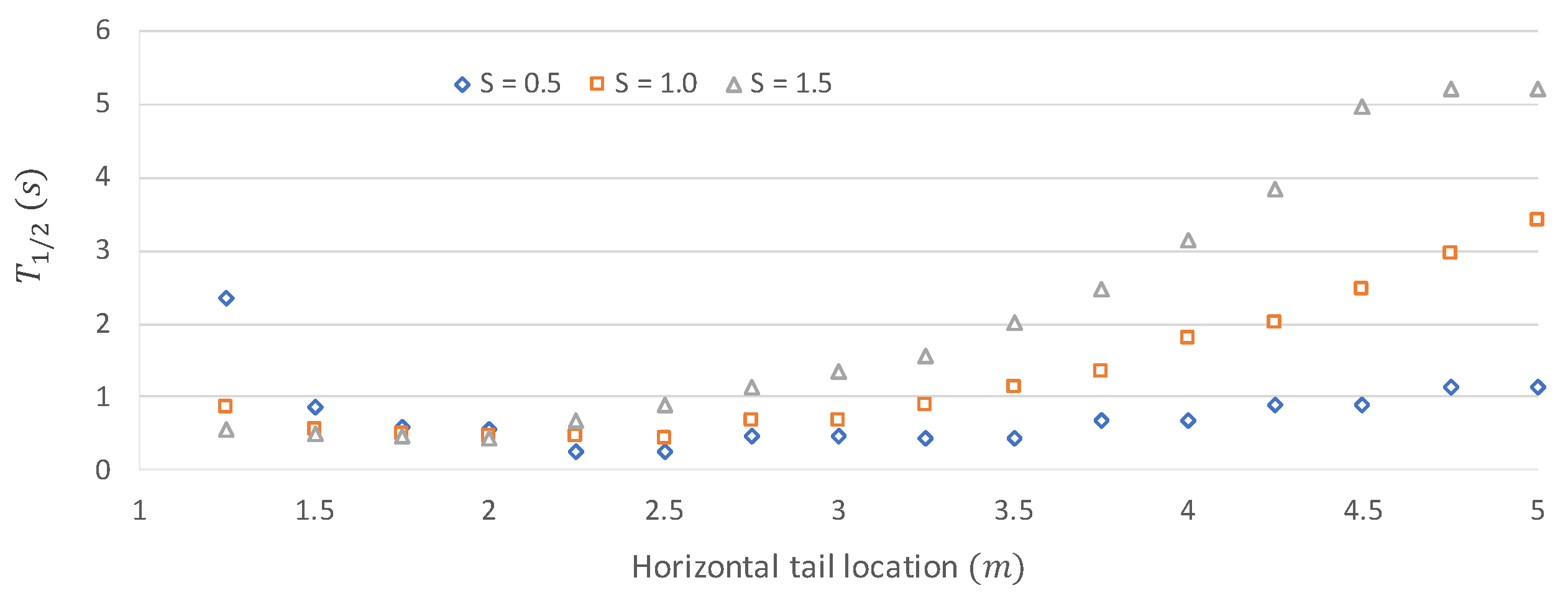
At the same range of the horizontal tail location, two more different horizontal tail area of 1 m
and 1.5 m
have been simulated. The relationship between the horizontal tail location, area and the dynamic stability represented by
has been clarified in
Figure 22 and
Figure 23. As a simple prediction, the ideal design of the horizontal tail could be described in a straight line form:
3.2. Lateral Dynamic Stability
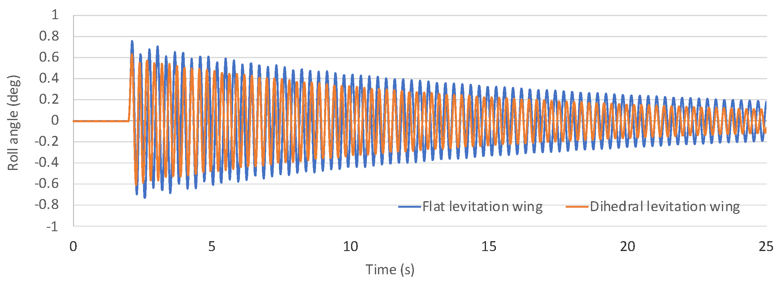
The response of the Aerotrain to the rolling disturbance of 10
is showed in the
Figure 24. The simulation result shows that the roll angle
has been convergent, or the design of flat levitation wing of Aerotrain can maintain lateral dynamic stability. The result again confirms the advantage of WIG effect in lateral stability of WIG effect vehicles, that was found through the numerical studies by Amir [
27]. However, the damping is insufficient to damp the vibration in a short time. As a simple comparison, the front levitation wing has been replaced by a dihedral wing with
degrees while maintaining the same wingspan in order to fit into the guideway. The dihedral wing design caused a reduction of the aerodynamic lift at the front levitation wing. Thus, it requires a velocity of 42.8 km/h (increased 23.5% in comparison with the flat levitation wing design) to compensate that reduction. Also, the reduction of the aerodynamic lift at the front levitation wing shifted the CoG of the vehicle rearward, so that
m,
m to maintain the equilibrium state.
In the dihedral levitation wing design, the vibration amplitude is smaller than that of the flat levitation wing design, but the trend is the same. Simulation result shows that the dihedral levitation wing design can increase the stability as it does on the airplane. However, to trade off with that small increasing of the stability, with the same wing span, the dihedral levitation wing requires a higher velocity to compensate the reduction of the aerodynamic lift at the front levitation wing. Therefore, it can be said that the dihedral levitation wing design is not suitable for the Aerotrain application. The lateral stability of the Aerotrain still needs the assist of the control system, especially for the damping.
3.3. Directional Dynamic Stability
By keeping a horizontal tail with the area of
m
, located at
m, a vertical tail with the area of
m
, located at
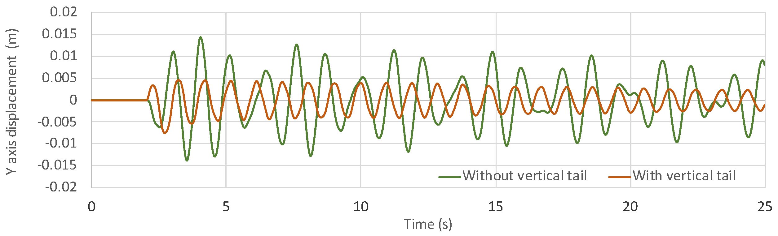
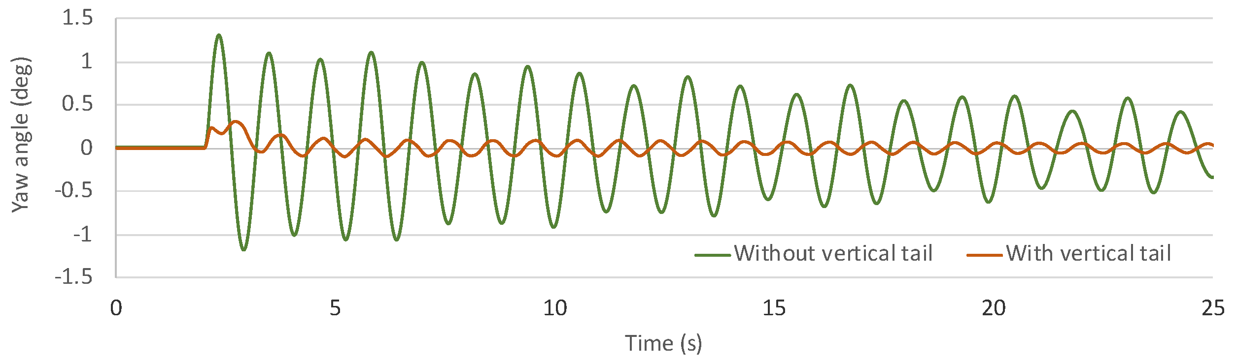
m, was added to the model. As can be seen in
Figure 25 and
Figure 26, the design without the vertical tail can achieve the directional stability. However, the directional damping is insufficient. At the same condition, with the vertical tail, the displacement in the
Y-axis and yaw angle has significantly reduction of the vibration amplitude.
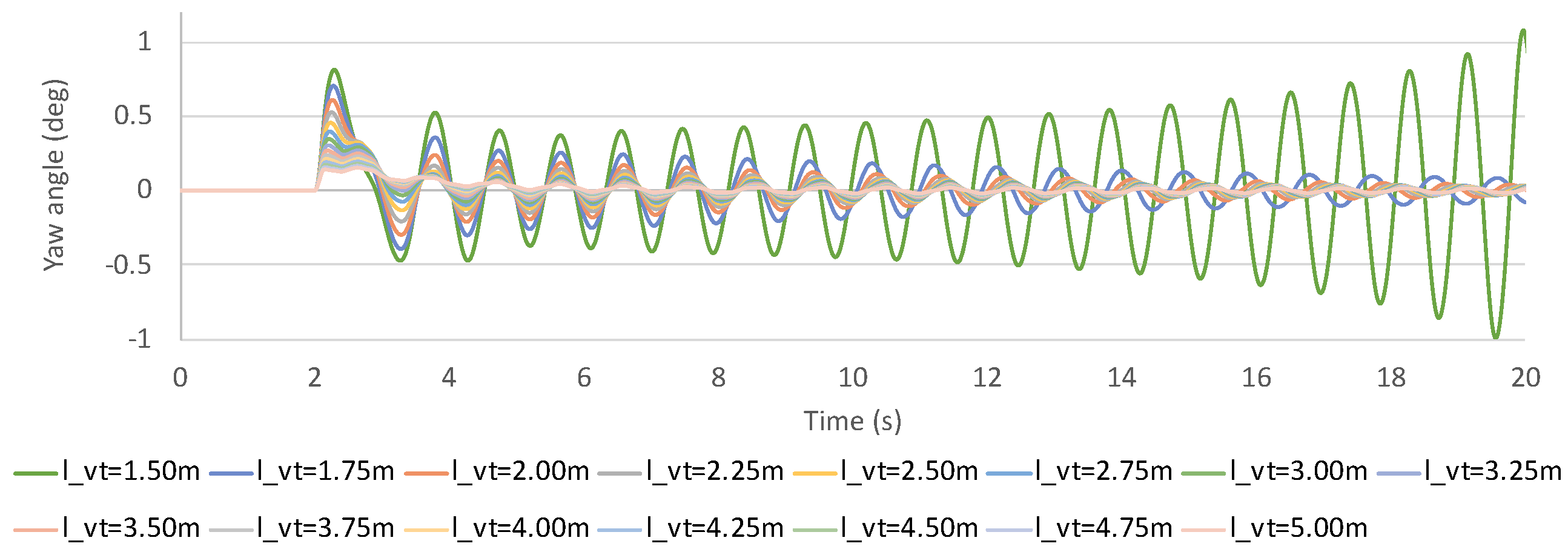
In order to investigate the vertical tail design (vertical tail location
and area
) and the directional dynamic stability, various designs has been simulated. First, at a fixed area of
m
, the location of the vertical tail ranges from 1.5 m to 5 m at 0.25 m step. The simulation results have been shown in
Figure 27. Since the displacement in the
Y-axis and the yaw angle show the same trend of the vibration amplitude reduction, we can use one of them to evaluate the effect of the vertical tail. In this paper, the yaw angle was used. At different location, the maximum amplitude of the Yaw angle change accordingly. Therefore, the maximum amplitude
is used to evaluate the design of the vertical tail instead of
, that was used in case of the horizontal tail. It could be said that the smaller
, the better directional stability.
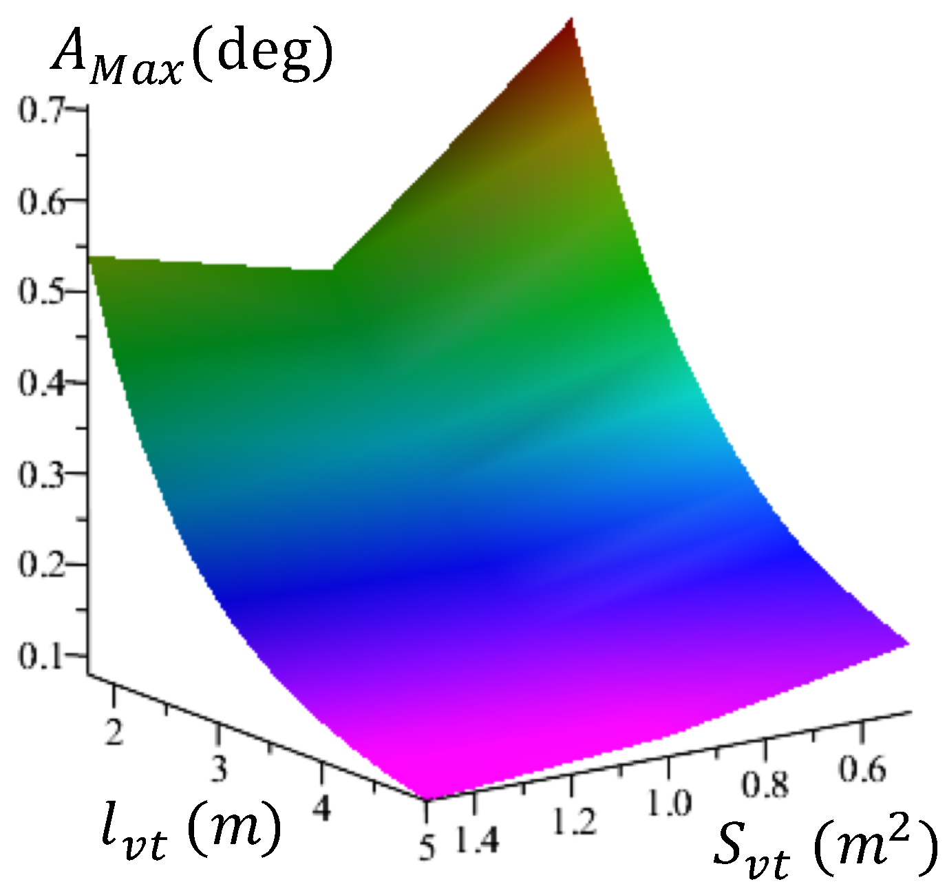
At the same range of the vertical tail location, two more different vertical tail area of
m
and
m
have been simulated. The relationship between the vertical tail location
, area
and the directional dynamic stability represented by
has been clarified in
Figure 28 and
Figure 29. The larger vertical tail area, the better directional stability and (or) the farther vertical tail location, the better stability.
4. Conclusions and Future Work
In this paper, the three-dimensional dynamic model of the Aerotrain has been developed taking into account the nonlinear aerodynamic forces and moments under the WIG effect. Compared with the previous studies [
19,
21] the side force from the 4 guide wings, the aerodynamic lift and moment from the levitation wings, the horizontal tail and the vertical tail have been integrated into the rigid body model to make the dynamic model more specific so that it will be useful for the optimization studies.
Based on this dynamic model, the design-stability relation of the Aerotrain has been investigated. The horizontal tail with several designs in tail location and tail area has been simulated to evaluate the longitudinal dynamic stability. The dihedral levitation wing design has been considered to evaluate the lateral dynamic stability. As for the directional dynamic stability, several designs of the vertical tail in tail location and tail area has been considered as well.
The area and location of the horizontal tail have a great effect on the longitudinal stability. The horizontal tail shows its best performance if the tail area is a function of the tail location. The dihedral levitation wing, expected to improve the longitudinal stability, did not show significant change. The vertical tail showed its effectiveness in terms of directional stability as the maximum vibration was significantly reduced. The position and location of the vertical tail also have a great effect on the directional stability. Unlike the horizontal tail, the larger vertical tail area, the better directional stability and (or) the farther vertical tail location, the better stability. Therefore, the design of the vertical tail is depended on the application purpose.
In the future, based on this dynamic model, the force in X-axis will be considered to complete the 6-degrees of freedom of the three-dimensional model, and the contribution of each effect on the model accuracy will be taken into account. The sensitivity analysis will be carried out by changing one parameter at a time and keeping all other parameters fixed to figure out what would be the consequences of parameters estimation bias to the model simulation accuracy. Figuring out which parameter is more sensitive than the others about the stability will benefit not only the initial design phase of Aerotrain but also the safety of the vehicle. Then, the next studies will be focused on the experiment of a small-scale prototype in order to evaluate the reliability of the dynamic model. The experimental results will be useful to develop a full-scale prototype and the dynamic model of a multi-cars design as well.
Author Contributions
Conceptualization, Q.H.L., J.J. and Y.S.; methodology, Q.H.L., J.J. and Y.S.; software, Q.H.L. and J.J.; writing—original draft preparation, Q.H.L.; writing—review and editing, Q.H.L., Y.S., D.M. and Y.T.; supervision, Y.S. and Y.T. All authors have read and agreed to the published version of the manuscript.
Funding
This work was partially supported by JSPS KAKENHI 26420814.
Conflicts of Interest
The authors declare no conflict of interest.
References
- Sugahara, Y.; Kikuchi, S.; Kosuge, K.; Kohama, Y.P. Levitation Control of AEROTRAIN: The Design and System of Experimental Manned Wing-in-Ground Vehicle ART003R. J. Robot. Mechatron. 2013, 25, 1097–1104. [Google Scholar]
- Omio Homepage. Available online: https://www.omio.co.uk/trains/high-speed (accessed on 13 March 2019).
- Lai, C.; Ren, B.; Zhou, Y. Influence of wing angle of attack and relative position on the aerodynamics of aerotrain. Adv. Mech. Eng. 2017, 9. [Google Scholar] [CrossRef]
- Kohama, Y. An application of ACV to railway transportation. In Proceedings of the 25th Aircraft Symposium, Columbus, OH, USA, 22–25 April 1987; pp. 128–131. (In Japanese). [Google Scholar]
- International High-speed Rail Association Homepage. Available online: https://www.ihra-hsr.org (accessed on 13 March 2019).
- Rozhdestvensky, K.V. Aerodynamics of a Lifting System in Extreme Ground Effect; Springer Science & Business Media: Berlin/Heidelberg, Germany, 2000. [Google Scholar]
- Kohama, Y. Mechanical civilization induced earth pollution problem, and aero-train. Trans. Jpn. Soc. Mech. Eng. Ser. B 2005, 71, 1–5. (In Japanese) [Google Scholar]
- Hameed, H. The design of a four-seat reverse delta WIG craft. Maldives Natl. J. Res. 2019, 7, 7–28. [Google Scholar]
- Matdaud, Z.; Zhahir, A.; Pua’at, A.A.; Hassan, A.; Ahmad, M. Stabilizing Attitude Control for Mobility of Wing In Ground (WIG) Craft—A Review. In Proceedings of the IOP Conference Series: Materials Science and Engineering, Bangkok, Thailand, 17–19 May 2019; Volume 642, p. 012005. [Google Scholar]
- Matjasic, K. WIG (Wing In Ground effect) craft in military and paramilitary applications. In Proceedings of the NATO Conference, TO-AVT Symposium, Brussels, Belgium, 7–11 April 2003. [Google Scholar]
- de Divitiis, N. Performance and stability of a winged vehicle in ground effect. J. Aircr. 2005, 42, 148–157. [Google Scholar]
- Rozhdestvensky, K.V. Wing-in-ground effect vehicles. Prog. Aerosp. Sci. 2006, 42, 211–283. [Google Scholar]
- Wigetworks Homepage, Airfish 8. Available online: https://www.wigetworks.com/airfish-8 (accessed on 2 November 2020).
- Kikuchi, S.; Ohta, F.; Kato, T.; Ishikawa, T.; Kohama, Y. Development of a stability control method for the aero-train. J. Fluid Sci. Technol. 2007, 2, 226–237. [Google Scholar]
- Sugahara, Y.; Ikeuchi, Y.; Suzuki, R.; Hirata, Y.; Kosuge, K.; Noguchi, Y.; Kikuchi, S.; Kohama, Y.P. Levitation control of experimental wing-in-ground effect vehicle along Z axis and about roll and pitch axes. In Proceedings of the 2011 IEEE International Conference on Robotics and Automation, Shanghai, China, 9–13 May 2011; pp. 8–13. [Google Scholar]
- Sugahara, Y.; Minagawa, N.; Kosuge, K.; Kohama, Y.P. Levitation control of experimental wing-in-ground effect vehicle along Y and Z axes and about three axes. In Proceedings of the 2012 IEEE/RSJ International Conference on Intelligent Robots and Systems, Algarve, Portugal, 7–12 October 2012; pp. 488–494. [Google Scholar]
- Matsumoto, T.; Sugahara, Y.; Kikuchi, S.; Honda, Y.; Kohama, Y. Study on the vehicle body design and stability of Aero-Train–1st report: Longitudinal dynamic model. In Proceedings of the 16th SICE System Integration Division Conference, Nagoya, Japan, 14–16 December 2015; pp. 1416–1419. (In Japanese). [Google Scholar]
- Raymer, D.P. Aircraft Design: A Conceptual Approach; American Institute of Aeronautics and Astronautics: Washington, DC, USA, 1992. [Google Scholar]
- Jong, J.; Matsumoto, T.; Honda, Y.; Sugahara, Y.; Kikuchi, S.; Kohama, Y. Study on the body frame design and stability of aero-train–2nd report: Effect of the horizontal tail on longitudinal dynamic model. In Proceedings of the 17th SICE System Integration Division Conference, Sapporo, Japan, 13–15 December 2016; pp. 549–553. (In Japanese). [Google Scholar]
- Honda, K. Longitudinal Stability of WIG with Tandem Configuration. Master’s Thesis, Tohoku University, Miyagi, Japan, 2002. (In Japanese). [Google Scholar]
- Jong, J.; Honda, Y.; Sugahara, Y.; Kikuchi, S.; Kohama, Y. Study on the body frame design and stability of aero-train–3rd report: Development of 3-dimensional dynamic model. In Proceedings of the JSME Conference on Robotics and Mechatronics, Koriyama, Japan, 19 June 2017. (In Japanese). [Google Scholar]
- Caughey, D.A. Introduction to Aircraft Stability and Control Course Notes for M&AE 5070; Sibley School of Mechanical & Aerospace Engineering Cornell University: Ithaca, NY, USA, 2011. [Google Scholar]
- Schmidt, L.V. Introduction to Aircraft Flight Dynamics; American Institute of Aeronautics and Astronautics: Reston, VA, USA, 1998. [Google Scholar]
- Anderson, J.D. Fundamental of Aerodynamics; McGraw-Hill: New York, NY, USA, 2011. [Google Scholar]
- Maplesoft Homepage. Available online: https://www.maplesoft.com/products/maplesim/ (accessed on 13 March 2019).
- Wang, H.; Teo, C.; Khoo, B.; Goh, C. Computational aerodynamics and flight stability of wing-in-ground (WIG) craft. Procedia Eng. 2013, 67, 15–24. [Google Scholar]
- Amir, M.; Maimun, A.; Mat, S.; Saad, M. Computational analysis of aerodynamic characteristics for wing in ground effect craft in lateral stability. In Proceedings of the IOP Conference Series: Materials Science and Engineering, Bangalore, India, 14–16 July 2016; Volume 152, p. 012003. [Google Scholar]
| Publisher’s Note: MDPI stays neutral with regard to jurisdictional claims in published maps and institutional affiliations. |
© 2020 by the authors. Licensee MDPI, Basel, Switzerland. This article is an open access article distributed under the terms and conditions of the Creative Commons Attribution (CC BY) license (http://creativecommons.org/licenses/by/4.0/).


